Article

Stiffness Data of High-Modulus Asphalt Concretes for Road Pavements: Predictive Modeling by Machine-Learning

1
Polytechnic Department of Engineering and Architecture (DPIA), University of Udine, Via del Cotonificio 114, 33100 Udine, Italy
2
Faculty of Civil Engineering, Czech Technical University, Thákurova 7, 166 29 Prague, Czech Republic
3
Department of Civil Engineering, University Campus, Aristotle University of Thessaloniki, 54124 Thessaloniki, Greece
*
Author to whom correspondence should be addressed.
Coatings 2022, 12(1), 54; https://doi.org/10.3390/coatings12010054
Submission received: 16 December 2021 / Revised: 29 December 2021 / Accepted: 31 December 2021 / Published: 3 January 2022
(This article belongs to the Special Issue Road Pavements for Reduction of Climate and Safety Risks)

Abstract

:
This paper presents a study about a Machine Learning approach for modeling the stiffness of different high-modulus asphalt concretes (HMAC) prepared in the laboratory with harder paving grades or polymer-modified bitumen which were designed with or without reclaimed asphalt (RA) content. Notably, the mixtures considered in this study are not part of purposeful experimentation in support of modeling, but practical solutions developed in actual mix design processes. Since Machine Learning models require a careful definition of the network hyperparameters, a Bayesian optimization process was used to identify the neural topology, as well as the transfer function, optimal for the type of modeling needed. By employing different performance metrics, it was possible to compare the optimal models obtained by diversifying the type of inputs. Using variables related to the mix composition, namely bitumen content, air voids, maximum and average bulk density, along with a categorical variable that distinguishes the bitumen type and RAP percentages, successful predictions of the Stiffness have been obtained, with a determination coefficient (R2) value equal to 0.9909. Nevertheless, the use of additional input, namely the Marshall stability or quotient, allows the Stiffness prediction to be further improved, with R2 values equal to 0.9938 or 0.9922, respectively. However, the cost and time involved in the Marshall test may not justify such a slight prediction improvement.

1. Introduction

High modulus asphalt concretes (HMAC) were first designed and used in France nearly 40 years ago [1]. HMAC or interchangeable term EME (Enrobé a Module Élevé) is a special type of asphalt mixture (asphalt concrete) with a strong aggregate structure, slightly higher amount of bituminous binder and high stiffness. This type of mixture is used in both heavy-duty and structural rehabilitation projects where it is desirable to minimize the impact of grade change, yet still, ensure pavement longevity.
Apart from high stiffness modulus, HMAC is defined by high resistance to fatigue mainly if stiffness is well balanced with fatigue parameters, high strength characteristics, minimized permanent deformation occurrence, and good resistance to traffic load and climate conditions. On the other hand, if very hard bituminous binders or higher reclaimed asphalt content is applied there is a potentially higher risk of low-temperature cracking as compared with conventional asphalt concretes (AC). Nevertheless, in general, it is assumed that due to slightly higher bitumen content the fracture toughness and the fracture energy reaches usually high values, and the only risk can be represented by brittle type of thermal-induced cracking. In HMAC usually low gradation bituminous binders (e.g., 10/20, 15/25, 20/30) or polymer-modified bitumen are used—in this case again rather binders with lower penetration grades (PMB 10/40-65, PMB 25/55-60, etc.) are preferred. Additive for stiffening can be used as well like for example fatty amide acids.
Use of HMAC in base (or potentially binder) layer can potentially lead to a reduction of the thickness of asphalt layers in pavement structure in comparison to pavement structure with conventional asphalt concretes, while the service life of such a construction remains unchanged. The effort to reduce the thickness of the asphalt layer is related to the reduction of construction costs and later life-cycle costs related to maintenance (LCC optimization) [2,3,4]. In addition, the material resources can be saved. Some of the published papers or research outputs present a reduction in thickness between 25 and 30 percent in pavement structure [5,6]. With regard to road pavement bases, such HMAC technology is somehow comparable, from the performance point of view, to cement-bound mixtures. In this case, the stiffness modulus is represented by the dynamic elastic modulus of the cement-bound mixtures, investigated through ultrasonic tests [7,8]. Other innovative equipment for advanced testing on cementitious materials, even derived from asphalt machine testing, can be found in proper literature [9].
In the case of long-life pavement, the overall costs have to be assessed not only from the perspective of construction costs, but mainly from the viewpoint of life cycle costs. Primary cost can be higher, but the pavement shows less demand for repairs and rehabilitation actions, and therefore the life cycle costs are significantly lower than for other types of asphalt mixtures. For these reasons, it is necessary to focus on the life cycle cost assessment during the selection of the right pavement design and not only on the lowest construction price as currently often happens.
Espersoon [1] showed the results of the experimental research that has been done to calculate the reduction in thickness of the base layer with HMAC compared to a base layer with conventional paving grade bitumen for runway pavements based on measuring and evaluation of dynamic modulus of different mixtures at different temperatures. Rys et al. [3] presented an analysis of 80 selected road sections in Poland, of a total length of about 1300 km, and compared low-temperature cracking properties of pavements with HMAC mix type and conventional asphalt concrete base. It was revealed that pavements with high modulus asphalt bases have a 2.45 times higher occurrence of odd cracks than pavements with conventional asphalt concrete bases. H.J. Lee et al. [10] designed HMAC mixtures as well as high modulus asphalt binders (HMAB). First, the binders were tested and compared with the conventional unmodified and SBS modified binders. Then HMABs were used in HMAC mixes. The results showed that dynamic modulus is 50% higher for HMAC than for conventional AC at high temperatures and rutting is on the other hand twice smaller. The fatigue test showed 5 to 10 times better results. Moghaddam et al. [11] investigated the rheological properties of different types of highly modified asphalt binders and EME mixes. A good correlation between the rheological properties and the binders’ microstructure was determined and from their results, it was stated that the performance of asphalt mix can, to some extent, be predicted by the rheological properties of bituminous binders used. Si et al. [12] investigated the micro-mechanical characteristics of HMAC pavement structure under loads. The application of high modulus materials decreased the vertical stress in all asphalt layers except the surface layer. Zaumanis et al. [13] designed HMAC containing 100% reclaimed asphalt (RA). Through multiple design iterations, it was found that it was not possible to fully fulfill fatigue, stiffness modulus, and rutting requirements for most of the recycled HMAC mix variants. Even an increase of the binder content did not help to fulfill the fatigue requirements and therefore use of additives was recommended in mixtures containing high content of RAP.
The Czech Republic started to use HMAC mixtures from 2001 based on collected experience (mainly following the French knowledge and good practice) and formulated, after an initial period of practical experience from diverse job sites, own technical specifications: they were adopted in 2009 by the Ministry of Transportation and are known as TP 151. After additional 11 years, the technical specifications will be upgraded in 2021 to a national technical standard and the HMAC mixtures will be treated similarly to regular asphalt concretes in terms of type testing, factory production control, and site control testing requirements. Like the French early-stage approach the HMAC mixtures were mainly understood as a technical solution of an asphalt layer providing high stiffness. The aspect of fatigue characteristics is still underestimated which results in mixed designs with stiffness modules at 15 °C > 14,000 MPa (the minimum required limit is 9000 MPa). Since usually hard paving grades like 20/30 are used this can result, from the perspective of longer lifetimes, in potential problems in the future especially if these mixtures are used for heavy-duty pavements. A similar problem can arise if such mixtures are used in binder courses, especially in the case of sudden changes in the temperatures and repeated freezing-thawing cycles, which might result in temperature-induced cracks. Reflecting these potential risks, the new technical standard assumes already that for an HMAC mixture where the stiffness modulus at 15 °C is higher than 13,500 MPa a fatigue test needs to be done to reduce the probability of an early failure. For the stiffness testing, either repeated indirect tensile strain test on cylindrical specimens (IT-CY) or 2-point beam test on trapezoidal test specimens can be done following the standard EN 12697-26. In terms of HMAC mix design, comparing the requirements with traditional asphalt concrete for base or binder courses, the grading curve limits are closer, and more stringent requirements are defined for voids content with a range between 3%-vol. and 5%-vol. for the initial mix design. The minimum bitumen content shall be 4.2% for HMAC 22 and 4.4% for HMAC 16, usually, the mix designs used for real job sites vary in bitumen content between 4.6 and 5.1%. Further details related to requirements and restrictions for HMAC mixtures used in the Czech Republic can be found in [14].
In recent years, mathematical approaches have been applied to evaluate the characteristics and performance of asphalt pavements with the aim of implementing a numerical mix design. Although advanced constitutive models of the asphalt concrete’s mechanical behavior exist nowadays [15,16,17,18], Machine Learning represents a numerical framework of application interest for the development of predictive models of the ACs’ mechanical response [19,20,21,22,23,24]. Among Machine learnings approaches, Artificial Neural Networks (ANNs) are nonlinear fitting systems that are imitating the brain’s biological learning process to correlate information or data. A detailed description of the mathematical framework has already been widely discussed e.g., by Baldo et al. [25].
Among the literature studies, Ozsahin and Oruc [26] have employed a Shallow Neural Network (SNN), i.e., a three-layer perceptron neural network, to establish the relation between the emulsified asphalt mixtures’ resilient modulus and some relevant predictors (such as cement addition level, curing time and residual asphalt content), demonstrating that Artificial Intelligence can reduce the time consumed at the design stage to define the proper mixture. Tapkın et al. [27] have applied ANNs to model the creep behavior under repeated loading of polypropylene modified asphalt concretes. Similarly, Saoudi and Haddadi [28] predicted the creep deformation of asphalt concrete modified with different contents of industrial rubber waste to identify the percentage of additive beyond which the creep rate stops decreasing. Mirzahosseini et al. [20] have analyzed the rutting potential of dense ACs, implementing an NN that maps the pattern between the flow number and the main features of standard Marshall specimens, such as coarse aggregate to fine aggregate ratio, filler and bitumen contents, percentage of voids in mineral aggregate and Marshall quotient. Artificial Intelligence has also enabled us to accurately model the fatigue performance [29,30] and dynamic modulus [31,32] of ACs under different environmental and loading conditions. Given that the mechanical response of ACs also depends on the volumetric properties (which have to meet the limits set by standards or local specifications), Zavrtanik et al. [33] have relied on ANNs to predict air void content in seven types of asphalt mixture. Recently, Hussain et al. [34] have developed an ANN model that can be used to characterize the phase angle behavior of wearing and base course AC mixtures.
Despite the positive results reported in the documented literature, few researchers have bothered to employ an objective and effective strategy to find the neural network “structure” with the best score on a certain performance metric, also called optimal NN. Such structure derives from the so-called hyper-parameters that define both the network topology and the algorithmic functioning. These “model settings”, which concur to define the optimal functioning of the neural network, are commonly set up by means of a trial-and-error procedure [20,21], such as grid or random search, that employs a certain performance metric (e.g., the mean square error). These approaches, which involve evaluating the selected performance metric over and over (for all desired hyper-parameters combinations), are extremely time-consuming and do not guarantee that the optimal model will be identified [35]. In this context, the Bayesian Optimization offers an efficient and semi-autonomous process for fine-tuning the hyperparameters of the optimal NN model [36]. By keeping a record of past evaluations, the Bayesian approach builds a probabilistic model of the performance function, which is used to make decisions on the next set of hyperparameters to be evaluated so that the expected error is minimized [37,38].
The purpose of this study is to develop suitable Machine Learning strategies that allow to design and specify an optimal ANN model for the ACs’ stiffness prediction task to be accurately identified, even when the available experimental dataset is relatively small. In particular, Bayesian Optimization was employed to properly set some relevant topology-related hyperparameters. The motivation for adopting Machine Learning for assessing or predicting HMAC mix behavior is based on a recommendation provided by the Czech technical specifications TP 151. The case study involved a set of 38 variants of high modulus asphalt concretes, with a total of 115 Marshall test specimens, prepared in the laboratory as part of real-case mix design processes and characterized by different binder types, bitumen contents, aggregate gradations, and Reclaimed Asphalt Pavement (RAP) percentages. The SNN approach was employed to identify a reliable correlation between the Stiffness and the main features related to the mix composition, such as bitumen content (% by mass of mix), air voids content (%), maximum and average bulk density (g/cm3), along with a categorical variable that distinguishes the bitumen type and RAP percentages. Moreover, SNN models have also been developed that include the Marshall tests results among the input feature aforementioned: in fact, the Marshall Stability and the Marshall Quotient can be correlated with the target variable and help to improve the prediction accuracy.

2. Materials and Methods

In the experimental study presented in this article and for the sake of using neural networks a set of 38 variants of HMAC mixtures was used. These mixtures were either experimentally designed or sampled from a real asphalt mix production, whereas in both options the mixtures had to fulfill requirements set in Czech technical specifications TP 151. The intention was to collect a wide range of possible mix designs which differ in used aggregate type, bitumen type, and gradation or partial substitution of virgin aggregates by reclaimed asphalt. The only basic condition was that all mixtures have to be of gradation 0–22 mm. With respect to used bituminous binders conventional hard paving grade bitumen of lower penetration values as well as polymer-modified binders were used in the HMAC mixtures, whereas hard paving grade 20/30 or PMB 25/55-60 dominated as being mostly recommended and used for practical application. Characteristics of the binders used in particular HMAC mixtures are not presented by this paper since it was not the intention to check and validate the required characteristics like penetration or softening point. Since most of the tested mixtures originated from regular production on mixing plants and each mixing plant has to follow the factory production control rules according to EN 13108-21, it is assumed that all the binders were within the specifications. Similarly, it was not the intention to collect and validate the characteristics of used aggregates, and in this stage of neural networks modeling the possible impact of aggregate type (in terms of its mineralogy) was not expected to be included in the machine learning process. Generally, the aggregates used in HMAC in the Czech Republic are coming from various regions of the country and are rich in different minerals like basalt, hornblende, spilite, diorite, gneiss, greywacke, etc. Nevertheless, the scope of this study was not to investigate the impact of input materials properties on the resulting asphalt mix stiffness, but to estimate asphalt stiffness out of asphalt characteristic properties values by applying neural networks.

High Modulus Asphalt Concrete Characterization

As can be seen from Table 1 some mix variants contained between 10% and 30% reclaimed asphalt. The limitation of 30% is given by the technical specifications TP 151. In some of these cases, a 50/70 paving grade bitumen was used to soften slightly the resulting binder in the asphalt mix due to the elevated content of reclaimed asphalt with an aged bituminous binder. This technical solution so far presents a preferred option besides the possibility to use rejuvenators. In two cases a hard bitumen 15/25 was used since being required for some pavement structures. Finally, in one case (marked VMT 22 NT, VMT stands for Vysokým Modulem Tuhosti, i.e., HMAC in Czech) a warm mix asphalt concept was applied using an amide fatty acid additive for reduction of the mix production temperatures.
For all mix variants bulk density and maximum density were determined and void content was calculated (EN 12697-8), whereas the void content requirement in TP 151 is set with a range of 2.5%–6.0%-vol. for control testing. The test specimens were compacted by 2 × 75 blows using an impact compactor (EN 12697-30). From all tested mixtures 12 variants did not fulfill the voids content requirement, whereas most of them were variants with reclaimed asphalt and in one case it was the warm mix variant of HMAC, where the test specimens were compacted at a lower temperature. Soluble bitumen content was determined as another empirical characteristic that could be used for neuronal network analysis and machine learning approach. The TP 151 prescribes a bitumen content of 4.2% to 5.4%. All analyzed mixtures fulfill this criterion and none of them was neither at the lower limit nor approaching the upper limit. On average the bitumen content was around 4.8%–4.9% which has provided the asphalt mixtures with sufficient bitumen film.
Test specimens of all mixtures were then conditioned at 15 °C and tested according to EN 12697-26, annex C by repeated indirect tensile strain test on cylindrical specimens (IT-CY) for stiffness. The technical specifications TP 151 require a minimum stiffness value at 15 °C 9000 MPa. In Table 1 values that did not meet this criterion are marked in red. On the other hand, there is no upper limit for the stiffness which is potentially dangerous with respect to fatigue life. This might be true especially for hard paving grade binders which can lead often to stiffness values > 14 GPa. In these cases, the new technical standard, which is under final review, recommends running fatigue test according to EN 12697-24, which shall provide sufficient confidence that too high stiffness values will not result in early loss of fatigue life.
After stiffness testing specimens were conditioned at 60 °C for 45–60 min in a water bath prior to running the Marshall test, which was performed according to EN 12697-34. Such test is commonly used in asphalt concretes mix-design, including epoxy asphalt concretes for wearing surface on orthotropic steel bridge decks [39]. Generally, there is no requirement according to the existing specifications to execute this test. The TP 151 just indicates that the mix designer can prior to stiffness testing run the Marshall test and if the Marshall Stability reaches min. 14 kN and/or the Marshall Flow is in the range of 20–60 dmm such mix might reach the required stiffness as well. The reason for this optional validation was in the past defined in the technical specifications because there is a limited number of laboratories able to run stiffness tests (actually, in the Czech Republic only two university laboratories are able to perform such tests). This recommended procedure was originally one of the incentives why to apply the neural network approach. If it could be proven that based on characteristic properties the neural network model can predict with good accuracy the stiffness modulus, the Marshall test could be used, e.g., for control testing during asphalt mix production and paving.
The results of bulk densities vary with aggregate types which are used in the Czech Republic. Values approaching bulk densities of 2.7 g/cm3 are usually related to mixing designs where basalt is used. On the other hand, values between 2.3 g/cm3 and 2.4 g/cm3 are mostly related to minerals like spilite or hornblende.
Since the Marshall test and its characteristics are not required as a standard parameter for HMAC, it is even not possible to compare the results with some limiting threshold values. Most of the mixtures reached Marshall Stability values in the range of 17–21 kN; only two mix variants had a value < 14 kN. Additionally, with respect to the recommendation provided by the TP 151 and described earlier in the text, related to the limit of 14 kN as an indication for reaching stiffness > 9000 MPa, it has been verified that for some mixes (Table 1: VMT 22 (SK-4), VMT 22 (TPA-3), VMT 22 (TPA-5), VMT 22 (TPA-7)) with Marshall Stability values over 14 kN, the stiffness modulus resulted lower than 9000 MPa. Similarly, it is true for the Marshall Flow values and recommendation provided by TP 151.
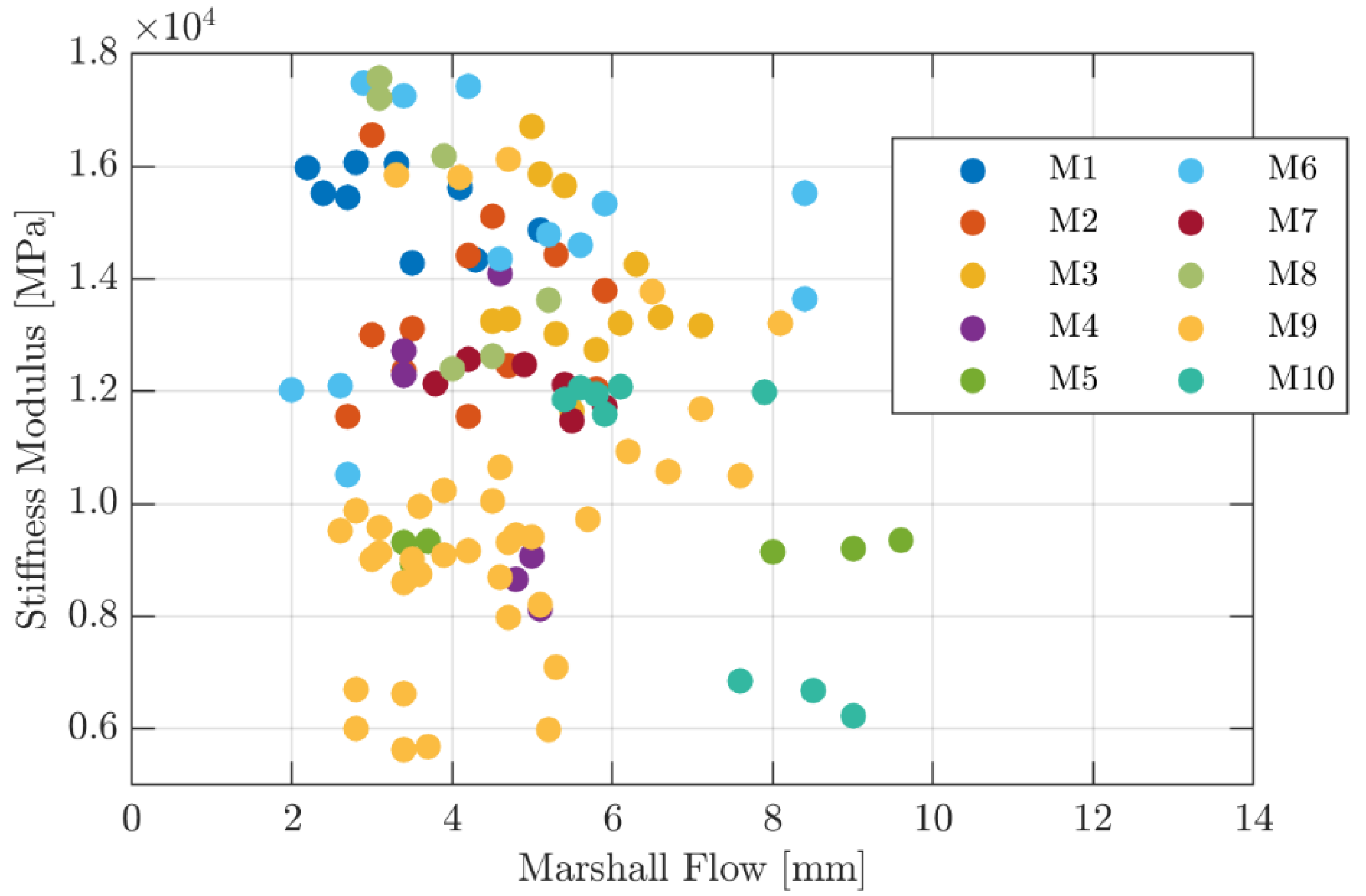
In Section 3.3 a detailed analysis of the correlation strength between the Marshall mechanical parameters and stiffness is presented. However, the scatter plot suggesting the type of correlation between stiffness modulus and Marshall stability (or Marshall flow) is presented in Figure 1 (and Figure 2, respectively): the stiffness seems to have some dependence on the Marshall stability, whereas no dependence was found for the flow (please refer to Table 1 for Legend understanding).
Table 1 provides data about HMAC stiffness at 15 °C. Six mixtures showed lower values than the minimum requirement from the specification TP 151—variant VMT 22 with 20% RA (PKB-A), VMT 22 (SK-4), VMT 22 (TPA-3), VMT 22 (TP-5), VMT 22 (SK-5), and VMT 22 (TP-7). For three of them, the values are very low. Additionally, except the VMT 22 with 20% RA (PKB-A) where the stiffness could be influenced by the used 50/70 paving grade, the remaining 5 mixtures with low stiffness were all designed and produced with PMB. Often for HMACs with PMB 25/55-60, it is challenging to exceed the limit of 9000 MPa due to the elastic behavior of this polymer-modified binder, and several optimizations and modifications of the grading curve are needed. This might explain why most variants with lower stiffness are at the same time containing this type of PMB.

3. Methodology

3.1. Shallow Neural Networks with Backpropagation Algorithm

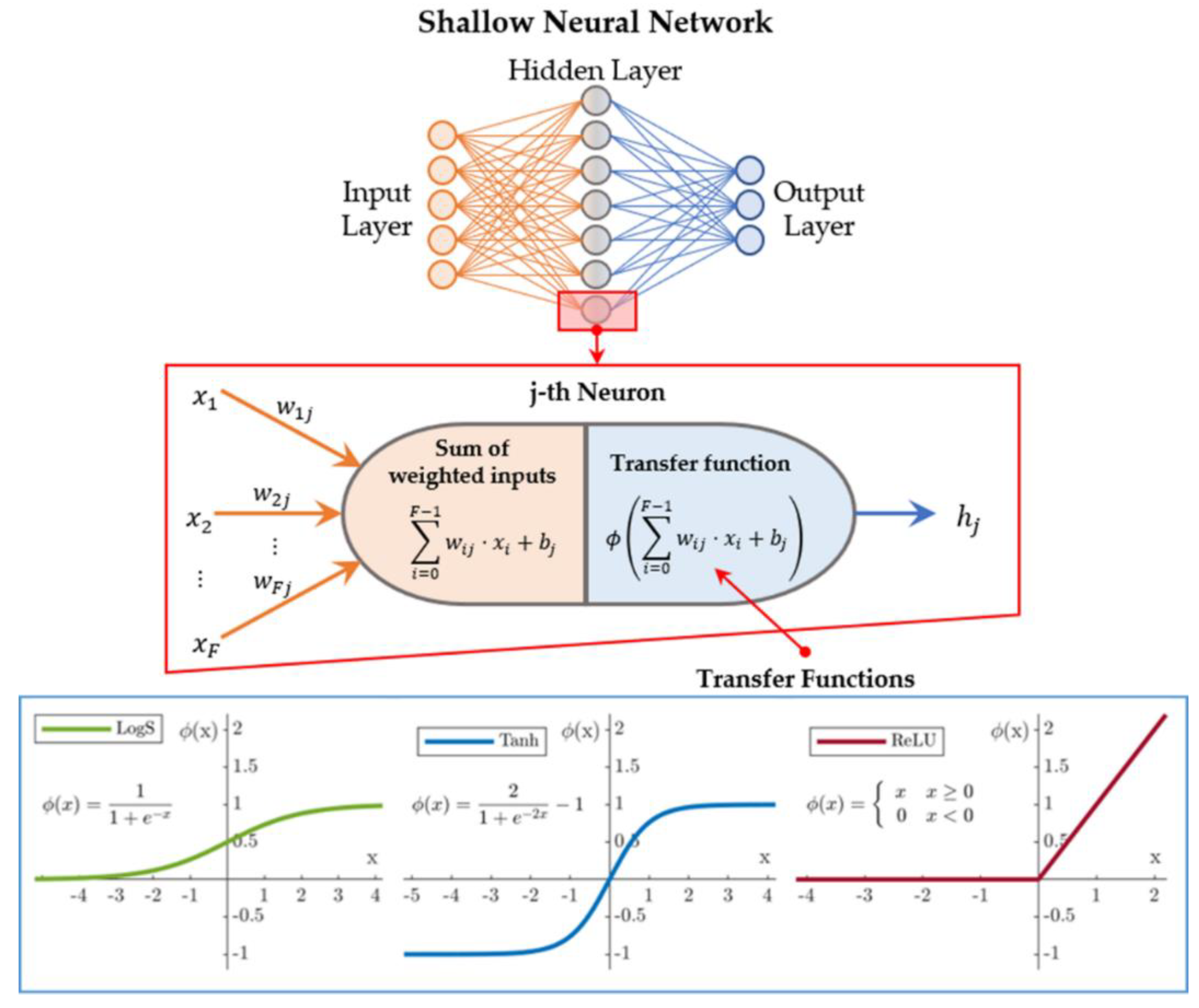
Shallow Neural Networks (SNNs), also called Multilayer Perceptron Neural Networks (MLPs), is a type of Artificial-Intelligence-based on the feedforward network architecture, which can approximate essentially any relation between input and output patterns to an arbitrary degree of accuracy [40,41]. To fully understand the topology and algorithmic functioning of an SNN, the reader should be reminded that the biological nervous system, the brain, acquires knowledge and abilities by a learning process, and that specific synaptic weights of interneuron’s connections store the acquired know-how to replicate it. Similarly, to perform a particular task or function of interest, a Shallow Neural Network has to be trained using a process, typically supervised (i.e., based on input pattern x R F and ground-truth target y R known beforehand), that iteratively updates connections’ weights, according to a learning rule, until the network is able to replicate the desired task with the required accuracy. In fact, a Multilayer Perceptron Neural Networks consists of an input layer, at least one hidden layer, and an output layer. Each of these layers has several processing units, the artificial neurons, and each of them is interconnected with weighted connections to any other unit in the subsequent layer: thereby, the information to be processed travels in just one direction, from input to output layer. Figure 3 shows a typical SNN topology.
Artificial neurons perform the network computations: these are logistic regression models with a nonlinear activation function. This means that each neuron in the first hidden layer implements a dot product between the input feature vector x R F and the vector w j ( 1 ) R F that represents the weights of the connections it has made with each component of the input feature vector (or the neurons x i ) and adds a scalar bias b j ( 1 ) . The resulting scalar is passed to a function ϕ ( 1 ) , called transfer or activation unit, which returns the neuron’s output: h j ( 1 ) = ϕ ( 1 ) ( i = 0 F 1 w i j ( 1 ) x i + b j ( 1 ) ) . Some activation functions, which are also employed in this study, are shown in Figure 3: the rectified linear (ReLU), the hyperbolic tangent (TanH), and the logistic sigmoid (LogS) units. The first hidden layer output is the vector h ( 1 ) = [ h 0 ( 1 ) , , h N 1 ( 1 ) ] , with N the number of neurons that form the layer itself, but it is also the input vector of the subsequent hidden layer. Therefore, the outlined process is repeated until the output of the network is computed: y ^ = ϕ ( o u t ) ( h ( L ) ) . The matrix W = { w i j ( l ) , b j ( l )   |   l   { 1 , 2 , , L } } , with L the number of network layers, forms the set of parameters to be defined in the supervised training process, in which a back-propagation algorithm is typically used [42]. These algorithms compute the first-order approximation of the gradients of a loss metric L ( y ^   , y ) (or error function), between the network output y ^ and the expected target vector y , with respect to the parameters W ; then, a learning rule uses the derivatives of L ( ) to correct the weights and biases of the network, performing several iterations until the loss value is minimized; the resulting parameters are kept fixed to process new feature patterns. In this study, the loss optimization objective L ( ) is the Mean Squared Error (MSE):
L ( y ^ ( W e ) , y , W e ) = 1 M m = 1 M ( y ^ m ( W e ) y m ) 2
where W e is the parameters’ matrix at iteration e of the training process and y ^ ( W e ) y the errors of the corresponding network, whereas M is the number of observations in the training set. In fact, since a single experimental data set is usually available, it is randomly partitioned, according to fixed percentages, into a training, a validation, and a test subset: this practice is known as the hold-out method.
The training set contains the data used to train the SNN, while the validation and test sets hold the data intended to evaluate the model’s effectiveness. Evaluation on the validation set occurs at regular intervals during the training process, while the test set evaluation is typically performed on the fully trained model when it is desired to estimate the model’s generalization capability (i.e., the out-of-sample performance) and then to compare the accuracy of different models. In fact, generalization refers to how well the concepts learned by a Machine Learning model apply to specific observations not used by the neural network during the training process since the model, in order to minimize the MSE, might fit too much of the training data. Such a situation, known as Overfitting, is caused by large values of the connections’ weights and results in an excessively fluctuating and physically unjustified interpolating surface/curve of the experimental data. A good generalization, stated on the basis of a given performance metric’s value, allows reliable predictions to be made in the future about data out of the training sample, since the overfitting problem has been successfully prevented. In particular, among the methods to avoid overfitting and improve generalization, Early Stopping is the most widely used and simplest approach [41]. This method exploits the iterative nature of the training process and the validation data set to decide when to stop the training, according to a procedure called cross-validation: in fact, at each iteration of the training algorithm, the performance of the training process can be measured by monitoring the model error on the validation set. In general, it is observed that up to a certain number of iterations, new iterations improve the model. However, after that point, the model’s capability to generalize can weaken as the neural network begins to overfit the training data and compromise the accuracy of the validation set. When the error on the validation set goes up for several iterations (i.e., in this study, for 7 iterations), the training is stopped, and the weights and biases that produced the minimum MSE on the validation data set are employed as the final trained network parameters.
In the current study, the Levenberg-Marquardt backpropagation algorithm [43], jointly with the Early Stopping method, was employed due to its efficiency in training Shallow Neural Networks among those implemented in MATLAB® [41]. In order to ensure convergence to the minimum of the error surface (and thus to the optimum values of the connections’ weights), the training process was repeated 10 times and the best performing model was selected. With regard to the hold-out method, it is worth pointing out that such a practice has two major drawbacks when the number of observations is small: first, some relevant patterns may be excluded from the training set; second, the training-test splitting makes the model sensitive to the randomness of data in the training set. Therefore, since the purpose of the study is to predict the representative mechanical response of each asphalt concrete considered here, the original data set was augmented by Q = 38 data by averaging the experimental results of specimen replicas of each HMAC variant and associating the main mix composition features of the original variant with each new synthetic target. The obtained stiffness modulus values form a representative set of all situations for which the network will be used. For this reason and to avoid the aforementioned problems, the cross-validating (20%) and the training (80%) sets for the SNN training procedure were selected randomly from the experimental data set (115 Marshall test specimens), while the 38 synthetic data were used for testing the trained SNN model.

3.2. Bayesian Optimization

The definition of the neural network topology and of the training algorithm parameters (i.e., the model’s hyper-parameters) is an essential step in the application of any Machine Learning approach to a specific input-output fitting problem. This process, known as hyper-parameters tuning, represents a challenge for any research engineer and is closely related to model selection, since the hyper-parameters determine the response of the neural network and therefore the performance of the model of which they are part. However, this tuning process is simplified when dealing with Shallow Neural Networks: Hagan et al. [41] assert that an SNN, as defined in the previous Paragraph, can arbitrarily well solve any multidimensional regression problem between given data by providing a sufficient number of neurons and an adequate transfer function to its single hidden layer. It means that the SNN hyper-parameters, when the parameters of the Levenberg-Marquardt training algorithm are set to their default values (please refer to the LM algorithm implementation proposed by the MathWorks® within the well-known MATLAB® ANN Toolbox), are related only to the network architecture, namely the number N of neurons that form the hidden layer and the activation unit ϕ that characterizes them. Therefore, it becomes clear that the choice to exploit SNNs stems from the possibility of simplifying the hyper-parameters tuning problem as well as from the need to identify an easily interpretable and usable modeling tool for the research engineer or laboratory technician interested in the development of predictive models of the asphalt concrete’s mechanical response. Figure 4 shows a flowchart of the optimization procedure followed in this study.
Regarding strategies for carefully defining model hyper-parameters, standard approaches involve a random or grid search for the optimal set within pre-defined ranges on the basis of a sampling method. However, there are many optimization algorithms available nowadays that can reduce the time spent in searching for the best model hyperparameters. Among them, the Bayesian optimization (BO) algorithm [44] has found considerable success mainly due to the work of Snoek et al. [45]. The goal of the optimization process is to minimize a given objective function f ( z ) for z = [ z p   ] , p { 0 , , P } , P N in a bounded domain Z p R . For this purpose, the BO algorithm adopts a Gaussian Process regression model (GPR) for f ( z ) [46], i.e., builds a non-parametric probabilistic model of the objective function, and updates it based on Bayesian statistics for each new evaluation of f ( z ) . Then, an acquisition function a ( z ) based on the prior distribution is maximized to determine the next point z n e x t for the evaluation: z n e x t = a r g m a x z a ( z ) . By repeating this procedure iteratively (until the set maximum number of iterations is reached), the BO algorithm progressively improves the underlying probabilistic model for the objective function and thereby allows the acquisition function to sample points that improve the metric f ( z ) . For optimal results, a rule of thumb asserts to set a maximum number of runs greater than or equal to 20 times the number of hyper-parameters to be optimized. In particular, the acquisition function best known for its capability to efficiently reduce the number of evaluations required to find the global minimum of many black-box functions [47,48] is the Expected Improvement (EI) algorithm [49]. Such EI function evaluates the goodness of a point z by the expected amount of improvement in f ( z ) , ignoring the solutions that cause an increase in the objective metric. To escape a local minimum, the correction proposed by Bull [50] allows the EI acquisition function to modify its behavior when it estimates the over-exploitation of an area of the bounded domain Z p : the resulting acquisition function is called Expected-Improvement-Plus (EIP) and it has been used in the current study setup.
Focusing on the current problem, namely the modeling of high-modulus asphalt concrete stiffness by means of Shallow Neural Networks, the objective function has to consider both out-of-sample performances, i.e., generalization capability, and model parsimony. In fact, as the complexity of the network increases (i.e., in this study, as the number of hidden neurons increases), the SNN does not use all of its weights to minimize the mean squared error because early stopping restricts the number of effective parameters, i.e., limits the weights value, to avoid overfitting. This means that if a “large” network was selected for the given problem, it would not necessarily overfit the data (due to early stopping) but it would definitely take longer to compute the network response, which might not be very different from that of a “smaller” network. If this happened, the model would be over-parameterized for the task, with direct consequences on efficiency. Therefore, the function f ( · ) used in this study adds a penalty term, reliant on the number K = 3 N + 1 of network parameters (i.e., weights and biases) and the number M = 92 of observations in the training set, to a term measuring the goodness-of-prediction of the model to the Q = 38 test data [51]:
f ( N , ϕ , y , Q , M ) = log ( 1 Q q = 1 Q ( y ^ q ( N , ϕ ) y q ) 2 ) + 2 ( 3 N + 1 ) M
Given the P = 2 hyperparameters, N and ϕ , and fixed their ranges Z N = { 1 , , 20 } , Z ϕ = { T a n H , R e L U , L o g S } , f ( ) is a function that implements an SNN with N neurons in its hidden layer and ϕ as activation function; such SNN is trained on a M -observation training set for 10 times and early stopped each time to avoid overfitting; the best performing SNN is then selected and performs on a Q test data set; f ( ) returns a single scalar that expresses the balance between model generalization and model parsimony. The Bayesian optimization algorithm is run for 40 iterations. The optimal hyper-parameters N and ϕ , and then the optimal model, are selected when f ( ) is minimized by the BO algorithm.
All codes required for this study were implemented in MATLAB® using the ANN Toolbox framework and they were run on a machine provided with an Intel® Core™ i7-6700HQ 2.60 GHz CPU and 16GB of RAM running Windows 10 Home. Each experiment lasted about 2 h.

3.3. Input Features Selection and Models Evaluation

Recalling that the aim of the study is to develop a model for predicting the stiffness modulus of different asphalt concretes, the problem arises of selecting the input variables or features that will characterize the model itself. In fact, a model that engages irrelevant features, poorly correlated with the target variable, may have learning difficulties, higher memory requirements, and increased complexity, as well as worse prediction accuracy and then poor generalization capability [52,53]. Due to the dependency of mechanical characteristics on both aggregate and bitumen properties, it is important to include the fundamental parameters of asphalt concretes related to their composition in the input feature vector, i.e., in the current study, the bitumen content (% by mass of mix), the air voids content (%), maximum and average bulk density (g/cm3), along with a categorical variable that distinguishes the bitumen type and RAP percentages (values from 0 to 10). Nevertheless, the use of the Marshall test results, in terms of Stability or Quotient, as predictors could help to improve the accuracy of the predictions, even though these parameters are often considered as target variables due to their frequent use in the mix design process or simply due to the implied costs of the test [54,55,56]. In particular, the relationship between Marshall Stability (MS), as well Marshall Quotient (MQ), and Stiffness Modulus was investigated using the non-parametric Spearman Rank Order Correlation (rho) [57]. There was a strong correlation between MS and Stiffness ( r h o = 0.67 ,   n = 115 ,   p < 0.0005 ) , with high stiffness levels associated with high stability levels, and the same applies to the relationship between MQ and Stiffness but with a medium correlation strength ( r h o = 0.35 ,   n = 115 ,   p < 0.0005 ) .
Therefore, three SNNs characterized by a different number of predictors were developed in this study and referred to in the following with the acronyms MIXSNN, MSSNN, MQSNN. More specifically, the first of these employs the aforementioned five mix composition variables to predict the Stiffness Modulus, while the remaining ones add MS and MQ to the input feature vector, respectively. Each variable belonging to both input and target vector has been standardized before being processed by the SNN, i.e., all variables have been rescaled to have zero mean and unity standard deviation: such an adjustment served to improve the efficiency of the Levenberg-Marquardt algorithm. In addition, all three models were optimized according to the procedure reported in Section 3.2, and then, evaluated and compared on the test data set using statistical performance metrics to identify the features combination that yields the best generalization capability. The employed model evaluation functions are the mean absolute error (MAE), the root mean square error (RMSE), the coefficient of determination (R2), and adjusted R-squared (R2adj). For a detailed description of each performance metric please refer to Biecek and Burzykowski [58], as well Legates and McCabe [59].
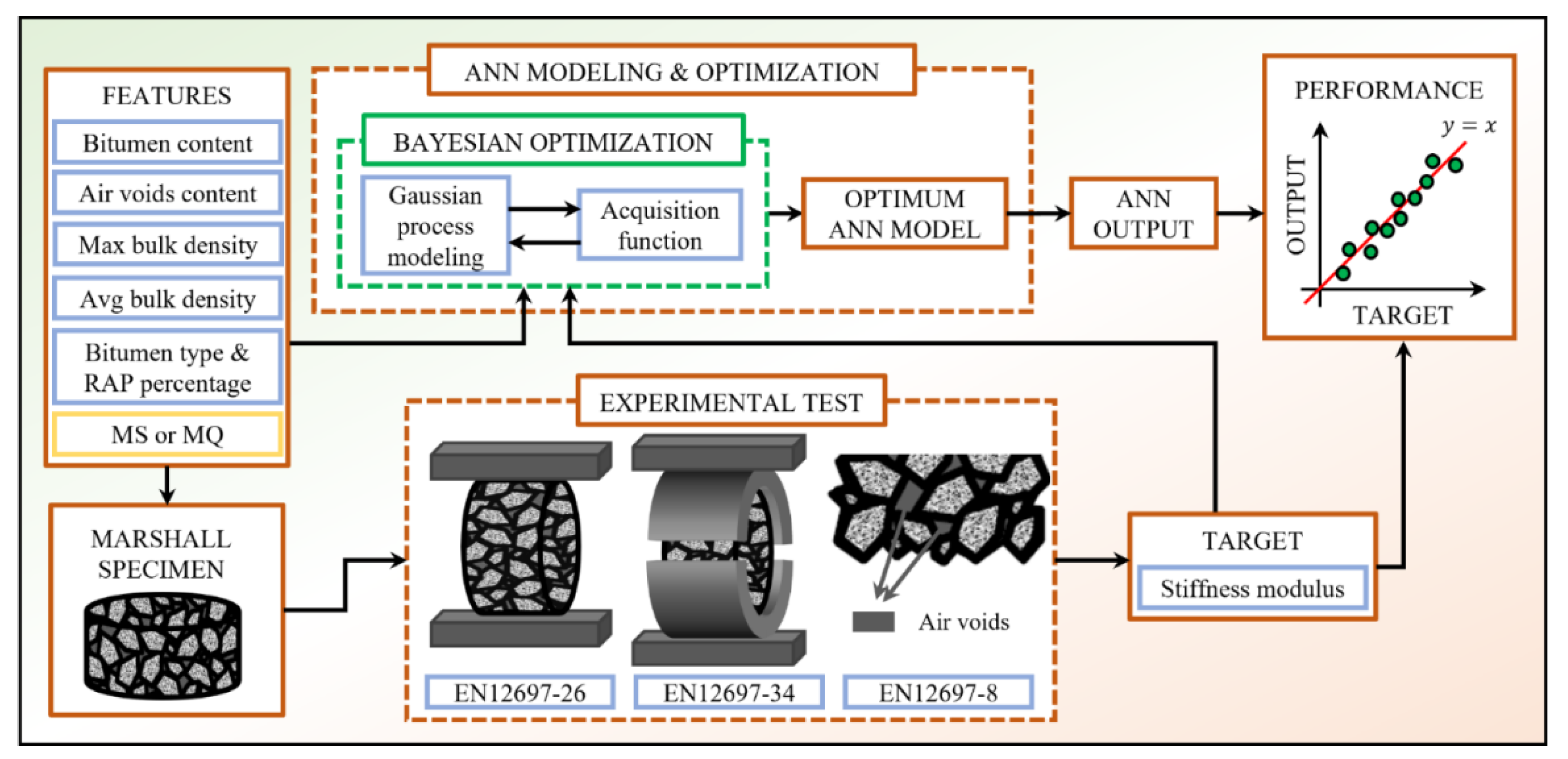
In summary, the investigated SNNs is realized with a 5- or 6-neurons input layer (one neuron for each input feature), a N -neurons hidden layer whose processed output is passed to an activation unit ϕ (⋅) being either a ReLU, TanH or LogS function, and a 1-neuron output layer associated with the identity activation function. Figure 5 shows a summary flowchart of the full procedure followed.

4. Discussion

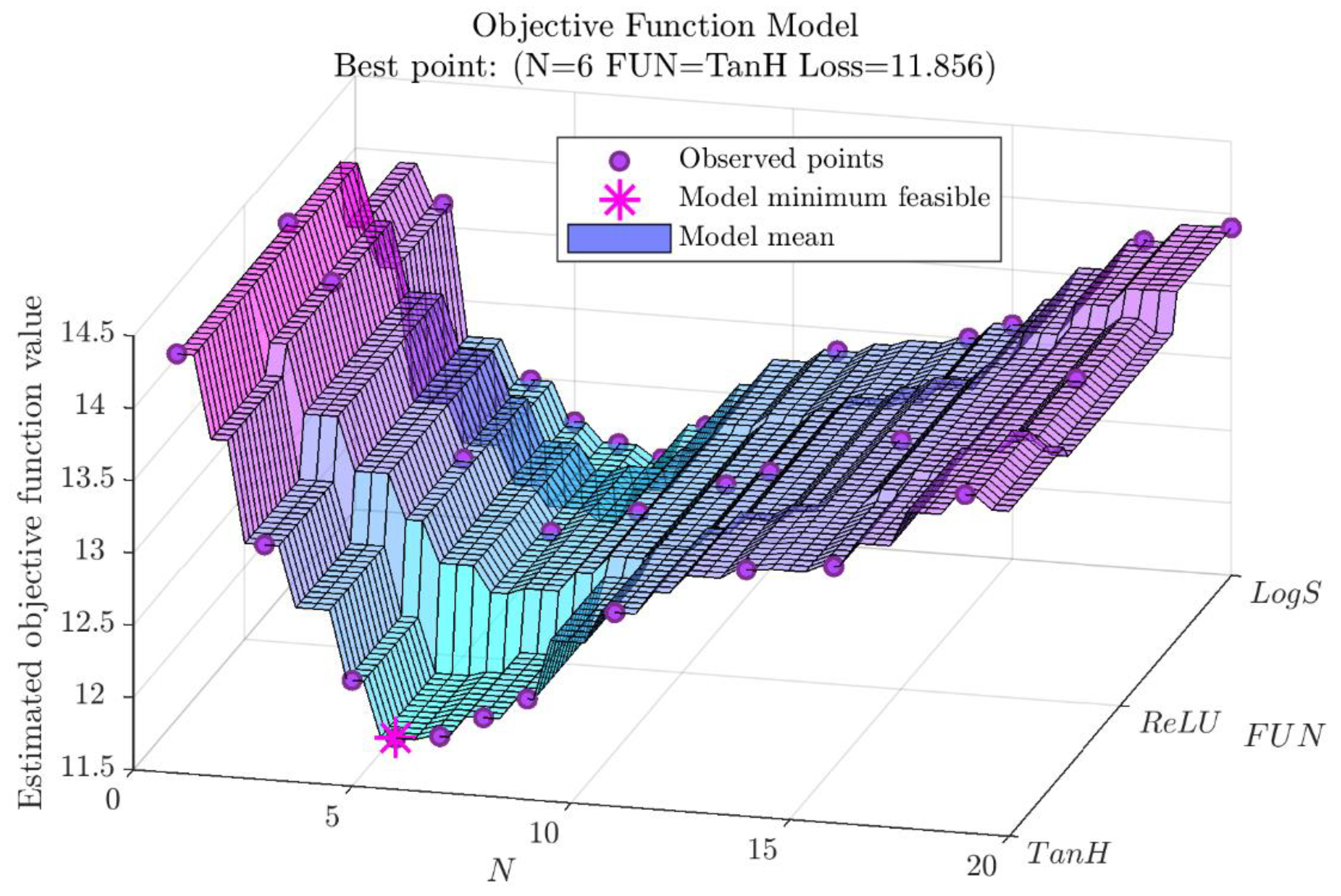
Table 2 summarizes the results of the hyperparameter optimization process, according to the procedure described in Section 3.2, for each group of input features and the value of the statistical metrics assessing generalization capability for each model. In particular, columns 3 and 4 show the number of neurons and the activation function of the hidden layer, identified by the Bayesian process based on the objective function f ( ) , for the three SNNs (i.e., MIXSNN, MSSNN, MQSNN): these shallow solutions ( N < 8 neurons) represent the most efficient neural configuration for each modeling problem considered (Section 3.3). The best result in terms of f ( ) (fifth column of Table 2) was achieved by the MSSNN ( f ( ) = 11.856 , Table 2), i.e., the network that receives as input features the Marshall Stability along with the mix composition parameters of the HMAC: Figure 6 shows the Gaussian Process regression model (overlapped with the objective function points that were sampled) that the Bayesian optimizer has progressively developed to find the minimum of the function f ( ) for the MSSNN. This network, which is the best in terms of generalization performance (last four columns of Table 2), receives as input a 6-component features vector, which is processed by a 6-neurons hidden layer characterized by the TanH activation function.
In general, the addition of the empirical mechanical parameters among the predictors of the stiffness modulus improved the prediction accuracy compared to the use of mixes’ composition parameters alone, as shown by the model evaluation functions: in particular, the values of the R2adj parameter (last column of Table 2), a modified version of R2 which assesses the effect of adding predictors to a model, increase with the use of MS or MQ, showing that the new independent term improves the model more than would be expected by chance, but the percentage gain in model accuracy is really paltry. In fact, although the percentage variation in MAE between MIXSNN and MSSNN is +23.4%, in terms of R2adj the gain is only +0.29% and therefore such that it may not justify the use of additional data, such as any results of the Marshall test. Therefore, even though in the following the results of the MSSNN will be presented as it represents the best model among those evaluated, it is advised to use the Marshall parameters when the prediction of the IT-CY asphalt mix stiffness from the main composition parameters of the HMACs should not be satisfactory.
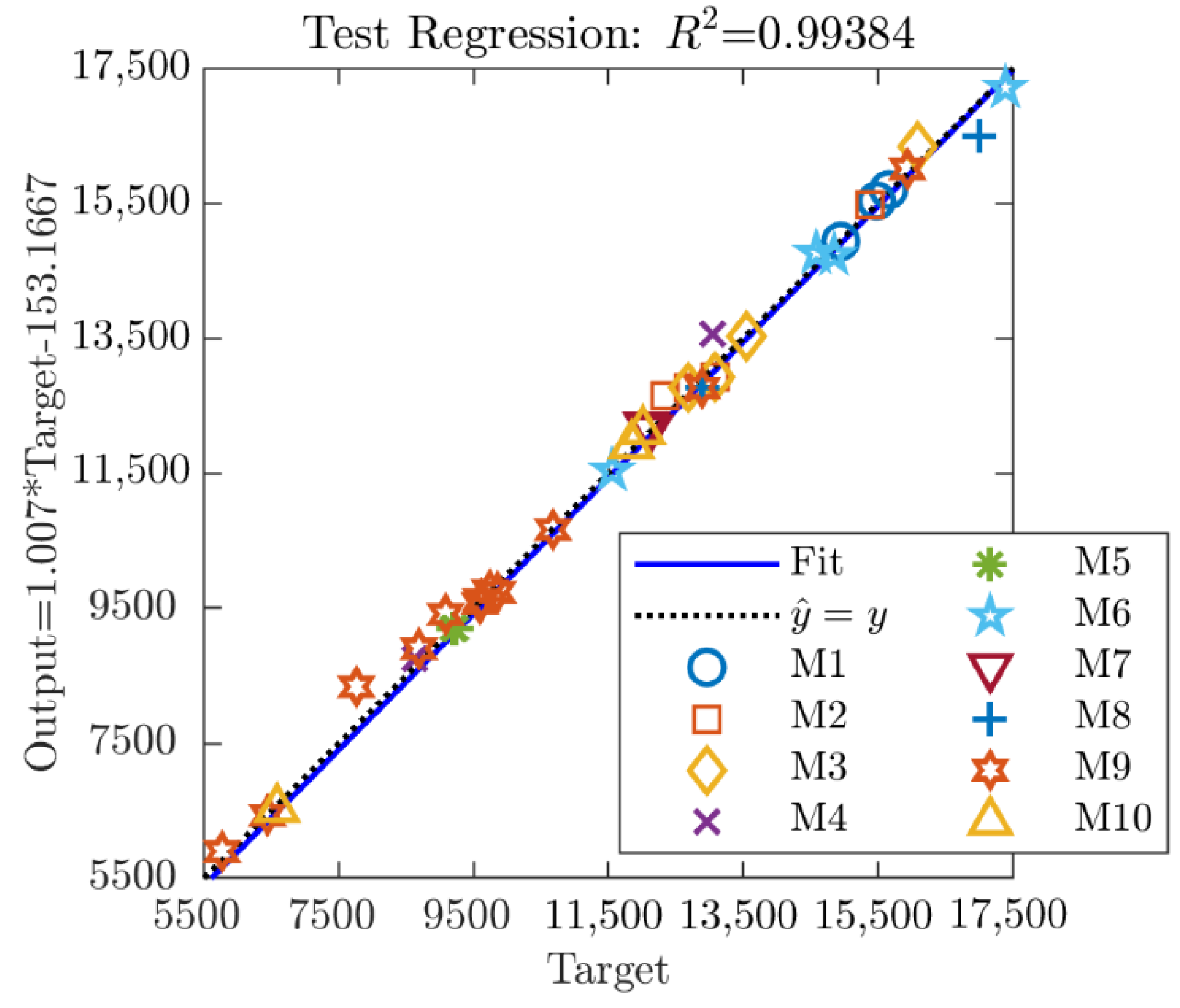
Figure 7 shows the linear regression model between the network outputs and the experimental targets in the test data set: the high value of the coefficient of determination R2 = 0.99384, very close to unity, suggests that the MSSNN is capable of accurately predicting the average mechanical response of HMAC specimen replicas in the training data set and that the problem of overfitting has been avoided despite the small data set available. The same is true for the other SNNs, which show slightly lower performance (please refer to the second-to-last column of Table 2). Therefore, the data augmentation approach designed and implemented in the present study has been particularly suitable for the modeling problem in question and represents an effective approach whenever multiple replicates of different mixtures were available and it was desired to model the average mechanical response resulting from different aggregate compositions, binder percentages, and so on. The Stiffness-Stability comparison between network outputs and experimental targets in the training data set is presented in Figure 8: the absence of an exact matching between the blue and orange points is further evidence of the MSSNN’s capability to disregard the behavior of the single replica in order to capture the average mechanical response resulting from the mixtures’ composition parameters.
Finally, it is necessary to point out that, generally, the data sets used for modeling the mechanical behavior of ACs are relatively small, due to the time and cost that the execution of a multitude of laboratory tests on multiple replicas of the same mixture and/or different variants implicitly requires. Therefore, even though the experimental data set exploited in this paper may seem limited for neural network modeling, there is evidence that the application of shallow neural networks, coupled with an appropriate data augmentation technique, avoids model overfitting and, consequently, an effective procedure for small HMACs data sets has been validated. Accordingly, there is the possibility of extending the current study (using the same techniques) to other mixtures, characterized by binders and aggregates different from those considered.

5. Conclusions

The following conclusions can be drawn from this study:
  • The IT-CY Stiffness Modulus of 115 Marshall test specimens of high-modulus asphalt mixtures prepared in the laboratory with reclaimed asphalt pavement or polymer-modified bitumen has been investigated, according to EN 12697-26 Annex C, as part of real case-mix design processes.
  • There were good correlation strengths between the Stiffness Modulus and the Marshall test results, with high stiffness levels associated with high stability or quotient levels. Therefore, one of these empirical parameters could be used as an input feature, along with some parameters related to the HMAC composition, to improve the performance of a predictive model.
  • Machine Learning approaches have been employed for the development of a predictive model of the HMACs’ stiffness modulus: the focus was particularly on Shallow Neural Networks, given their simple structure and good computational power even with respect to small data sets.
  • A Bayesian optimization process was used to identify the neural topology, as well as the transfer function, optimal for the required modeling. In addition, a data augmentation strategy was designed for the case of the IT-CY test.
  • By employing different performance metrics, it was possible to compare the optimal models obtained by varying the input feature related to the empirical Marshall test results. The SNN, which showed the best prediction accuracy of the average mechanical response of HMAC variants, receives as input a 6-component features vector, i.e., the Marshall stability (kN), the bitumen content (% by mass of mix), the air voids content (%), maximum and average bulk density (g/cm3), along with a categorical variable that distinguishes the bitumen type and RAP percentages (values from 0 to 10); such input features vector is processed by 6 neurons in the hidden layer characterized by a hyperbolic tangent activation unit.
  • A worthwhile future development could be an in-depth investigation of aggregate grading curves’ influence on stiffness predictions by including additional inputs connected with mixture proportion. Another valuable alternative would be to replace during the modeling phase, variables referring to empirical properties (i.e., Marshall Stability) with those referring to pavement performance. In this way, it would be possible to predict by machine learning approaches fatigue life and/or permanent deformation resistance. Such an attempt would represent a significant step toward performance-based mixture design.

Author Contributions

Conceptualization, N.B., M.M. and J.V.; methodology, N.B., M.M., F.R., J.V. and P.V.; software, M.M.; validation, N.B., M.M., F.R., J.V. and E.M.; formal analysis, N.B., M.M., F.R., J.V., P.V. and E.M.; investigation, J.V. and P.V.; resources, N.B. and J.V.; data curation, N.B., M.M., F.R., J.V., P.V. and E.M.; writing—original draft preparation, N.B., M.M., F.R., J.V., P.V. and E.M.; writing—review and editing, N.B., M.M., F.R., J.V., P.V. and E.M.; visualization, E.M.; supervision, N.B.; project administration, N.B. and J.V.; funding acquisition, N.B. and J.V. All authors have read and agreed to the published version of the manuscript.

Funding

This research received no external funding.

Institutional Review Board Statement

Not applicable.

Informed Consent Statement

Not applicable.

Data Availability Statement

The data presented in this study are available in Table 1 of the current paper.

Conflicts of Interest

The authors declare no conflict of interest.

References

  1. Espersson, M. Effect in the high modulus asphalt concrete with the temperature. Constr. Build. Mater. 2014, 71, 638–643. [Google Scholar] [CrossRef]
  2. Miró, R.; Valdés, G.; Martínez, A.; Segura, P.; Rodríguez, C. Evaluation of high modulus mixture behaviour with high reclaimed asphalt pavement (RAP) percentages for sustainable road construction. Constr. Build. Mater. 2011, 25, 3854–3862. [Google Scholar] [CrossRef]
  3. Rys, D.; Judycki, J.; Pszczola, M.; Jaczewski, M.; Mejlun, L. Comparison of low-temperature cracks intensity on pavements with high modulus asphalt concrete and conventional asphalt concrete bases. Constr. Build. Mater. 2017, 147, 478–487. [Google Scholar] [CrossRef]
  4. Corté, J.F. Development and uses of hard-grade asphalt and of high-modulus asphalt mixes in France. Transp. Res. Circ. 2001, 503, 12–31. [Google Scholar]
  5. Newcomb, D.E.; Willis, R.; Timm, D.H. Perpetual Asphalt Pavements—A Synthesis; Asphalt Pavement Association of Michigan: Okemos, MI, USA, 2002. [Google Scholar]
  6. Geng, H.; Clopotel, C.S.; Bahia, H.U. Effects of high modulus asphalt binders on performance of typical asphalt pavement structures. Constr. Build. Mater. 2013, 44, 207–213. [Google Scholar] [CrossRef]
  7. Marvila, M.T.; Azevedo, A.R.G.; Alexandre, J.; Zanelato, E.B.; Azeredo, N.G.; Simonassi, N.T.; Monteiro, S.N. Correlation between the properties of structural clay blocks obtained by destructive tests and Ultrasonic Pulse Tests. J. Build. Eng. 2019, 26, 100869. [Google Scholar] [CrossRef]
  8. Pasetto, M.; Baldo, N. Re-use of industrial wastes in cement bound mixtures for road construction. Environ. Eng. Manag. J. 2018, 17, 417–426. [Google Scholar] [CrossRef]
  9. Wang, L.; Song, Z.; Zeng, S.; Liu, J.; Ma, K. Exploration of the load fatigue test method for cement concrete wheels. Case Stud. Constr. Mater. 2022, 16, e00793. [Google Scholar] [CrossRef]
  10. Lee, H.J.; Lee, J.H.; Park, H.M. Performance evaluation of high modulus asphalt mixtures for long life asphalt pavements. Constr. Build. Mater. 2007, 21, 1079–1087. [Google Scholar] [CrossRef]
  11. Moghaddam, T.; Baaj, H. Rheological characterization of high-modulus asphalt mix with modified asphalt binders. Constr. Build. Mater. 2018, 193, 142–152. [Google Scholar] [CrossRef]
  12. Si, C.; Zhou, Y.; You, Z.; He, Y.; Chen, E.; Zhang, R. Micro-mechanical analysis of high modulus asphalt concrete pavement. Constr. Build. Mater. 2019, 220, 128–141. [Google Scholar] [CrossRef]
  13. Zaumanis, M.; Arraigada, M.; Poulikakos, L.D. 100% recycled high-modulus asphalt concrete mixture design and validation using vehicle simulator. Constr. Build. Mater. 2020, 260, 119891. [Google Scholar] [CrossRef]
  14. Baldo, N.; Valentin, J.; Manthos, E.; Miani, M. Numerical Characterization of High Modulus Asphalt Concrete Containing RAP: A Comparison among Optimized Shallow Neural Models. In IOP Conference Series: Materials Science and Engineering, Proceedings of the 5th World Multidisciplinary Civil Engineering-Architecture-Urban Planning Symposium, Prague, Czech Republic, 15–19 June 2020; IOP Publishing: Bristol, UK, 2020. [Google Scholar] [CrossRef]
  15. Yun, T.; Kim, Y.R. Viscoelastoplastic modeling of the behavior of hot mix asphalt in compression. KSCE J. Civ. Eng. 2013, 17, 1323–1332. [Google Scholar] [CrossRef]
  16. Di Benedetto, H.; Sauzéat, C.; Clec’h, P. Anisotropy of bituminous mixture in the linear viscoelastic domain. Mech. Time-Depend. Mater. 2016, 20, 281–297. [Google Scholar] [CrossRef]
  17. Rahmani, E.; Darabi, M.K.; Little, D.N.; Masad, E.A. Constitutive modeling of coupled aging-viscoelastic response of asphalt concrete. Constr. Build. Mater. 2017, 131, 1–15. [Google Scholar] [CrossRef]
  18. Darabi, M.K.; Huang, C.W.; Bazzaz, M.; Masad, E.A.; Little, D.N. Characterization and validation of the nonlinear viscoelastic-viscoplastic with hardening-relaxation constitutive relationship for asphalt mixtures. Constr. Build. Mater. 2019, 216, 648–660. [Google Scholar] [CrossRef]
  19. Specht, L.P.; Khatchatourian, O.; Brito, L.A.T.; Ceratti, J.A.P. Modeling of asphalt-rubber rotational viscosity by statistical analysis and neural networks. Mater. Res. 2007, 10, 69–74. [Google Scholar] [CrossRef]
  20. Mirzahosseini, M.R.; Aghaeifar, A.; Alavi, A.H.; Gandomi, A.H.; Seyednour, R. Permanent deformation analysis of asphalt mixtures using soft computing techniques. Expert Syst. Appl. 2011, 38, 6081–6100. [Google Scholar] [CrossRef]
  21. Androjić, I.; Marović, I. Development of artificial neural network and multiple linear regression models in the prediction process of the hot mix asphalt properties. Can. J. Civ. Eng. 2017, 44, 994–1004. [Google Scholar] [CrossRef]
  22. Alrashydah, E.I.; Abo-Qudais, S.A. Modeling of creep compliance behavior in asphalt mixes using multiple regression and artificial neural networks. Constr. Build. Mater. 2018, 159, 635–641. [Google Scholar] [CrossRef]
  23. Ziari, H.; Amini, A.; Goli, A.; Mirzaiyan, D. Predicting rutting performance of carbon nano tube (CNT) asphalt binders using regression models and neural networks. Constr. Build. Mater. 2018, 160, 415–426. [Google Scholar] [CrossRef]
  24. Montoya, M.A.; Haddock, J.E. Estimating asphalt mixture volumetric properties using seemingly unrelated regression equations approaches. Constr. Build. Mater. 2019, 225, 829–837. [Google Scholar] [CrossRef]
  25. Baldo, N.; Manthos, E.; Pasetto, M. Analysis of the mechanical behaviour of asphalt concretes using artificial neural networks. Adv. Civ. Eng. 2018, 2018, 1650945. [Google Scholar] [CrossRef] [Green Version]
  26. Ozsahin, T.S.; Oruc, S. Neural network model for resilient modulus of emulsified asphalt mixtures. Constr. Build. Mater. 2008, 22, 1436–1445. [Google Scholar] [CrossRef]
  27. Tapkın, S.; Çevik, A.; Uşar, Ü. Accumulated strain prediction of polypropylene modified marshall specimens in repeated creep test using artificial neural networks. Expert Syst. Appl. 2009, 36, 11186–11197. [Google Scholar] [CrossRef]
  28. Saoudi, B.S.; Haddadi, S.H. Predicting creep deformation of asphalts modified with polymer using artificial neural networks. Mag. Civ. Eng. 2021, 101, 10106. [Google Scholar] [CrossRef]
  29. Xiao, F.; Amirkhanian, S.; Juang, C.H. Prediction of fatigue life of rubberized asphalt concrete mixtures containing reclaimed asphalt pavement using artificial neural networks. J. Mater. Civ. Eng. 2009, 21, 253–261. [Google Scholar] [CrossRef]
  30. Ahmed, T.M.; Green, P.L.; Khalid, H.A. Predicting fatigue performance of hot mix asphalt using artificial neural networks. Road Mater. Pavement Des. 2017, 18, 141–154. [Google Scholar] [CrossRef]
  31. Ceylan, H.; Schwartz, C.W.; Kim, S.; Gopalakrishnan, K. Accuracy of predictive models for dynamic modulus of hot-mix asphalt. J. Mater. Civ. Eng. 2009, 21, 286–293. [Google Scholar] [CrossRef] [Green Version]
  32. Gong, H.; Sun, Y.; Dong, Y.; Han, B.; Polaczyk, P.; Hu, W.; Huang, B. Improved estimation of dynamic modulus for hot mix asphalt using deep learning. Constr. Build. Mater. 2020, 263, 119912. [Google Scholar] [CrossRef]
  33. Zavrtanik, N.; Prosen, J.; Tušar, M.; Turk, G. The use of artificial neural networks for modeling air void content in aggregate mixture. Autom. Constr. 2016, 63, 155–161. [Google Scholar] [CrossRef]
  34. Hussain, F.; Ali, Y.; Irfan, M. Quantifying the Differential Phase Angle Behaviour of Asphalt Concrete Mixtures Using Artificial Neural Networks. Int. J. Pavement Res. Technol. 2021, 121235, 1–19. [Google Scholar] [CrossRef]
  35. Baldo, N.; Manthos, E.; Miani, M. Stiffness modulus and marshall parameters of hot mix asphalts: Laboratory data modeling by artificial neural networks characterized by cross-validation. Appl. Sci. 2019, 9, 3502. [Google Scholar] [CrossRef] [Green Version]
  36. Shahriari, B.; Swersky, K.; Wang, Z.; Adams, R.P.; De Freitas, N. Taking the human out of the loop: A review of Bayesian optimization. Proc. IEEE 2015, 104, 148–175. [Google Scholar] [CrossRef] [Green Version]
  37. Bergstra, J.; Bardenet, R.; Bengio, Y.; Kégl, B. Algorithms for hyper-parameter optimization. In Proceedings of the 25th Annual Conference on Neural Information Processing Systems (NIPS 2011), Granada, Spain, 12–14 December 2011; Neural Information Processing Systems Foundation: La Jolla, CA, USA, 2011; Volume 24. [Google Scholar]
  38. Bergstra, J.; Yamins, D.; Cox, D. Making a science of model search: Hyperparameter optimization in hundreds of dimensions for vision architectures. In Proceedings of the International Conference on Machine Learning, Atlanta, GA, USA, 16–21 June 2013; pp. 115–123. [Google Scholar]
  39. Hoang, V.H.; Nguyen, Q.T.; Tran, A.T.; Tran, T.C.H.; Do, T.A. Mechanical behavior of the asphalt wearing surface on an orthotropic steel bridge deck under cyclic loading. Case Stud. Constr. Mater. 2022, 16, e00836. [Google Scholar] [CrossRef]
  40. Cybenko, G. Approximation by superpositions of a sigmoidal function. Math. Control. Signal Syst. 1989, 2, 303–314. [Google Scholar] [CrossRef]
  41. Demuth, H.B.; Beale, M.H.; De Jess, O.; Hagan, M.T. Neural Network Design; Martin Hagan: Stillwater, OK, USA, 2014. [Google Scholar]
  42. Rumelhart, D.E.; Hinton, G.E.; Williams, R.J. Neurocomputing: Foundations of Research; MIT Press: Cambridge, MA, USA, 1988; pp. 696–699. [Google Scholar]
  43. Hagan, M.T.; Menhaj, M.B. Training feedforward networks with the Marquardt algorithm. IEEE Trans. Neural Netw. 1994, 5, 989–993. [Google Scholar] [CrossRef] [PubMed]
  44. Miani, M.; Dunnhofer, M.; Rondinella, F.; Manthos, E.; Valentin, J.; Micheloni, C.; Baldo, N. Bituminous Mixtures Experimental Data Modeling Using a Hyperparameters-Optimized Machine Learning Approach. Appl. Sci. 2021, 11, 11710. [Google Scholar] [CrossRef]
  45. Snoek, J.; Larochelle, H.; Adams, R.P. Practical Bayesian Optimization of Machine Learning Algorithms. In Proceedings of the 25th International Conference on Neural Information Processing Systems, Lake Tahoe, NV, USA, 13–16 December 2012; pp. 2951–2959. [Google Scholar]
  46. Rasmussen, C.E.; Williams, C.K.I. Gaussian Processes for Machine Learning; MIT Press: Cambridge, MA, USA, 2006. [Google Scholar]
  47. Kushner, H.J. A New Method of Locating the Maximum Point of an Arbitrary Multipeak Curve in the Presence of Noise. J. Basic Eng. 1964, 86, 97–106. [Google Scholar] [CrossRef]
  48. Srinivas, N.; Krause, A.; Kakade, S.M.; Seeger, M. Gaussian Process Optimization in the Bandit Setting: No Regret and Experimental Design. arXiv 2009, arXiv:0912.3995. Available online: https://arxiv.org/abs/0912.3995 (accessed on 11 June 2021).
  49. Mockus, J.; Tiešis, V.; Zilinskas, A. The application of Bayesian methods for seeking the extremum. In Towards Global Optimization, 2nd ed.; Dixon, L.C.W., Szego, G.P., Eds.; North Holland Publishing Co.: Amsterdam, The Netherlands, 1978; pp. 117–129. [Google Scholar]
  50. Bull, A.D. Convergence Rates of Efficient Global Optimization Algorithms. J. Mach. Learn. Res. 2011, 12, 2879–2904. Available online: https://arxiv.org/abs/1101.3501 (accessed on 11 June 2021).
  51. Qi, M.; Zhang, G.P. An investigation of model selection criteria for neural network time series forecasting. Eur. J. Oper. Res. 2001, 132, 666–680. [Google Scholar] [CrossRef]
  52. Bowden, G.J.; Maier, H.R.; Dandy, G.C. Input determination for neural network models in water resources applications. Part 2. Case study: Forecasting salinity in a river. J. Hydrol. 2005, 301, 93–107. [Google Scholar] [CrossRef]
  53. Hastie, T.; Tibshirani, R.; Friedman, J. The Elements of Statistical Learning. Data Mining, Inference, and Prediction, 2nd ed.; Springer: Berlin/Heidelberg, Germany, 2009. [Google Scholar]
  54. Tapkın, S.; Çevik, A.; Uşar, Ü. Prediction of Marshall test results for polypropylene modified dense bituminous mixtures using neural networks. Expert Syst. Appl. 2010, 37, 4660–4670. [Google Scholar] [CrossRef]
  55. Ozgan, E. Artificial neural network based modelling of the Marshall Stability of asphalt concrete. Expert Syst. Appl. 2011, 38, 6025–6030. [Google Scholar] [CrossRef]
  56. Zumrawi, M.M.; Khalill, F.O. Experimental study of steel slag used as aggregate in asphalt mixture. Am. J. Constr. Build. Mater. 2017, 2, 26–32. [Google Scholar] [CrossRef]
  57. Spearman, C. The proof and measurement of association between two things. Am. J. Psychol. 1904, 15, 72–101. [Google Scholar] [CrossRef]
  58. Biecek, P.; Burzykowski, T. Explanatory Model Analysis. Explore, Explain, and Examine Predictive Models; Chapman and Hall/CRC: New York, NY, USA, 2021. [Google Scholar]
  59. Legates, D.R.; McCabe, G.J. A refined index of model performance: A rejoinder. Int. J. Climatol. 2013, 33, 1053–1056. [Google Scholar] [CrossRef]
Figure 1. Scatter plot between Stiffness Modulus and Marshall Stability.
Coatings 12 00054 g001
Figure 2. Scatter plot between Stiffness Modulus and Marshall Flow.
Coatings 12 00054 g002
Figure 3. The SNN topology, the artificial neuron unit, and the main used transfer functions.
Coatings 12 00054 g003
Figure 4. Flow chart of the optimization procedure.
Coatings 12 00054 g004
Figure 5. Step-by-step methodology applied in the current study setup.
Coatings 12 00054 g005
Figure 6. Gaussian Process regression model for the MSSNN.
Coatings 12 00054 g006
Figure 7. Linear regression analysis on the test set for the MSSNN.
Coatings 12 00054 g007
Figure 8. Comparison between experimental target and MSSNN output on the training data set.
Coatings 12 00054 g008
Table 1. Summary of experimental test results and specimens’ characteristics.
MixBitumen TypeIDBulk DensityMax Bulk Density Binder ContentVoids ContentMaximum StrengthMarshall StabilityMarshall FlowIT-CY 15 °C
(g/cm3)(g/cm3)(%)(%)kNkN(0.1 mm)(MPa)
VMT 22 with 30% RA (Froněk-A)20/30M12.4552.6404.97.020.620.03316,062
2.4294.98.022.422.73514,283
2.4564.97.021.623.12816,078
VMT 22 with 30% RA (Froněk-B)20/30M12.4592.6474.67.120.720.95114,867
2.4534.67.319.620.54115,616
2.4564.67.221.021.44314,350
VMT 22 with 30% RA (Froněk-C)20/30M12.4732.6634.37.222.822.42215,974
2.4754.37.024.725.92415,535
2.4854.36.724.124.62715,452
VMT 22 with 20% RA (Froněk-1)20/30M22.4672.6764.37.820.120.55812,049
2.4634.38.019.019.84214,419
2.4614.38.020.221.03013,003
VMT 22 with 20% RA (Froněk-2)20/30M22.4862.6824.67.320.721.75913,792
2.4624.68.218.920.04211,559
2.4804.67.519.619.84712,452
VMT 22 with 20% RA (Froněk-4)20/30M22.4602.6784.98.123.523.55314,441
2.4604.98.124.323.94515,113
2.4434.98.823.924.63016,558
VMT 22 with 20% RA (Froněk-6)20/30M22.4222.6675.29.218.621.83513,116
2.4115.29.619.122.22711,548
2.4225.29.222.325.43412,370
VMT 22 with 30% RA var. 5.150/70M32.5472.6175.12.717.119.77113,171
2.5545.12.417.220.05511,659
2.5385.13.019.621.94513,242
VMT 22 with 30% RA. var. 4.850/70M32.5382.6074.82.617.419.95812,739
2.5354.82.814.816.94713,287
2.5394.82.622.725.56113,217
VMT 22 with 30% RA (Froněk)50/70M32.5492.6024.82.017.420.25313,025
2.5394.82.415.317.96314,267
2.5484.82.116.819.06613,325
VMT 22 with 30% RA (Froněk)50/70M32.5532.6264.62.820.620.75115,871
2.5484.63.018.621.05415,666
2.5484.63.020.223.45016,707
VMT 22 with 20% RA (Froněk-3)50/70M42.4732.6394.86.318.119.03412,729
2.4954.85.420.221.63412,282
2.4774.86.121.522.34614,101
VMT 22 with 20% RA (PKB-A)50/70M42.3972.4964.44.014.213.6488666
2.4214.43.013.413.4509064
2.4124.43.412.212.4518135
VMT 22 with 10% RA (PKB-101)50/70M52.3582.5594.67.912.111.4358950
2.3514.68.115.314.1379339
2.3554.68.012.814.5349311
VMT 22 with 10% RA (PKB-102)50/70M52.3412.5594.58.517.116.2909203
2.3434.58.417.116.1809142
2.3234.59.215.114.2969361
VMT 22 NT20/30M62.3622.4904.75.118.917.14614,357
2.4094.73.221.420.35614,601
2.4094.73.320.819.75214,784
VMT 22 NT20/30M62.2962.4904.77.819.416.38413,653
2.3134.77.120.818.88415,529
2.2964.77.819.716.55915,345
VMT 22 (SK-1)20/30M62.3302.4494.64.925.424.12612,102
2.3244.65.124.523.22012,027
2.3054.65.922.520.52710,528
VMT 22 (VIA-1)20/30M62.7022.7894.73.121.122.84217,417
2.6914.73.519.221.33417,262
2.6804.73.920.523.02917,478
VMT 22 (SK-2)30/45M72.4142.4904.63.122.020.64912,483
2.4164.63.020.819.65412,129
2.3964.63.821.720.65911,734
VMT 22 (VHS)30/45M72.6412.7474.73.911.514.73812,136
2.6484.73.614.415.85511,478
2.6504.73.514.215.64212,566
VMT 22 (VIA-2)TSA 15/25M82.7092.8184.83.919.722.83916,182
2.7244.83.318.021.63117,571
2.7124.83.818.422.33117,227
VMT 22 (TPA-1)TSA 15/25M82.4582.5664.64.221.521.54512,629
2.4544.64.422.521.84012,412
2.4604.64.123.523.05213,627
VMT 22 (EV)PMB 25/55–60M92.5742.6554.93.024.825.18113,203
2.5674.93.323.223.67111,688
2.5764.93.027.227.76513,772
VMT 22 (SK-3)PMB 25/55–60M92.3572.4364.73.219.719.96710,581
2.3624.73.020.420.66210,940
2.3634.73.020.921.17610,505
VMT 22 (SK-4)PMB 25/55–60M92.3662.4364.92.911.818.5346632
2.3674.92.810.817.3286001
2.3584.93.211.317.8286699
VMT 22 (TPA-2)PMB 25/55–60M92.3382.4574.84.816.316.1309024
2.3294.85.220.220.4319134
2.3344.85.017.617.4399097
VMT 22 (ESLAB)PMB 25/55–60M92.4762.5584.73.218.419.5319585
2.4854.72.917.918.4479322
2.4814.73.017.217.44610,656
VMT 22 (TPA-3)PMB 25/55–60M92.4152.6324.98.320.819.7537102
2.4274.97.818.817.8518203
2.4304.97.719.418.5477986
VMT 22 (TPA-4)PMB 25/55–60M92.4162.4854.92.821.121.7429174
2.4084.93.119.419.63910,245
2.4044.93.319.619.8509421
VMT 22 (VIA-3)PMB 25/55–60M92.4152.5104.83.818.417.5579731
2.4164.83.718.116.94510,044
2.4154.83.819.217.7489446
VMT 22 (TPA-5)PMB 25/55–60M92.3382.4575.04.818.718.9468691
2.3295.05.220.720.9368759
2.3345.05.017.417.6348611
VMT 22 (TPA-6)PMB 25/55–60M92.3352.4674.85.318.218.8369953
2.3324.85.516.518.0359018
2.3394.85.217.517.9289884
2.3304.85.516.316.4269521
VMT 22 (Chvaletice)PMB 25/55–60M92.3922.5324.75.528.326.34716,134
2.3974.75.325.623.84115,808
2.3864.75.828.326.83315,855
VMT 22 (SK-5)PMB 25/55–60M92.3732.4604.93.514.512.9375685
2.3624.94.014.212.0345636
2.3784.93.315.213.7525991
VMT 22 (TPA-7)PMB 25/55–65M102.4392.6105.16.615.114.8856686
2.4415.16.515.814.9906223
2.4335.16.814.113.6766848
VMT 22 (TPA-8)PMB 25/55–65M102.5532.6484.83.619.819.27911,989
2.5564.83.521.822.06112,075
2.5454.83.918.919.15811,958
VMT 22 (TPA-9)PMB 25/55–65M102.5542.6295.02.821.822.75411,849
2.5485.03.119.820.25911,603
2.5435.03.319.519.35612,071
Table 2. Comparison between SNN models.
IDFeaturesN ϕ f ( ) MAERMSER2R2adj
MIXSNN56TanH12.093209.12293.560.99090.9894
MSSNN66TanH11.856160.17241.540.99380.9923
MQSNN68LogS12.373174.91272.610.99220.9902
Publisher’s Note: MDPI stays neutral with regard to jurisdictional claims in published maps and institutional affiliations.