Article

Modelling of Lead Corrosion in Contact with an Anaerobic HCl Solution, Influence of the Corrosion Product Presence

CEA, Service de la Corrosion et du Comportement des Matériaux dans leur Environnement, Université Paris-Saclay, 91191 Gif-sur-Yvette, France
*
Author to whom correspondence should be addressed.
Coatings 2022, 12(9), 1291; https://doi.org/10.3390/coatings12091291
Submission received: 12 July 2022 / Revised: 25 August 2022 / Accepted: 29 August 2022 / Published: 2 September 2022
(This article belongs to the Special Issue Corrosion and Anticorrosion of Alloys/Metals)

Abstract

:
The present study outlines the first steps in modelling lead corrosion upon contact with an anaerobic HCI solution. These developments, completed with COMSOL Multiphysics, were carried out in dimension 1 of space. This process took place across several stages such that each could be studied and validated. This article presents the governing equations, parameters, and results of these simulations. When lead is immersed in a deaerated HCl solution, its dissolution leads to saturation of the electrolyte with the consequent precipitation of corrosion product. The PbCl2 corrosion product is simulated with a porous domain using either fixed or variable porosity. The results show a PbCl2 development that takes place through growth in space as well as through densification. The simulation highlights the fact that the PbCl2 layer is more compact near the surface of the electrode in accordance with the place of creation of the lead ions. These simulation results are compared with experimental data that validate the first approach.

1. Introduction

Hydrochloric acid is the hardest common acid in terms of corrosion [1]. However, it is widely used in the industry for regulating the pH level of a wide variety of manufacturing processes, including the production of drinking water [2], pharmaceuticals [3], and disposal of slaughter house waste [4]. However, the main fields of HCl application are in cleaning [5,6], pickling [7,8], and wastewater treatment [9]. Intensive care in choosing materials is required to deal with the acid itself, whether in slightly dilute concentrations or actual solutions containing a known amount of hydrochloric acid. Everyday uses for HCl acid tend to focus on the corrosive effects of this acid on material in general, and particularly on lead. In fact, the elimination of lead (Pb) in many areas has become a major problem for a variety of items, including electronic devices [10,11], paint [12], and hydrometallurgical [13]. That is why the lead corrosion behaviour in the acid liquid phase is particularly studied.
From an electrochemical point, the corrosion behaviour in HCl can be seen as the anodic dissolution (Equation (1)) of the metal being counterbalanced by the reduction of the protons (Equation (2)).
Pb → Pb2+ + 2e
2H+ +2e → H2
The anodic and cathodic polarisation behaviour of lead electrodes were studied galvanostatically in HCl solutions of various concentrations by Abd El Wanees et al. [14]. Increasing the acid concentration enhances the rate of the anodic dissolution of the metal and the rate of hydrogen evolution reaction. Two peaks in the anodic current density occurred [15]. One was due to the anodic dissolution and the reactivation of the anode before complete passivation by forming PbCl2 [15].
A transition in the electrochemical behaviour of the lead anode in HCl solutions was observed [16]. This transition was controlled by the acid concentration and by the solubility of the corrosion product PbCl2 [15,17]. The mechanism of passivation is shown to be the nucleation and growth of three-dimensional nuclei of PbCl2, which progressively block the electrode [18,19]. Ambrose et al. confirmed this by showing that the film growing irregularly on the electrode and that the passivation were controlled by nucleation kinetics. They also showed that the dissolution reaction was reversible, leading to a variety of solution soluble lead complexes [20].
During the dissolution, Azizi et al. showed that three steps are considered to occur in succession: (1) transport of the reactant through the solution to the surface of the solid (H+, anions), (2) reaction on the surface between the reactant and the solid, and (3) formation of the products on the surface layer of the reaction zone and their transport from the interface into the bulk of solution [21]. Moreover, when HCl was used as a leaching reagent, the leaching rate of lead in the HCl solution is not only a diffusion-controlled process or only a chemically controlled process; rather, both processes of the fluid film diffusion and chemical reaction act as a rate-controlling step [13,21]. A dependence on temperature is shown by Baba et al., who suggested a diffusion control mechanism at lower temperatures and a surface chemical reaction controlled mechanism at higher temperatures [22]. Moreover, Barrabas et al. showed that, at extreme anodic potentials or at low temperature, passivation occurs with progressive, two-dimensional growth when under diffusion control [23].
The dissolution of lead with acidic fluids is a complex process involving the interplay of transport and chemical reaction processes. Even if the modelling of the different equations made it possible to establish the main stages of the corrosion mechanism [19,23], there is no numerical model allowing the behaviour of lead in HCl to be simulated. In fact, the numerical tools are more dedicated to simulate the thermodynamic equilibrium of the leaching [24], to model soil solid-solution phase distribution of Pb [25], or to examine corrosion inhibitors [26]. However, having a practical tool that is useful for simulating the different stages of the Pb corrosion process or to help data interpretation would be an important asset, which could be used in many domains.
At the time of this study, there are different tools for this process [27,28], but the choice was made to utilize the commercial software, COMSOL Multiphysics, as a means to simulate the whole corrosion process of lead when exposed to an environment polluted by HCl. It is a numerical simulation software based on the finite element method. This software makes it possible to simulate a variety of physics, especially in the case of coupled phenomena or a multi-physics simulation. Many corrosion simulation studies have been carried out using this tool, such as: studies regarding the pitting corrosion [29], the galvanic corrosion of a bolt joint combining carbon steel end plate and low alloy steel bolt [30], and the galvanic corrosion between a magnesium alloy and mild steel [31]. In all cases, these are simulations based on a mechanistic modelling of the processes—the process of material transport and all the chemical and electrochemical reactions, as modelled by the Nerst–Planck equation [32]. The COMSOL Multiphysics software is in this sense particularly well-suited for this task, as it makes it possible to solve partial differential equations, which are attached to each of the problems posed.
The aim of this article is to present the first stages of model development as carried out with the COMSOL Multiphysics tool. This involves allowing simulations examining the corrosion behaviour of lead when in contact with a deaerated HCl solution. This is a first step in allowing the handling of the code, but is entirely necessary for the validation of these first developments. The model presented in this study is based on the PhD theory of Mohamed-Saïd that simulated the corrosion of steels in a deaerated and carbonated environment [33,34,35]; however, this theory was adapted for HCl in the present study. Our study focuses more particularly on the impact of the corrosion products layer of PbCl2.

2. Mathematical Model

The model considered electrochemical reactions occurring at the lead surface and its deformation due to the dissolution reaction. The mass transport of ions, precipitation reaction forming lead chloride, and increase of the corrosion product layer are taken into account by accounting for mass. The model is described step by step to aid in individual validation.

2.1. Model

To simulate the lead corrosion in HCl, the commercial finite element software package COMSOL Multiphysics 5.5 is used. Different modules are used:
-
The Tertiary Current Distribution, Nernst–Planck module describes the current and potential distribution in an electrochemical cell, taking into account the individual transport of charged species (ions) and uncharged species in the electrolyte due to diffusion, migration, and convection using the Nernst–Planck equations. The physics interface supports different descriptions of the coupled charge and mass transport in the electrolyte. The electrode kinetics for the charge transfer reactions can be described by using arbitrary expressions or by using the predefined Butler–Volmer and Tafel expressions.
-
PDE interfaces for equation-based modeling, distinguished by the equation formulation used for entering the equations, which allows encoding of the variation over time of the porosity.
-
The Deformed Geometry interface is used to study how physics changes when the geometry, here represented by the mesh, changes due to an externally imposed geometric change.
-
The multiphysics coupling features are simulated by the Multiphysics module that is a quick entry point for common multiphysics applications.
Figure 1 shows the initial model of the simulation, which includes a bare lead surface devoid of oxide and/or other films is in contact with an electrolyte composed of deaerated HCl (domain (1)). The study is developed on a unidirectional model along the x-axis. The domain (1) measures L. The concentration of HCl in the electrolyte is initially uniform. HCl is in contact to the metal surface S and is reduced, whilst lead undergoes anodic dissolution. Four species are involved in the system: H+ and Cl both come from HCl and Pb2+ and H2 as products of the electrochemical equilibrium. A fifth one can take place with PbCl2.
The following assumptions are made: the temperature is fixed at 298 K (isothermal conditions), the physical and transport parameters for the species are constant, the metal dissolution is the only anodic reaction, and the proton reduction is the only cathodic reaction occurring in the system.

2.2. Governing Equation for the Electrolyte

The mass transport of the formed ions obeys the Nernst–Planck equations. By neglecting convection, the equation for the flow takes the form:
N i = D i c i z i F u i c i
where N i is the flux of species i (mol·m−2·s−1), D i diffusion coefficient of species i (cm²·s−1), c i the concentration of species i (mol·cm−3), c i the concentration gradient of species i (mol·cm−2·s), the potential gradient (V·m−1), z B charge number of species i, and u i is the mobility of species i (m²·mol·J−1·s), which is related the specie i diffusion coefficient, by the Nernst–Einstein equation:
u i = D i R T
where R is the ideal gas constant of 8.314 J·K−1·mol−1 and T is the temperature (K). The mass continuity expresses as:
c i t = . N i + R i
with R i as the mass source of species i (mol cm−3·s−1), which takes into account the production or destruction of ions of species i.
The movement of ionic charges in the electrolyte corresponds with an electric current whose density is equivalent to the sum of all ionic fluxes.
i = F z i N i
The Nernst–Planck–Poisson equations are highly nonlinear and exhibit multiple length and time scales; consequently, their full solution is rarely practical or desirable under realistic conditions, and simplifications must be sought. The most widely applicable approximation is the assumption of electro-neutrality:
i z i c i = 0

2.3. Boundary Conditions

The two reactions that occur at the interface between the metal surface and solution are the lead oxidation (Equation (1)) and the proton reduction (Equation (2)). As lead is the working electrode and a potential is applied, a current density results which corresponds to the sum of the partial current densities:
i = i a , P b + i c , P b + i a ,   H + i c , H
Near the corrosion potential, Ecor, the current is equal to zero
i i c , P b i a ,   H 0
At corrosion potential: E = Ecor, i = 0 and the corrosion current density can be expressed via the galvanostatic method at zero current as:
i c o r = i a , P b E c o r = i c , H E c o r
icor is the corrosion current density (A·m−2). The corrosion rate is then linked to the flux of species and to the corrosion current density, icor by the relation:
v i n t = i c o r z i F
where F is the faraday constant (96,500 C·mol−1) and z: the valence of species i.
Generally, the potential/current data is plotted to give the experimental polarisation curve. Extrapolation of Tafel lines is one of the most popular DC techniques for estimation of corrosion rate. The extrapolation of anodic and/or cathodic Tafel lines for charge transfer in controlled reactions gives the corrosion current density, icor, at the corrosion potential, Ecor.
According to the Tafel’s law, the linear anodic branch can be simulated with:
i a = i 0 a   10 E E r e v , P b b a
where i0a and ba are constant parameters characterising polarisation curves. E r e v , P b is a function of the standard potential using the following Nerst equation:
E r e v , i = E ° i + R T n F j α j ln C j t 0
where α j is the stoichiometric coefficient and C j t 0 is the concentration of ions in the solution at the beginning of the simulation.
The cathodic reactions can be modelled using the Butler–Volmer relation with an explicitly depends on the concentration.
i c , H = i 0 , c C H C H 0 exp α c n F E E r e v , H R T
where i0 is the exchange current density (A·cm−2), n is the electron number and α i the transfer charge coefficient. E r e v , i , the Nerst–Planck potential of species i (V), is defined as equilibrium potential corresponding to bulk (initial) condition. i 0 , c is the exchange current density for the hydrogen evolution reaction on lead and α c is the transfer charge coefficient. In this case, the corrosion rate is directly linked to the proton presence in the electrolyte.
The corrosion phenomenon results in a retreat of the surface of the electrode towards the negative values of x Figure 2), at the speed vint, lengthening the size of the domain (1) (Equation (11)).
The condition imposed in x = L is a zero flow that simulates an electrolyte is of finite size
N i x = L = 0
The imposed potential is the corrosion potential Ecor with E (x = 0) = Ecor. In x = L, an electrical insulation condition is imposed as:
n . i i = 0 n . i s = 0

2.4. Governing Equation for the CPL

With the dissolution of the lead electrode, the concentration of species may increase until becoming bigger than the supersaturation. Consequently, solid precipitates
Pb2+ + 2Cl → PbCl2(s)
with a solubility product Ksp, which is 10−4.81 at room temperature. To study the impact of solid precipitation, we consider metal corroding under a corrosion product layer (CPL). It is simulated by a porous domain (domain (2)), with a thickness L0 and in contact with the electrolyte, as shown in Figure 3. The corrosion product layer is attached to the surface of the electrode at the electrode surface S.
It is assumed that in the initial state, a corrosion product layer consisting only of PbCl2 at thermodynamic equilibrium is present over the thickness L0. This CPL is porous, with a porosity ε given by the ratio between the volume of the pores and the total volume of the mesh [33]:
ε = V p o r e V t o t a l
The mass balance for a species B in any volume element of the CPL results in the mass conservation equation:
ε c B t = . N B + ε R B
Transport through the porous layer involves taking into account the effective diffusion and mobility, respectively Di,eff and ui,eff:
D i , e f f = D i ε
and
u i , e f f = D i , e f f R T
The presence of the corrosion product layer has an impact on the kinetics of dissolution of the material, which is only found in contact with the electrolyte via the pores. Equation (1) is then written:
v c o r = ε I c o r z F
The dissolution is materialized by a retreat of the surface of the electrode and a translation of the domains (1) and (2) (Figure 3b).
In addition to this translation, the layer can see its size vary by dissolution or precipitation of the lead chloride as shown on Figure 3c. The precipitation and dissolution rates of the mineral can be written as:
R p , P b C l 2 = k p K s p S r S P b C l 2 1 ,   si   S P b C l 2 > 1 R d , P b C l 2 = k d K s p S r 1 S P b C l 2 ,   si   S P b C l 2 < 1
where Rp is the rate of precipitation, Rd the rate of dissolution (mol/m3·s), and kp and kd are the kinetic constants of the reaction in the direction of precipitation and in the direction of dissolution, respectively (mol/(m²·s)). Sr represents the reaction surface, i.e., the liquid phase surface in contact with the electrolyte (m−1):
S r = ε 2 1 ε r p
rp is the size of a crystal and is fixed at 10−7 m [33]. SPbCl2 represents the saturation level and is written as:
S P b C l 2 = Q K s p = a P b 2 + a C l 2 K s p
where ai are the activities of the ions, Q is the ionic product. There is precipitation if:
Q > K s p
The CPL grows by the growth of corrosion product. At L0, extension of the domain (2) is done with the vext speed:
v e x t = M P b C l 2 ρ P b C l 2 1 ε R p R d d x
On the other hand, the lead chloride layer is porous. Two options are possible: either a fixed porosity is imposed, or the porosity varies over time, such as the size of the CPL by precipitation/dissolution of the PbCl2. If the porosity is variable. Dissolution causes x = 0 to move with the speed vcor. This dissolution leads to a translation of the domain (1) and of the domain (2). Point L0 is still fixed, but the size of the pores varies over time (Figure 4) according to the law
ε t = M P b C l 2 ρ P b C l 2 R p R d v c o r ε x

2.5. Parameter

The differences between all the simulations, which will be presented, are linked on the presence of the corrosion product layer. The aim of this model is both to be able to simulate the phenomenon of dissolution, which takes place when lead is in contact with a deaerated HCl solution, as well as to study the influence of a layer of corrosion product formation. The Table 1 presents the parameters used to simulate the corrosion phenomenon.

3. Results

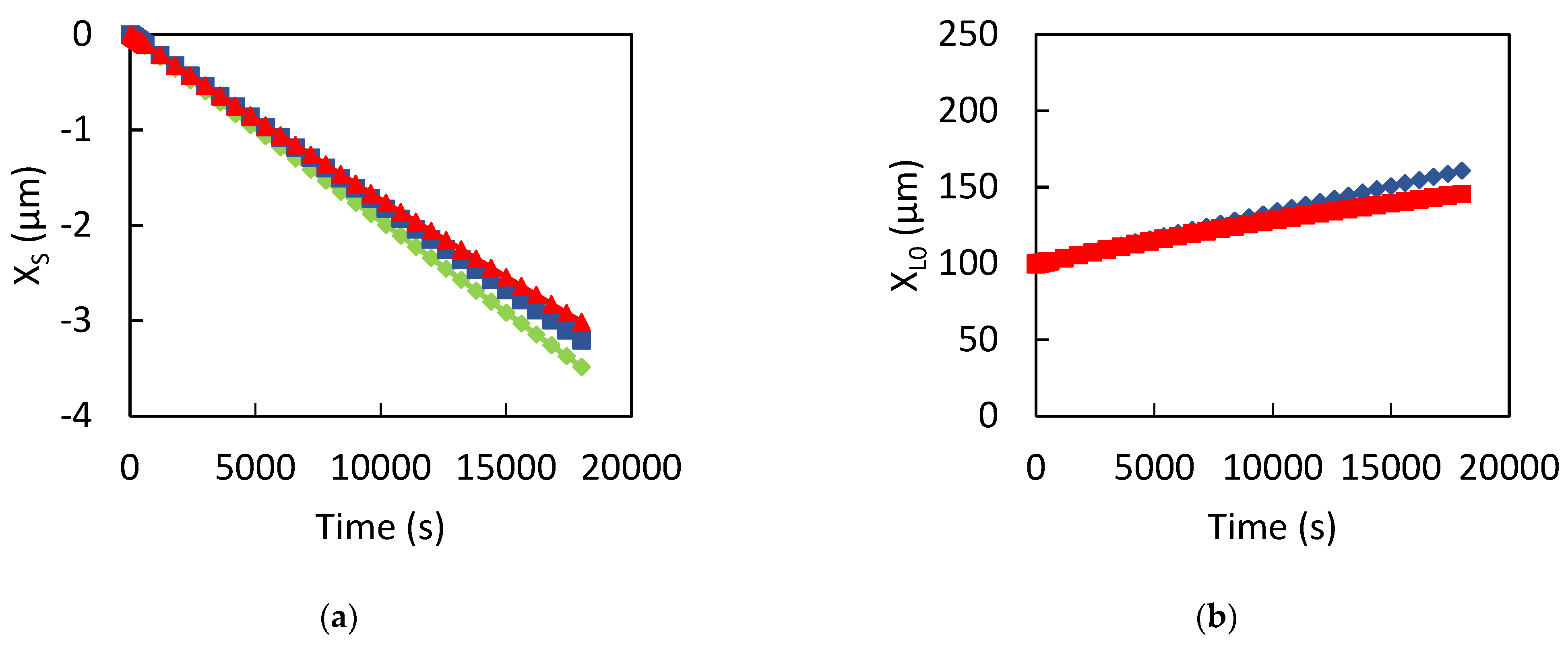
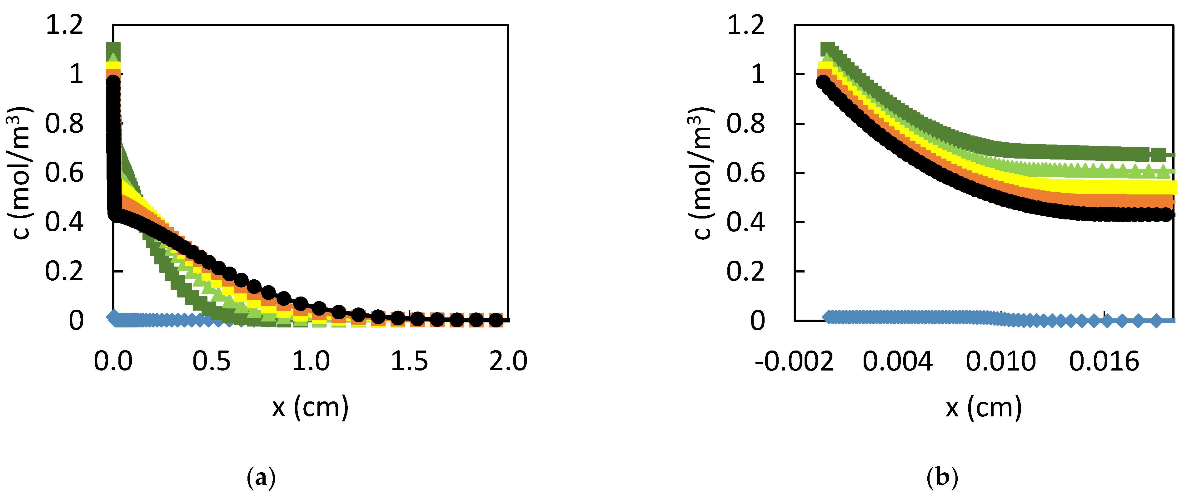
3.1. Dissolution of Lead

The first step is to study the dissolution of lead in a 1000 mol/m3 HCl. Only four species are taken into account: lead ions Pb2+, proton H+, dihydrogen H2, and chloride ions Cl. The input parameters and boundary conditions implemented are presented above. The simulation is carried out potentiostatically at the corrosion potential Ecor, over a time of 18,000 s, which corresponds to a duration of 5 h.
During the simulation, the potential is imposed at the electrode surface on the value of Ecor, which gives an anode current ia and a cathode current ic tending towards icor (Figure 5). The value of ic is negative in accordance with a cathodic current. During the first seconds, the current is null and then grows up. This is because the dissolution takes place only after few seconds and none at t0, giving the system time to balance itself.
Figure 6 shows the evolution of the concentration of the different ions within the electrolyte, x = 0 cm being the surface of the lead electrode xs with an electrolyte of L = 10 cm. The dissolution of lead creates ions of valence 2+, which explains the increase in the Pb2+ concentration in the electrolyte. The concentration profile is decreasing, and the area where the concentration is different from the initial concentration increases with time. After 18,000 s, Pb2+ ions are present 1 cm from the surface of the electrode. By comparing this value to the characteristic diffusion length δ defined as:
δ = D t
where D is the coefficient of Pb2+ ions of 9.39 × 10⁻¹⁰ m²·s−1 and t is the final time of 18,000 s, we may obtain a value of δ of 0.41 cm. This value clearly shows a process where the diffusion is not the only motor, but is also accompanied by the migration process (linked to the electric potential gradient).
In the cathodic process, protons are consumed and hydrogen is formed. The H+ concentration at the electrode surface decreases over time as the depleted area grows (Figure 6b). Its size after 18,000 s is greater than that of lead or hydrogen as their diffusion coefficient (Table 2). The profile of H2, considered as a species of zero charge in the solution, shows a similar appearance to that of lead. However, the enrichment is presented on a larger zone (Figure 6c). The electro-neutrality of the solution is established from the concentration of chloride ions, which is calculated according to Equation (7). The shape of the curve, presented in Figure 6d, exhibits an increase in the concentration of Cl to compensate the creation of cations near the surface of the electrode. Consequently, a depletion for larger values of x is present. There is no creation or loss of material, only a phenomenon of diffusion and migration.
The change in the position of the electrode surface as a function of time quantifies the loss of thickness of the specimen (Figure 7a, green curve). The slope of the line, equal to 1.944 × 10⁻⁴ µm/s, makes it possible to calculate the rate of dissolution of lead in 1000 mol/m3 HCl, which is equal to 6130.6 µm/yr (Table 2).
After 18,000 s, the corrosion of the lead electrode leads to a depletion (respectively, enrichment) over the large distance of the electrolyte. Taking the example of lead ions (Figure 6a), it can be seen that the concentration at xs has a value greater than the initial value, summing at around 40 mol/m3. Conversely, the chloride concentration is around 1022 mol/m3 (Figure 6d). The question arises of the future of these ions. Indeed, a solution can concentrate until its saturation, leading to the precipitation of solid species such as PbCl2. Using a value of the solubility product of Ksp = 10−4.81, and the law that relates the solubility s (mol/m3) to the solubility product:
K sp P b 2 + C l 2 c 0 3 = 4 s 3 c 0 3  
A solubility value of 15.7 mol/m3 would be required. The dissolution simulation points a greater value near the electrode. That means that the production of lead chloride PbCl2 seems to be possible.

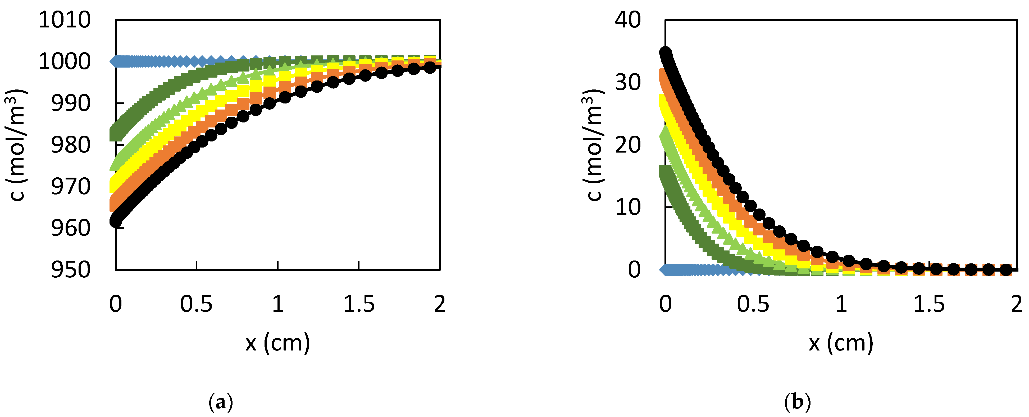
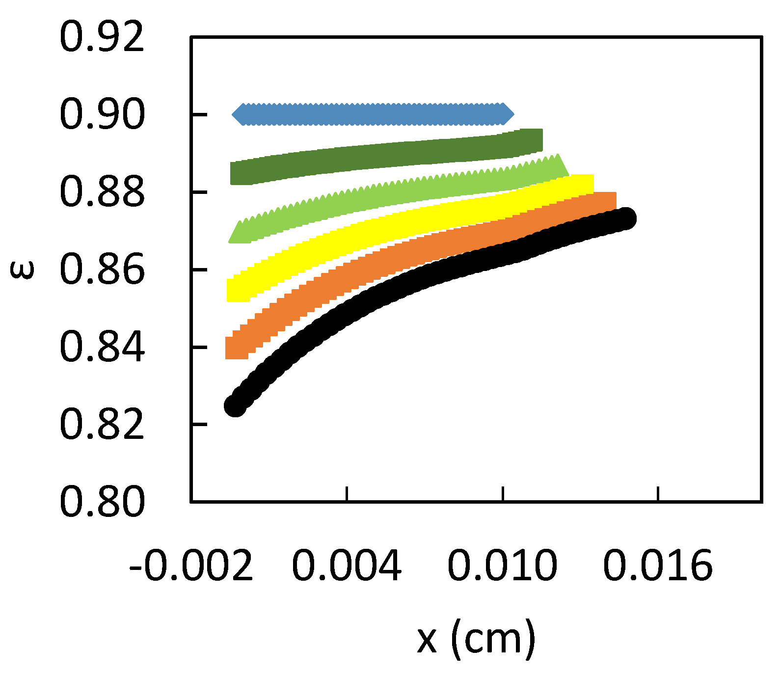
3.2. Influence of the CPL

To simulate this precipitation phenomenon, the possible growth of a CPL is taken into account. In the initial state, the thin layer measures L0 = 100 µm for an electrolyte of L = 10 cm. At t = 0 s, the CPL has a concentration of Pb2+ such that the saturation of the layer is equal to 1. The layer is therefore at equilibrium, which means a saturation SPbCl2 is at 1. The porosity cannot evolve and is fixed at 0.9. The idea is to study only the growth due to the interface’s movement.
The precipitation leads to a decrease of the Pb2+ ions in solution (Figure 8); with a maximum at 1.1 mol/m3 in the CPL The concentration increases during a first phase and then decreases. The CPL is completely saturated, which explains the wave of the profile whose height decreases with time. The whole layer is depleted in chloride ions (Figure 9) which clearly shows the consumption due to the PbCl2 formation. On the other hand, precipitation has no major influence on the cationic part (Figure 10); indeed, profiles of proton and H2 are similar in appearance to the one obtained in the previous part without CPL (Figure 6c,d), but we can see lower concentration values in agreement with the presence of the layer.
The curves in blue of Figure 7 present the evolution of the size of the CPL by plotting the position of the surface xs and of the interface L0 with xL0 as a function of time. The electrode surface follows the same evolution due to the dissolution. The presence of the corrosion product layer slows the dissolution with a rate of 5629.2 µm/yr. On the other hand, the size of PbCl2 increases, which leads to a movement of the position of L0 to bigger values with a position at xL0 = 150 µm after 18,000 s. The growth is linear, with an unrealistic growth rate greater than 100,000 µm/yr. This value is non-realistic and shows the fact that in real life, the corrosion product layer does not have a fixed porosity but can become denser over time.
To be more realistic, the variation of the porosity is added throughout the CPL layer according to the equation, with an initial value of 0.9. Like before, the layer grows at the surface of the lead electrode by dissolution and by precipitation of PbCl2 at x = L0. Initially at 100 µm, the layer has a thickness of more than 146 µm those that are smaller than the one obtained with a fixed porosity (Figure 7). This layer growth is accompanied by a densification of the layer as evidenced by the evolution of epsilon, which reflects the porosity. Initially at 0.9, close to the surface, the porosity reaches a value around 0.82, and around 0.88 at the surface of the corrosion product layer (Figure 11). The difference in values between the surface of the electrode and the layer of corrosion product is linked to the surface stress, which can only move by dissolution (Figure 7 and Table 2) when the interface L0 is free. However, the Figure 11 shows that the precipitation engine is more important at the surface of the electrode than at the interface CPL/electrolyte. This is linked to the place of creation of the ions (i.e., the electrode surface xs). It can also be noted by the difference in the value of the SST and Rp parameters (Figure 12). Rp as defined in Equation (24) is a kinetic indicator which translates the PbCl2 precipitation. Its value is lower at the CPL–electrolyte interface than at the surface of the electrode. Moreover, the evolution of the porosity also modifies the RP value as evinces Figure 12a, with the comparison of the case with fixed porosity and the one where porosity varies.
The Surface Scaling Tendency SST allows comparing the rate of vacuum creation by dissolution and the rate of precipitation:
SST = k p K s p S P b C l 2 1 i ε 2 F
The SST is always less than one, which shows that the dissolution rate is more important than the precipitation rate. Therefore, more Pb2+ is created than PbCl2 consumed. This is confirmed by the precipitation rate Rp, which is greater at the surface of the electrode than at the level of the surface of the layer of the corrosion product. The fact that the porosity is variable affects both the precipitation and the dissolution. Indeed, the dissolution kinetics are slower as evidenced by the Figure 7a and the precipitation by densification of the layer greater. This explains the difference in SST value between the case with fixed porosity and the case with variable porosity (Figure 12b).
The shape of the profiles does not change as well for the lead ions (Figure 13) as it does for the chlorides (Figure 14). On the other hand, a difference appears at the level of the concentration values; that is, with a Pb2+ concentration of 1 mol/m3, the layer is more depleted, showing the formation of PbCl2. This trend is not visible at the level of chlorides, the concentration of which is calculated from the other elements. Nevertheless, the growth of the porosity is materialized by a slowing down of the cathodic process, with a higher proton concentration whereas that of H2 is lower after 18,000 s (Figure 15). However, these variations are small with regard to the whole of the electrolyte as evidenced by the saturation, the appearance of which is similar between the fixed porosity case and the variable porosity one (Figure 16).

4. Discussion

This article presents the developmental progress of a numerical tool able to simulate the corrosion mechanism of lead exposed to an anaerobic solution of HCl. The code is developed under COMSOL Multiphysic. The choice of 1D development was made to simplify the handling of the tool and highlight trends.
To simulate the anodic and cathodic parts of the corrosion process, input data is needed. In this sense, the code was developed using data from the literature (Table 1).
The simulation of corrosion was approached by using an electrolyte of finite size L = 10 cm making it possible to reproduce a so-called “full bath” electrolyte. The purpose of this step is to simulate the general dissolution that affects lead when it is immersed in deaerated hydrochloric acid. After 18,000 s of immersion, a dissolution rate of about 6 mm/year is obtained. This value shows the reactivity of lead in HCl, but also the overestimation of the corrosion rate established from electrochemical data, a phenomenon well-known in the literature [39]. Nevertheless, the simulation objective of the dissolution is to obtain a reference state, which allows us to study the impact of the presence of a corrosion product layer.
The dissolution of the material leads to the formation of 2+ valence ions, which concentrate the electrolyte, particularly near the surface of the electrode. The value of the concentration of lead ions is higher than the solubility limit creating a saturation of the electrolyte, as is in agreement with the experimental results that show a tendency to passivation, as materialized by the precipitation of PbCl2 at the Pb surface [40,41].
The presence of this chloride product was taken into account by the implementation of a layer of porous corrosion product on the surface of the electrode, denoted CPL. SEM observations carried out during the corrosion process show a process of corrosion product formation into two steps. Initially islands of PbCl2 are created then grow until they form a compact and fissured layer. In this sense, a porous corrosion product layer was initially placed to simulate these islands [41].
If the porosity is constant and does not change over time, the layer grows in space. In contact with this layer, the dissolution of the lead decreases, with a kinetic value lower than that obtained in full bath. This leads to lower lead ion concentrations than those obtained without CPL. However, the concentration is higher than the initial CPL concentration of 0.015 mol/m3. This supersaturation of the CPL tends to show that over time, there are enough Pb2+ ions in the CPL to form PbCl2, and therefore to cause the porosity to evolve.
The implementation of the porosity variation shows a corrosion phenomenon of mixed growth where the layer has both an increasing thickness over time as well as a decreasing epsilon, which means an increase of porosity. This evolution is due to a densification of the layer. It is not homogeneous within the CPL. The layer is more compact on the surface of the electrode than in contact with the electrolyte, in agreement both with the location of the creation of Pb2+ and also with the observations of PbCl2 made electrochemically; therefore, there is a competition between surface growth and dissolution [42].
Nevertheless, this evolution of the layer is not sufficient to have a saturation lower than 1 near the surface of the electrode and in the CPL for short periods of time. Although a decrease in the concentration of lead ions is visible, lead is present up to 1 cm in the electrolyte after 18,000 s. This shows that over longer amounts of time, we can expect to have a thicker layer whose compactness is greater in accordance with the experimental results.
Currently, an intermediate stage with the appearance of the first PbCl2 germs has not been taken into account. Generally, the precipitation of the first crystal germ is based on the germination-growth theory [43,44]. Germination, also called nucleation [45], corresponds to the spontaneous formation of crystalline germs of a solid phase in a supersaturated solution. Nucleation plays a decisive role in the process of determining the crystal structure and size distribution of crystals. The nucleation phase is followed by the growth phase where the germ created during the nucleation phase will grow by progressive addition of atoms or molecules to its surface. When several germs have formed and have reached a certain size, a third phase called agglomeration takes place. With this decomposition appears the need to pose several hypotheses and the establishment of artificial criteria determining the passage from one to the other [46]. Experimentally, the growth and agglomeration phases of PbCl2 have been observed on the surface of lead in contact with a humid environment polluted by HCl [40,41]. Taking into account the creation of this layer is therefore a necessary step for the implementation of the global corrosion process.
Note that this is, however, not the only hypothesis to raise. Indeed, the environment of the study is anaerobic; therefore, oxygen is not taken into account. However, when lead is exposed to the liquid HCl acid, oxygen is a major element of the corrosion phenomenon that can lead to the formation of oxide such as PbO2 or complex as PbOCl [41,47,48]. Taking it into account is therefore a necessary step to obtain the most accurate model possible.

5. Conclusions

This article shows the first numerical progressions carried out to develop a tool capable of simulating the behaviour of lead exposed to HCl, a powerful acid. These developments, completed with COMSOL Multiphysics, were carried out in dimension 1 of space and by considering an anaerobic electrolyte. The digital development was carried out in several stages in order to study and validate each of them. We made the assumption of working at the corrosion potential in potentiostatics.
The results of the simulations show that:
  • When lead is immersed in HCl, it dissolves. This dissolution leads to saturation of the electrolyte with the consequent precipitation of corrosion product;
  • The PbCl2 corrosion product layer has an impact on the dissolution kinetics. Its development takes place by growth in space but also by densification, with an evolution of epsilon;
  • The PbCl2 layer is more compact near the surface of the electrode in accordance with the place of creation of the ions.
These results are in agreement, with the experimental results and make it possible to validate this first approach.
This study is only a first step, in that it must be supplemented by taking into account oxygen, an essential element of the corrosion phenomenon, and by a development in dimension.

Author Contributions

Writing–original draft, F.L. and M.M. All authors have read and agreed to the published version of the manuscript.

Funding

This research received no external funding.

Institutional Review Board Statement

Not applicable.

Informed Consent Statement

Not applicable.

Data Availability Statement

The data presented in this study are available on request from the corresponding author. The data are not publicly available due to partners.

Acknowledgments

The authors would like to thank Orano and EDF partners for financial support.

Conflicts of Interest

The authors declare no conflict of interest.

References

  1. Austin, S.; Glowacki, A. Hydrochloric Acid. In Ullmann’s Encyclopedia of Industrial Chemistry; Wiley: Hoboken, NJ, USA, 2000. [Google Scholar]
  2. Lecloux, A. Chemical, biological and physical constrains in catalytic reduction processes for purification of drinking water. Catal. Today 1999, 53, 23–34. [Google Scholar] [CrossRef]
  3. Bagchi, P.; Karpinski, P.H.; McIntire, G.L. Microprecipitation of Nanoparticulate Pharmaceutical Agents. U.S. Patent US5560932A, 1 October 1996. [Google Scholar]
  4. Karlsson, A.; Ejlertsson, J. Addition of HCl as a means to improve biogas production from protein-rich food industry waste. Biochem. Eng. J. 2012, 61, 43–48. [Google Scholar] [CrossRef]
  5. Kim, J.; McVittie, J.; Saraswat, K.; Nishi, Y.; Liu, S.; Tan, S. Germanium Surface Cleaning with Hydrochloric Acid. ECS Trans. 2006, 3, 1191–1196. [Google Scholar] [CrossRef]
  6. Sun, Y.; Liu, Z.; Sun, S.; Pianetta, P. The effectiveness of HCl and HF cleaning of Si0.85Ge0.15 surface. J. Vac. Sci. Technol. A Vac. Surf. Film. 2008, 26, 1248–1250. [Google Scholar] [CrossRef]
  7. Tomaszewska, M.; Gryta, M.; Morawski, A.W. Recovery of hydrochloric acid from metal pickling solutions by membrane distillation. Sep. Purif. Technol. 2001, 22-23, 591–600. [Google Scholar] [CrossRef]
  8. Li, L.-F.; Caenen, P.; Celis, J.-P. Effect of hydrochloric acid on pickling of hot-rolled 304 stainless steel in iron chloride-based electrolytes. Corros. Sci. 2008, 50, 804–810. [Google Scholar] [CrossRef]
  9. Lin, H.-W.; Cejudo-Marín, R.; Jeremiasse, A.W.; Rabaey, K.; Yuan, Z.; Pikaar, I. Direct anodic hydrochloric acid and cathodic caustic production during water electrolysis. Sci. Rep. 2016, 6, 20494. [Google Scholar] [CrossRef]
  10. Subramanian, K. Lead-Free Electronic Solders: A Special Issue of the Journal of Materials Science: Materials in Electronics; Springer: Berlin/Heidelberg, Germany, 2007. [Google Scholar]
  11. Lim, S.-R.; Schoenung, J.M. Human health and ecological toxicity potentials due to heavy metal content in waste electronic devices with flat panel displays. J. Hazard. Mater. 2010, 177, 251–259. [Google Scholar] [CrossRef]
  12. World Health Organization. Toolkit for Establishing Laws to Eliminate Lead in Paint; World Health Organization: Geneva, Switzerland, 2021. [Google Scholar]
  13. Baba, A.A.; Adekola, F.; Ghosh, M.K.; Salubi, Y.A.; Oyedotun, M.O.; Rout, P.O.; Sheik, A.R.; Pradhan, S.R. Leaching of Lead from Spent Motorcycle Battery in Hydrochloric Acid. Part I: Dissolution kinetics. Acta Metall. Slovaca 2010, 16, 194–204. [Google Scholar]
  14. El Wanees, S.A.; El Aal, E.A. N-Phenylcinnamimide and some of its derivatives as inhibitors for corrosion of lead in HCl solutions. Corros. Sci. 2010, 52, 338–344. [Google Scholar] [CrossRef]
  15. El Rehim, S.A.; El-Halim, A.A.; Foad, E. Potentiodynamic and cyclic voltammetric behaviour of the lead electrode in HCl solutions. Surf. Technol. 1983, 18, 313–325. [Google Scholar] [CrossRef]
  16. Aaal, E.E.A.E.; El Wanees, S.A. Kinetics of anodic behaviour of Pb in HCl solutions. Corros. Sci. 2009, 51, 458–462. [Google Scholar] [CrossRef]
  17. Barradas, R.G.; Belinko, K.; Ghibaudi, E. Rotating Ring-disc Electrode Studies of Lead in HCl and NaCl Solutions. Can. J. Chem. 1975, 53, 407–413. [Google Scholar] [CrossRef]
  18. Barradas, R.; Fletcher, S.; Porte, J. The anodic behaviour of lead amalgam electrodes in HCl solution. J. Electroanal. Chem. Interfacial Electrochem. 1977, 80, 295–304. [Google Scholar] [CrossRef]
  19. Barradas, R.; Belinko, K.; Shoesmith, W. Study of surface effects in the formation of lead chloride on lead electrodes in aqueous HCl by electrochemical methods and scanning electron microscopy. Electrochim. Acta 1976, 21, 357–365. [Google Scholar] [CrossRef]
  20. Ambrose, J.; Barradas, R.; Belinko, K.; Shoesmith, D. Reactions at the lead electrode/hydrochloric acid interface. J. Colloid Interface Sci. 1974, 47, 441–454. [Google Scholar] [CrossRef]
  21. Azizi, A.; Ghasemi, S.M.S. A comparative analysis of the dissolution kinetics of lead from low grade oxide ores in HCl, H2SO4, HNO3 and citric acid solutions. Met. Res. Technol. 2017, 114, 406. [Google Scholar] [CrossRef]
  22. Baba, A.; Sheik, A.R.; Olawale, K.I.; Young, T.; Ghosh, M.K.; Folahan, A.A. Kinetic analysis of total Lead from spent Car battery by hydrochloric acid leaching. J. Iran. Chem. Res. 2011, 4, 291–300. [Google Scholar]
  23. Barradas, R.; Fletcher, S. Temperature effects in the electrochemical behaviour of cycled lead electrodes in HCl solutions. Electrochim. Acta 1977, 22, 237–242. [Google Scholar] [CrossRef]
  24. Van Herck, P.; Van der Bruggen, B.; Vogels, G.; Vandecasteele, C. Application of computer modelling to predict the leaching behaviour of heavy metals from MSWI fly ash and comparison with a sequential extraction method. Waste Manag. 2000, 20, 203–210. [Google Scholar] [CrossRef]
  25. Rooney, C.P.; McLaren, R.G.; Condron, L.M. Control of lead solubility in soil contaminated with lead shot: Effect of soil pH. Environ. Pollut. 2007, 149, 149–157. [Google Scholar] [CrossRef] [PubMed]
  26. Inamuddin, A.M.I.; Luqman, M.; Altalhi, T. Sustainable Corrosion Inhibitors; Materials Research Forum: Millersville, PA, USA, 2021; Volume 107. [Google Scholar]
  27. Liu, C.; Kelly, R.G. A Review of the Application of Finite Element Method (FEM) to Localized Corrosion Modeling. Corrosion 2019, 75, 1285–1299. [Google Scholar] [CrossRef] [Green Version]
  28. Simillion, H.; Dolgikh, O.; Terryn, H.; Deconinck, J. Atmospheric corrosion modeling. Corros. Rev. 2014, 32, 73–100. [Google Scholar] [CrossRef]
  29. Tricoit, S. Modeling and Numerical Simulation of the Propagation of Pitting Corrosion of Iron in Chlorinated Medium: Contribution to the Evaluation of the Durability of Carbon Steels in Geological Storage Conditions. Ph.D. Thesis, Université de Bourgogne, UFR Sciences et Techniques, Laboratoire Interdisciplinaire Carnot de Bourgogne-LICB (France), Dijon, France, 2012. [Google Scholar]
  30. Radouani, R.; Echcharqy, Y.; Essahli, M. Numerical Simulation of Galvanic Corrosion between Carbon Steel and Low Alloy Steel in a Bolted Joint. Int. J. Corros. 2017, 2017, 6174904. [Google Scholar] [CrossRef]
  31. Trinh, D.; Ducharme, P.D.; Tefashe, U.M.; Kish, J.R.; Mauzeroll, J. Influence of Edge Effects on Local Corrosion Rate of Magnesium Alloy/Mild Steel Galvanic Couple. Anal. Chem. 2012, 84, 9899–9906. [Google Scholar] [CrossRef]
  32. Landolt, D. Corrosion et Chimie de Surfaces des Métaux; Traité des Matériaux, Collection; Romandes, P.P.E.U., Ed.; EPFL Press: Lousanne, Switzerland, 1997. [Google Scholar]
  33. Mohamed-Saïd, M. Modélisation du Rôle des Produits de Corrosion sur L’évolution de la Vitesse de Corrosion des Aciers au Carbone en Milieu Désaéré et Carbonaté: Modelling of the Role of Corrosion Products on the Evolution of the Corrosion Rate of Carbon Steel in Deaerated and Carbonated Media. Ph.D. Thesis, University de Bourgogne Franche-Comté, Dijon, France, 2018. [Google Scholar]
  34. Mohamed-Said, M.; Vuillemin, B.; Oltra, R.; Marion, A.; Trenty, L.; Crusset, D. Predictive modelling of the corrosion rate of carbon steel focusing on the effect of the precipitation of corrosion products. Corros. Eng. Sci. Technol. 2017, 52, 178–185. [Google Scholar] [CrossRef]
  35. Mohamed-Said, M.; Vuillemin, B.; Oltra, R.; Trenty, L.; Crusset, D. One-Dimensional Porous Electrode Model for Predicting the Corrosion Rate under a Conductive Corrosion Product Layer. J. Electrochem. Soc. 2017, 164, E3372. [Google Scholar] [CrossRef]
  36. El-Lateef, H.M.A.; El-Sayed, A.-R.; Mohran, H.S.; Shilkamy, H.A.S. Corrosion inhibition and adsorption behavior of phytic acid on Pb and Pb–In alloy surfaces in acidic chloride solution. Int. J. Ind. Chem. 2019, 10, 31–47. [Google Scholar] [CrossRef]
  37. Sato, H.; Yui, M.; Yoshikawa, H. Ionic Diffusion Coefficients of Cs+, Pb2+, Sm3+, Ni2+, SeO2−4 and TcO4 in Free Water Determined from Conductivity Measurements. J. Nucl. Sci. Technol. 1996, 33, 950–955. [Google Scholar] [CrossRef]
  38. Lothenbach, B.; Ochs, M.; Wanner, H.; Yui, M. Thermodynamic Data for the Speciation and Solubility of Pd, Pb, Sn, Sb, Nb and Bi in Aqueous Solution; Japan Nuclear Cycle Development Institute: Tokai, Japan, 1999. [Google Scholar]
  39. Poorqasemi, E.; Abootalebi, O.; Peikari, M.; Haqdar, F. Investigating accuracy of the Tafel extrapolation method in HCl solutions. Corros. Sci. 2009, 51, 1043–1054. [Google Scholar] [CrossRef]
  40. Lequien, F.; Moine, G. Corrosion of a 75Sn/25Pb coating on a low carbon steel in a gaseous environment polluted with HCl: Mechanism. Mater. Corros. 2018, 69, 1422–1430. [Google Scholar] [CrossRef]
  41. Lequien, F.; Moine, G.; Lequien, A.; Neff, D. The corrosion mechanism initiation of a 75Sn–25Pb coating on a low-carbon steel sample in HCl environments. Mater. Corros. 2021, 72, 1488–1505. [Google Scholar] [CrossRef]
  42. Barradas, R.G.; Belinko, K.; Ambrose, J. Electrochemical Behavior of the Lead Electrode in HCl and NaCl Aqueous Electrolytes. Can. J. Chem. 1975, 53, 389–406. [Google Scholar] [CrossRef]
  43. Poupelloz, E. Etude des Processus de Germination-Croissance de L’ettringite, Seule ou dans un Système Aluminate Tricalcique/Sulfate de Calcium. Ph.D. Thesis, Université Bourgogne Franche Comté, Dijon, France, 2019. [Google Scholar]
  44. Cormier, L. La Théorie Classique de la Nucléation; Université Pierre et Marie Curie: Paris, France, 2013. [Google Scholar]
  45. De Yoreo, J.J.; Vekilov, P.G. Principles of Crystal Nucleation and Growth. Rev. Mineral. Geochem. 2003, 54, 57–94. [Google Scholar] [CrossRef]
  46. Acevedo Reyes, D. Evolution de L’état de Précipitation au Cours de L’austénitisation D’aciers Microalliés au Vanadium et au Niobium. Ph.D. Thesis, INSA de Lyon, Lyon, France, 2007. [Google Scholar]
  47. Wei, L.-Y.; Yang, Y.-W.; Lee, J.-F. Lead speciation in 0.1 N HCl-extracted residue of analog of Pb-contaminated soil. J. Electron Spectrosc. Relat. Phenom. 2005, 144, 299–301. [Google Scholar] [CrossRef]
  48. Mohammadi, M.; Alfantazi, A. Anodic behavior and corrosion resistance of the Pb-MnO2 composite anodes for metal electrowinning. J. Electrochem. Soc. 2013, 160, C253. [Google Scholar] [CrossRef]
Figure 1. Schematic representation of a lead electrode exposed to a deaered HCl electrolyte. Initially, the thickness of the electrolyte is L and the surface S of lead is at x = 0.
Coatings 12 01291 g001
Figure 2. Schematic representation of the dissolution of the lead test tube immersed in a deaerated HCl solution. (a) at t0 and (b) at t.
Coatings 12 01291 g002
Figure 3. Schematic representation of the movement of the CPL corrosion product layer (domain (2)) of size x = L0. (a) At t0, (b) evolution during dissolution of the lead electrode and (c) precipitation of PbCl2.
Coatings 12 01291 g003
Figure 4. Schematic representation of the evolution of the CPL by variation of the porosity over time. The points S, L0 and L are fixed. (a) ε at t0 and (b) ε at t.
Coatings 12 01291 g004
Figure 5. Evolution of (a) the potential and (b) the current density (black) anodic and (red) cathodic part at the surface of the electrode x = S.
Coatings 12 01291 g005
Figure 6. Evolution of the ion concentration in an electrolyte of 1000 mol/m3 HCl and of size L = 10 cm with only the first 2 cm are presented for six times t = 0 s (light blue), 3600 s (dark green) 7200 s (green), 10,800 s (yellow), 14,400 s (orange), and 18,000 s (black). (a) Pb2+ ions, (b) H+ ions, (c) H2 and (d) Cl ions.
Coatings 12 01291 g006
Figure 7. Evolution of (a) the position of the electrode surface xs (µm) and (b) position of CPL electrolyte interface xL0 (µm). Simulation with only dissolution (green), a fixed porosity (blue), and a variable porosity (red).
Coatings 12 01291 g007
Figure 8. Evolution of the lead ion concentration in an electrolyte of 1000 mol/m3 HCl and of size L = 10 cm with an initial CPL of 100 µm and a fixed porosity of 0.9 (a) The first 2 cm and (b) the first 200 µm of the electrolyte are presented for different times t = 0 (light blue), 3600 (dark green) 7200s (green), 10,800 s (yellow), 14,400 s (orange), and 18,000 s (black).
Coatings 12 01291 g008
Figure 9. Evolution of the chloride ion concentration in an electrolyte of 1000 mol/m3 HCl and of size L = 10 cm with an initial CPL of 100 µm and a fixed porosity of 0.9 (a) the first 2 cm and (b) the first 200 µm of the electrolyte are presented for different times t = 0 s (light blue), 3600 s (dark green) 7200 s (green), 10,800 s (yellow), 14,400 s (orange), and 18,000 s (black).
Coatings 12 01291 g009
Figure 10. Evolution of (a) the protons and (b) H2 concentration in an electrolyte of 1000 mol/m3 HCl and of size L = 10 cm with an initial CPL of 100 µm and a fixed porosity of 0.9. The first 2 cm of the electrolyte are presented for different times t = 0 s (light blue), 3600 s (dark green) 7200 s (green), 10,800 s (yellow), 14,400 s (orange), and 18,000 s (black).
Coatings 12 01291 g010
Figure 11. Evolution of the porosity of the CPL in an electrolyte of 1000 mol/m3 HCl of a size L = 10 cm with an initial CPL of 100 µm as a function of time (s) presented for different times t = 0 s (light blue), 3600 s (dark green) 7200 s (green), 10,800 s (yellow), 14,400 s (orange), and 18,000 s (black).
Coatings 12 01291 g011
Figure 12. Evolution of (a) Rp and SST(b) as a function of time (s) for ( )   L 0   and   ( ) S with (blue) the fixed porosity case and (red) the variable porosity case.
Coatings 12 01291 g012
Figure 13. Evolution of the lead ion concentration in an electrolyte of 1000 mol/m3 HCl and of size L = 10 cm with an initial CPL of 100 µm and a variable porosity (a) the first 2 cm and (b) the first 200 µm of the electrolyte are presented for different times t = 0 (light blue), 3600 (dark green) 7200s (green), 10,800 s (yellow), 14,400 s (orange), and 18,000 s (black).
Coatings 12 01291 g013
Figure 14. Evolution of the chloride ion concentration in an electrolyte of 1000 mol/m3 HCl and of size L = 10 cm with an initial CPL of 100 µm and a variable porosity (a) the first 2 cm and (b) the first 200 µm of the electrolyte are presented for different times t = 0 (light blue), 3600 (dark green) 7200 s (green), 10,800 s (yellow), 14,400 s (orange), and 18,000 s (black).
Coatings 12 01291 g014
Figure 15. Evolution of (a) the protons and (b) H2 concentration in an electrolyte of 1000 mol/m3 HCl and of size L = 10 cm with an initial CPL of 100 µm and a fixed porosity of 0.9. The first 2 cm of the electrolyte are presented for different times t = 0 s (light blue), 3600 s (dark green) 7200 s (green), 10,800 s (yellow), 14,400 s (orange), and 18,000 s (black).
Coatings 12 01291 g015
Figure 16. Evolution of SPbCl2 (a) on the first 2 cm and (b) on the first 200 µm of the electrolyte, for (blue) the fixed porosity case and (red) the variable porosity case.
Coatings 12 01291 g016
Table 1. Value of some parameters and units.
ParametersDescriptionValue/UnitRef.
EcorCorrosion potential−0.554 V[36]
Eeq_PbReference potential for Pb2+/Pb−0.688 V[14]
Eeq_HReference potential for H+/H2−0.248 V
i0_PbApparent exchange current density of Pb2+1.05 × 10⁻⁴ mA/cm²[36]
i0_HApparent exchange current density of H+11.82 × 10⁻⁴ mA/cm²[36]
baAnodic Tafel parameter0.041 V/dec[36]
bcCathodic Tafel parameter−0.138 V/dec[36]
αTransfer charge coefficient0.4
DPb2+Diffusion coefficient of Pb2+9.39 × 10⁻¹⁰ m²/s[37]
DH+Diffusion coefficient of H+9.30 × 10⁻⁹ m²/s[33]
DH2Diffusion coefficient of H21.00 × 10−9 m²/s[33]
DCl-Diffusion coefficient of Cl2.03 × 10−9 m²/s[33]
c0Initial concentration1000 mol/m3
cH2_0Initial concentration10−6 mol/m3
cCl_0Initial concentration1000 mol/m3[36]
cH_0Initial concentration1000 mol/m3[36]
KspSolubility product10−4.81[38]
kpPrecipitation kinetic constant of PbCl210−4 mol/(m²·s)
ρPbCl2PbCl2 density5.85 g/m3
MPbCl2Molar PbCl2 weight278.10 g/mol
ρPbPb density11.35 g/m3
MPbMolar Pb weight207.20 g/mol
RpSize of a crystal and is fixed10−7 m[33].
Table 2. Extrapolation of the curves in Figure 7a to determine the dissolution kinetics of the lead surface immersed in 1000 mol/m3 of HCl for 18,000 s.
SchemeSlope (µm/s)Corrosion Rate (µm/yr)
Dissolution1.944 × 10−46130.6
Fixe epsilon1.785 × 10−45629.2
Variable epsilon1.696 × 10−45348.5
Publisher’s Note: MDPI stays neutral with regard to jurisdictional claims in published maps and institutional affiliations.

