Abstract
This study focusses on investigating the effect of flow orientation on global and local two-phase flow parameters under two-phase flow conditions. Flow visualization, pressure measurement, and conductivity probe measurements are performed in a test facility made of 50.8 mm inner diameter acrylic pipes with flow visualization, pressure measurement, and conductivity probe measurement. Characteristics of flow regimes and interfacial structures, and frictional pressure drop prediction in the vertical upward and vertical downward two-phase flows are compared and analyzed. The results show that unique coring phenomenon and slug bubbles with off-centered noses appear in the vertical downward flow. The flow regime transition boundaries shift to the lower gas superficial velocities in the vertical downward flow compared to that in the vertical upward flow. Furthermore, the distribution and one-dimensional transport of the void fraction, interfacial area concentration, bubble velocity, bubble Sauter-mean diameter, and bubble frequency are acquired and compared to study the effect of flow orientation on interfacial structures. The interfacial structure and its development are found to be mainly affected by the lift force and the turbulence related bubble interactions. The frictional pressure drop is acquired and modeled by the Lockhart–Martinelli correlation. The frictional pressure drop is found to be larger in the vertical upward flow than that in the vertical downward flow. The recommended C value for both vertical upward and vertical downward flows are proposed.
1. Introduction
Vertical two-phase flows exist widely in engineering applications such as heat exchangers, oil transport pipelines, chemical processing plants, and nuclear reactors. Different from single-phase flow, characteristics of two-phase flow shows dependence on flow orientation due to the buoyancy effect. For example, stratified and wave flow regimes exist in horizontal two-phase flow but are not observed in vertical two-phase flow [1]. As a result, the flow regimes that exist in vertical and horizontal orientations are different. The dissipation of the elbow effect on two-phase flow downstream of the vertical upward and vertical downward elbows are also found to be different [2]. For vertical two-phase flows, coring of bubbles is observed in the downward two-phase flow but not observed in the upward flow [3,4,5]. The determination of the correct flow regime is the basis for accurate selecting of the regime-based empirical correlations, and the interfacial structure directly affect the interfacial mass, moment, and energy transfer. Therefore, it is necessary to investigate the effect of flow orientation on flow regime, interfacial structure, pressure drop, and other two-phase parameters.
For two-phase flow in vertical orientations, numerous studies have been performed to qualitatively model the flow in terms of flow regime classification and flow regime map development. A widely accepted flow regime map has been developed for vertical upward orientation, such as the Taitel and Dukler [6] and the Mishima and Ishii [7] flow regime maps. For vertical downward two-phase flow, Oshinowo and Charles [3], Barnea et al. [8], Usui and Sato [4], and Jiang and Rezkallah [9] all developed flow regime maps for vertical downward two-phase flow. However, no consensus has been reached on a universal downward flow regime map yet. This may be caused by the fact that downward two-phase flow may be more sensitive to channel shape and dimension, the inlet condition, and the historic effects [10]. Recently, Kazi et al. [11] experimentally studied the vertical upward and downward flows with a U-Bend inlet; the flow regime transitional boundaries for vertical upward flow agreed well with the Mishima and Ishii [7] map, but a worse agreement was achieved for the vertical downward flow.
The flow regime reflects the macroscopic characteristics of the two-phase flow; it is actually determined by the microscopic interfacial structure of the flow. The interfacial structure is described by parameters such as the interface shape, surface area density, and interfacial velocity between the gas and liquid phases. The momentum exchange between phases is through the work done by the interfacial shear stress on the interface, and the mass and energy exchange also need to pass the interfaces. For the vertical upward flow, studies by Serizawa et al. [12], Liu and Bankoff [13] and Wang et al. [14] show that the void fraction distribution is pretty uniform across the pipe cross-section with peaks near the wall in bubbly flow, and it changes to center-peaked distribution in slug flow. For vertical downward two-phase flow, Ishii et al. [15] and Hibiki et al. [16,17] studied the local interfacial structure and observed unique core-peaked void fraction distribution. With the area-averaged void fraction data, Kim et al. [18] shows that the drift flux model in downward flow is also different from that in upward flow.
For accurate prediction of the transient two-phase flow phenomena in reactor systems or other thermal systems, the two-fluid model is widely used in the system analysis codes [15]. Development of the closure relationships for interfacial transfer appear in the governing equations and requires understanding of the interfacial structures and interfacial area transport. Kim [19] and Sun et al. [20] studied the one-dimensional development of the interfacial structures in the vertical downward two-phase flow; Goda et al. [21], Hibiki et al. [22], and Kim et al. [18] characterized the evaluation of the one-dimensional interfacial structures in the downward two-phase flow.
Accurately predicting the pressure drop in two-phase flow systems is important as it affects the evaluation of two-phase flow parameters and the driving pump head. The two-phase pressure drop due to gravitation and acceleration can be estimated with velocity and void fraction information. The estimation of two-phase frictional pressure drops, however, relies on empirical correlations. Existing empirical correlations for two-phase frictional pressure drop prediction include the homogeneous flow model [23], separated flow model, and others. The Lockhart–Martinelli correlation [24] is one of the widely used separated flow models. The correlation contains a coefficient C, which needs to be determined for different flow structures.
Efforts have been performed to quantitatively compare the difference between vertical upward and vertical downward flows. Bhagwat and Ghajar [25] studied the difference flow regimes they obtained in vertical downward flow to the vertical upward ones from literature. Since the pipe diameter (12.7 mm) and experimental setup they used is different from those in literature, the comparison may introduce inaccuracy. Wang et al. [14] measured void fraction profile with a single-sensor probe showing that a distinct peak exists near the wall in upward flow but a “coring” peak appears in downward flow. Jiang et al. [9,26] used a single beam gamma densitometer to measure the void fraction values under different flow conditions in the upward and downward two-phase flows. They found that the void fraction in downward flow is usually higher than that in the upward flow and developed different correlations for void fraction prediction in different orientations. Unfortunately, only cross-sectional averaged void fraction data are provided due to the average measurement technique, and no other interfacial structure parameters information is discussed. Tian et al. [27] compared detailed interfacial structures measured with a four-sensor optical probe in upward and downward flows. However, measurements were performed at the 22 pipe diameter location, where the flow was suspected to be undeveloped.
Effects of flow orientations on flow regimes in non-usual channel dimension and channel geometry have also been investigated recently. Zeguai et al. [28] studied the orientation effects on two-phase flow regime evolution in a 3-mm diameter mini tube. They concluded the flow regime transitional boundaries are similar for upward and horizonal two-phase flow, but different in the downward two-phase flow. Abdulkadir et al. [29] performed vertical upward and downward two-phase flow in a 127 mm inner diameter pipe. Churn and annular flows were observed in upward flow, but only annular flow was observed in downward flow. Chalgeri and Jeong [30] studied the two-phase flow regimes in a narrow rectangular channel, and found the transition lines for bubbly to slug and slug to churn flowing in a vertical downward flow shift to the right of the transition lines observed in the vertical upward flow.
The authors have performed detailed experimental study on the effects of three types of inlets on vertical downward two-phase flow, i.e., injector without a flow straightener (Type A), injector with a flow straightener (Type B), and a 90° vertical elbow (Type C) [31]. Flow regime, interfacial structure, and frictional pressure drop were compared among the three types of inlets, which serves a good basis for investigation of the flow orientation effect. By acquiring new data in the vertical upward flow and comparing them to the published vertical downward flow data, the effect of flow orientation on two-phase flow can be investigated.
Many investigations have been performed to study the upward and downward two-phase flows. However, comparing experimental data acquired from different test facilities may encounter inconsistency, since two-phase flow is sensitive to the inlet conditions and geometric parameters. Further, due to lacking local interfacial data, detailed comparison of the microscopic and macroscopic interfacial structures between the vertical upward and vertical downward flows are rare. Therefore, the different interfacial and hydraulic characteristics between the upward and downward two-phase flows are not clear.
The present study aims to investigate the effect of flow orientation on two-phase flow by comparing the similarities and differences of vertical upward and vertical downward the two-phase flows. The objectives include the following: (1) analyze and compare the macroscopic characteristics of the vertical upward and vertical downward two-phase flow, including characteristics of flow regime and flow regime map, (2) analyze and compare evaluation of the local interfacial structure in different flow orientation, and (3) compare the two-phase frictional pressure drop in different flow orientations and establish the prediction model based on the Lockhart–Martinelli correlation.
2. Experimental Facility and Test Conditions
2.1. Test Facility and Instrumentation
Figure 1 shows the schematics of the test facility used to perform the two-phase flow experiments. The test facility is built up with acrylics pipes of vertical and horizontal orientations. The inner diameter (D) of the acrylic pipes is 50.8 mm. The test loop was designed to be capable of performing air–water two-phase flow in both vertical upward and vertical downward flow directions by switching the controlling valves, as indicated by the red and blue arrows in the figure. The water is stored in a plastic tank and pumped by a centrifugal pump; the air is stored in a stainless-steel tank and pressurized by a compressor. In both flow directions, two-phase flow is established by mixing the deionized water and compressed air in a sparger. The two-phase mixture flows either upward or downward, then reaches the separator, where air and water are separated by gravity. Air is released to atmosphere and the water flows back to the tank.
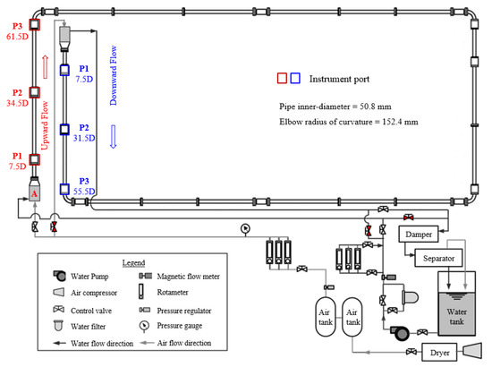
Figure 1.
Schematic diagram of the test facility.
The lengths of the vertical upward and vertical downward test sections are about 3.2 m and 2.9 m, respectively, yielding development lengths of 63D and 57D. It is built by connecting acrylic pipe section of different lengths and three instrumentation ports. Figure 2a shows the instrumentation port used for setup of measurement equipment, including the mount conductivity probe for two-phase parameter measurement, and is used to connect the pressure process line for the pressure transducer. All four sides of the instrumentation ports are shaved flat to minimize the optical distortion due to refraction during flow visualization experiments.
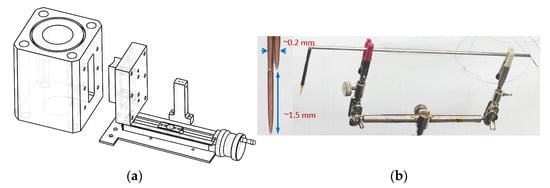
Figure 2.
(a) Instrumentation port for pressure and probe measurement and flow visualization, (b) Four-sensor conductivity probe.
In terms of the measurements, volumetric flow rates of air and water are monitored and set by the gas rotameter and electromagnetic flowmeter, respectively. Then, the volumetric flow rates are converted to the superficial velocities. The measurement uncertainties of the gas rotameter magnetic flowmeter are ±3% and ±5% of the measurement range, respectively. The pressure at each measurement port is measured by a differential pressure transducer. The measurement ranges of the transducer are varied to 0.75 kPa, 5 kPa, and 50 kPa at different flow conditions, which leads to corresponding measurement uncertainties of ±0.5%, ±0.1%, and ±0.1%, respectively. The minimized four-sensor conductivity probe [32], as shown in Figure 2b, is used to measure the local time-averaged interfacial parameters. For the flow visualization, a high-speed camera is used to capture the typical flow regimes. The measurement resolution is set to 512 × 512 pixels. The frame rate is set to 2000 to 4000 fps with a shutter speed of 1/10,000 s during the measurements.
2.2. Test Condition and Measurement Method
To compare the characteristics of the two-phase flow in different flow directions, conductivity probe measurements are performed at 7.5D, 34.5D, and 61.5D for three flow conditions for the vertical upward flow directions, as shown in Table 1. For the vertical downward flow, the published data by the authors [31] together with additional new data acquired are used to perform the comparison. Measurements were performed at 7.5D, 31.5D, and 55.5D for four flow conditions, as shown in Table 2. The flow conditions in tables are specified by the liquid superficial velocity (jf), and gas superficial velocity (jg), as indicated by Equations (1) and (2). As can be seen from Table 1 and Table 2, Run 2 and Run 3 in the vertical upward experiments have similar jf and jg,loc with Run 4 and Run 5 in the vertical downward experiments at the last measurement port, such that results of these flow conditions can be compared to study the effects of the orientation on two-phase flow.
where, Qf is the volumetric flow rate of water, Qg,loc is the volumetric flow rate of air evaluated at the pressure of last measurement port, i.e., 61.5D and 55.5D for the upward and downward flow, respectively. Qg,atm is the equivalent volumetric flow rate of air the at atmospheric pressure. Patm and Ploc are the atmospheric pressure and the gauge pressure at the last measurement port.

Table 1.
Test conditions vertical upward two-phase flow.
Table 2.
Test conditions vertical downward two-phase flow.
Since the interfacial structures of the two-phase flow can be assumed to be axisymmetric in the vertical directions, the variation of interfacial parameters measured along different pipe diameters are the same, such that probe measurements are performed along one diameter of the pipe at 15 radial positions, i.e., (r/R) = 0, ±0.2, ±0.4, ±0.5, ±0.6, ±0.7, ±0.8, and ±0.9, as shown in Figure 3. Here, r and R are the radial coordinate and radius of the pipe. To accurately position the measurement location, a conductivity probe is mounted on a linear position unit and traversed at different r/R. At each r/R location, conductivity probe signals are acquired by a data acquisition system for 30 s to 60 s with a sampling data acquisition frequency of 50 kHz. At least 2000 effective bubbles are acquired to get a statistically error of ±7% for conductivity probe measurements [33]. The acquired conductivity probe signals are processed by a data processing code to obtain the local time-averaged two-phase flow parameters, including the void fraction (α), the bubble frequency (fb), the bubble velocity (vg), and interfacial area concentration (ai).
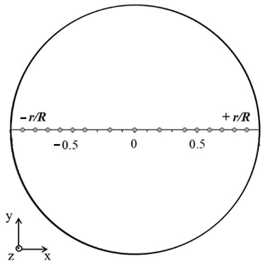
Figure 3.
Measurement mesh and coordinate systems for the conductivity probe.
2.3. Benchmark of the Probe Measurement
To assess the reliability of the conductivity probe measurement, the volumetric gas flow rates <αvg> calculated from the probe measurements are compared with the superficial velocities <jg>z calculated from the gas rotameters reading and the local pressure measurements. Here, the brackets denote the area-average operator. This evaluation compares the local and global measurement techniques for obtaining the volumetric gas flow rate at each measurement location. As demonstrated by Figure 4, the measurements for Runs 1–3 in the vertical upward flow agree well with two methods, but <αvg> underestimates <jg>z for Runs 4–7 in vertical downward flow. This is because when changing from Run 4 to Run 7, the bubble size increases as the gas phase flow rate increases. The accuracy of the conductivity probe measurements decreases as the flow approaches slug flow. Overall, an average absolute difference of 13.13% is considered acceptable in view of the accuracies of the conductivity probe, pressure transducer, back pressure dial gauge, and gas rotameters.
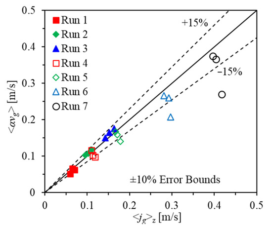
Figure 4.
Benchmark of the conductivity probe measurements.
3. Results and Discussion
To study the effect of flow orientation on the flow regimes, the local interfacial structure, evaluation of one-dimensional two-phase flow parameters, and frictional pressure drop in the vertical upward (VU) and vertical downward (VD) orientations are analyzed.
3.1. Flow Regime
Two-phase flows are categorized into different flow regimes based on characteristic interfacial structures and form two-phase flow regimes maps. When performing two-phase flow analysis, usually the flow regime is determined first, then corresponding thermal hydraulic correlations are selected to carry out design analysis, evaluation of the design, prediction of the thermal dynamics, and others. Therefore, determining the correct regime based on the flow regime map is important for accurately predicting the two-phase flow.
Flow regimes and the flow regime map in the VU direction have been investigated comprehensive and consensus has been reached on the VU flow regime. Among the available flow regime, Mishima and Ishii [7] theoretically predicted the transition of the flow regimes and developed a widely accepted VU flow regime map. The flow regimes are categorized into four main group, i.e., bubbly flow, slug flow, churn-turbulent (C-T), and annular flow (annular mist flow). For VD flow, however, no general agreement is reached for a widely accepted VD flow regime map. Thus, a VD two-phase flow regime map is developed, which also includes bubbly flow, slug flow, churn-turbulent flow, and annular flow. To compare the difference between the VU and VD flow regime maps, they are overlapped in Figure 5. It can be observed from the figure that all flow regime transition boundaries are shifted to the lower superficial velocity side in VD flow, indicating that a smaller gas-phase fraction is required for flow regime transiting to the slug, churn-turbulent, and annular flow. This is believed to be caused by the more severe bubble interactions, since the direction of the buoyant force is opposite to the velocity direction and more collision and coalescence will happen in VD flow. In addition, the coring phenomenon promotes bubble interaction and coalescence as well, which will be discussed in the following section.
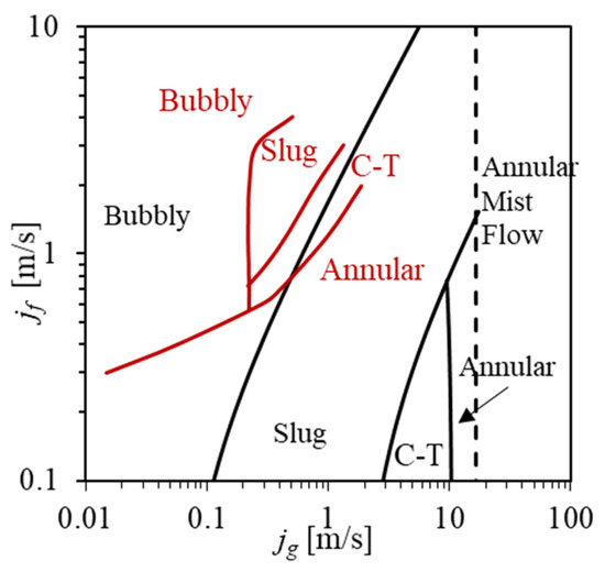
Figure 5.
Comparison of two-phase flow regimes of the VU flow by Mishima and Ishii [7] and VD flow by the authors [32].
Figure 6 and Figure 7 show the typical two-phase flow regimes observed in the VU direction [34] and in VD direction by the authors [31]. As can be seen, the shape and distribution of interfaces looks similar for all flow regimes for the VU and VD flows. Slight differences are observed for the bubbly flow and slug flow. The bubbles in the VU two-phase flow are in spherical or near spherical shapes and uniformly distributed across the pipe cross-section. Similar observation appears in Figure 7a in the VD two-phase flow. However, bubbly flow shows quiet different bubble distributions when increasing the liquid superficial velocity for a given gas superficial velocity, as shown in Figure 8. As can be observed, bubbles are uniformly distributed across the pipe cross-section for jf = 1.00 m/s. However, bubbles start to core at pipe center when the velocity jf is increased to 2.00 m/s. The so-called “coring phenomenon” still exists when increasing jf further. The core phenomenon has been observed and explained by Oshinowo and Charles [3] and Usui and Sato [4]. It is caused by the effect of buoyant force, which points towards the pipe center in VD flow. The lift force is propositional to the slip velocity between the gas phase and the liquid phase [35]. As jf increases, the slip velocity increases, resulting in a larger lift force. Consequently, more bubbles are pushed toward the pipe center and the coring phenomenon becomes more apparent.
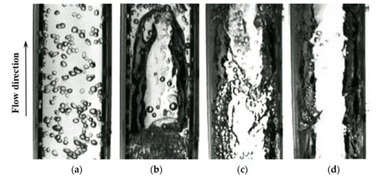
Figure 6.
Flow regimes observed in co-current VU two-phase flow in 50.8 mm round pipes. (a) Bubbly (b) Slug (c) Churn-turbulent (d) Annular.
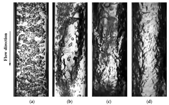
Figure 7.
Flow regimes observed in co-current VD two-phase flow in 50.8 mm round pipes. (a) Bubbly (b) Slug (c) Churn-turbulent (d) Annular.
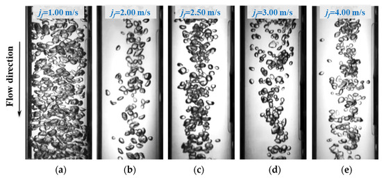
Figure 8.
Comparison of bubble distribution for and jg,loc = 0.08 m/s and increasing jf in VD bubbly flows. (a) Ref = 5 × 10⁴ (b) Ref = 105 (c) Ref = 1.25 × 10⁵ (d) Ref = 1.5 × 10⁵ (e) Ref = 2 × 10⁵.
For the slug flow shown by Figure 6b and Figure 7b both bullet-shaped slugs and liquid slugs occur alternately in the pipes, however, the slug bubbles is more distorted and has an off-centered nose in VD flow. This confirms the finding by Usui and Sato that the distortion of the bubble shape is more severe in the vertical downward flow as compared to the rising Taylor bubble in the steady liquid [4]. The difference in the slug shape can be explained by the phase interactions. The buoyance force accelerates the slug bubble in the VU flow but decelerates the slug bubble in the VD flow. Therefore, the interaction is more significant in VD flow than in VU flow, making a more distorted bubble. Interestingly, the nose of the slug in the VD flow is also pointing upward, same as the VU flow. The CT flow and annular flow look similar for VU and VD flows, but more droplets are observed in the pipe center, as shown by Figure 6c,d and Figure 7c,d.
3.2. Two-Phase Interfacial Structures
The characteristics of the interfacial structure can be represented by the void fraction, the interfacial area concentration, the bubble Sauter-mean diameter, the bubble velocity, and the bubble frequency. To reasonably compare the differences of the two-phase interfacial structures in different flow orientations, the experimental data for Run 2 in VU flow and Run 4 in VD flow are selected for comparison, since they have the same air and water superficial velocities at the fully developed axial locations of 61.5D and 55.5D, respectively.
Figure 9 compares the evaluation of local two-phase flow parameter distributions at different axial locations between the VU and VD flows. In the figure, lines with solid and empty dots represent the data measured in the VU and VD flows, respectively. It can be observed from Figure 9a that the α distributions in both the VU and VD flows are more or less symmetric in all measurement location. A center-peaked α distribution at 7.5D gradually develops into wall-peaked distribution as flowing upward in VU flow, which indicates that bubbles move toward the wall. For VD flow, however, the α distribution remains as center peaked at all three measurement locations. The difference is believed to be caused by the different direction of the lift force in VU and VD flows. According to the study by Saffman [36], the magnitude of the lift force is proportional to the product of the radial gradient of the axial continuous phase velocity and the relative velocity between the two phases. In VD flow, bubbles move slower than the liquid since the buoyant force is acting towards the opposite direction of the flow, while the opposite is observed in the VU flow. The direction of the lift force in VD flow points towards the pipe center, which is opposite to that in the VU flow. Therefore, bubbles migrate to the pipe wall in VU flow and to the pipe center in VD flow, with the help of the lift force.

Figure 9.
Comparison of interfacial structure parameters between VU (Run 2) and VD (Run 4) two-phase flows, (a) void fraction, (b) interfacial area concentration, (c) bubble Sauter-mean diameter, (d) bubble velocity, and (e) bubble frequency.
The ai distributions in Figure 9b show similar shapes as the α distributions in both the VU and VD flows. This is because the bubble are small in size and they remain spherical or near-spherical in bubbly flow, such that the ai value is proportional to α value. However, the evaluation of ai distributions is different from the evaluation of α distributions immediately downstream of 7.5D for both VU and VD flows. The α distributions remains similarly in all three locations in VD flow. However, ai decreases greatly from 7.5D to 31.5D, which is believed to be caused by the inlet effect. The bubble Sauter-mean diameter is about 1.5 mm at 7.5D, while it increases to around 2.5 mm at 31.5D, as shown in Figure 9c. Further, as can be seen from Figure 9e, the bubble frequency at 7.5D is significantly larger than the frequency at 31.5D. In other words, the bubble diameter is much smaller, and the bubble frequency is much larger at 7.5D than those at 31.5D, resulting in larger ai values at 7.5D. The small bubble diameter and large bubble frequency at 7.5D is believed to be caused by the sparger injector, which introduces many small bubbles. The ai values and its distribution after the second port remains almost unchanged, indicating that the flow is fully developed. Similar observations are found for the evaluation of ai in the VU flow.
The evolutions of vg distributions in VU and VD flows are shown in Figure 9d. In VU orientation, the flow is dominated by injection of the liquid phase at 7.5D, the vg profile is pretty flat at the pipe center, and it decreases near the wall. As the flow develops downstream, bubbles expand due to the pressure drop caused by the friction and acceleration. Meanwhile, bubbles are entrained by the continuous liquid phase and form a parabolic vg profile. In addition, the vg profile remains almost unchanged between 34.5D and 61.5D. The vg profile at 7.5D in the VD elbow, however, shows a double peaked distribution. This is speculated to be caused by combined effects of the local void fraction distribution and negative slip velocity between the gas and liquid phases. Since most of the bubbles are injected at the pipe center while the water is mainly injected near the wall, the water velocity is found to be smaller in the pipe center than that near the wall. Consequently, bubbles near the walls will move faster as entrained by the fast-moving water in the near wall region. Due to the entrainment by the liquid phase, the vg profile returns to parabolic shape downstream. Comparing the vg profiles of different flow orientation after 7.5D, it is found that the vg in VU flow is higher than that in VD flow, which demonstrates the effect of the buoyant force.
3.3. One-Dimensional Transport of Two-Phase Flow Parameters
The accuracy of the prediction by the one-dimensional system analysis code relies on precise modeling of the interfacial transfers. Therefore, evaluating the one-dimensional transport of the interfacial structure is necessary. Based on the detailed measured profiles, an area average is performed along the pipe diameter to get <α> and <ai>, and void-weighted area averages are performed to calculate <<Dsm>> and <<vg>>.
Figure 10 compares the evaluation of the one-dimensional two-phase flow parameters between VU and VD flows. The results of Run 2 and Run 3 in VU experiments and Run 4 and Run 5 in VD experiments are compared, since they belong to similar flow conditions. From Figure 10a, it can be observed that the evaluation of <α> in VU flow resembles VD flow, and <α> increase along the flow direction. This is counterintuitive as the net pressure decreases in VU flow but increases in VD flow; a decrease in <α> is expected in VD flow since increasing pressure will compress bubbles. However, the variation of <α> is actually determined by the combined effects of pressure change and advection of the gas phase considering the one-dimensional gas phase continuity equation. Bubble deceleration can cause the accumulation of bubbles and increase the void fraction. The decrease in <<vg>> for Run 4 and Run 5 in VD flows as shown in Figure 10d, will cause a net increase in <α>. From Figure 10b, the evaluation of <ai> is similar for VU and VD flows. The flows investigated remain in bubbly flow regime and bubbles are near-spherical, therefore, the evaluation of <ai> is linearly proportional to the evaluation of <α>. The initial decrease in <ai> for both orientations is caused by the coalescence of the small size bubbles generated by the injector, as reflected by the increase in <<Dsm>> in Figure 10c. The latter increase downstream is the consequence of the <α> increase and bubble interactions.
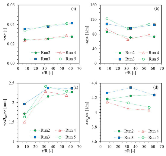
Figure 10.
Comparison of area-averaged interfacial parameters between VU and VD two-phase flows, (a) void fraction, (b) interfacial area concentration, (c) bubble Sauter-mean diameter, and (d) bubble velocity.
Figure 10c,d plot the evaluation of <<Dsm>> and <<vg>> in VU and VD flows. <<Dsm>> increases initially but varies differently in the downstream for VU and VD flows. As mentioned earlier, the initial increase in <<Dsm>> is caused by the inlet effect. In the downstream, <<Dsm>> does not change too much beyond 34.5D in VU flow but decreases beyond 31.5D in VD flow. This indicate a higher turbulent coalescence effect in VD flow than in VU flow, which is understandable as the buoyant force is opposite to the flow direction and turbulent induced interaction is promoted in VD flow. <<vg>> almost linearly increases with the development length for Run 2 in VU flow but shows an unexpected decrease between 34.5D and 61.5D for Run 3. The difference may be caused by the measurement uncertainty. <<vg>> for Run 4 and Run 5 decrease consistently with the flow development, since buoyant force impedes the downward flowing bubbles and promotes phase interactions. This highlights the different effect of buoyant force on VU and VD two-phase flows.
3.4. Frictional Pressure Drop
Due to the differences in interfacial structures of two-phase VU and VD flows, the variation of frictional pressure drop shows different characteristics, such that different models or model coefficients are required for predicting the two-phase flow frictional pressure drop in different flow orientation. The Lockhart–Martinelli correlation is based on the assumption that the two-phase frictional pressure drop is the sum of the pressure drops caused by each individual phase, i.e., the total frictional pressure drops equals the liquid-phase pressure drop plus the gas-phase pressure drop and a term accounting for the interactions between the two phases, which is evaluated by Equation (3) [37]. The coefficient C in Equation (3) is an adjustable parameter which quantifies the coupling effects between the two phases [37]. The C value of 20 has demonstrated capability in predicting the two-phase pressure drop in horizontal flows [38]. However, no consensus C value is reached for the other flow orientations.
In Equation (3), is the two-phase multiplier, X2 is the Lockhart–Martinelli parameter, and (dp/dz) terms are the pressure drop by each individual phase or the two-phase mixture.
The Lockhart–Martinelli correlation is used to predict the two-phase flow frictional pressure drop in VU and VD flows. As shown in Figure 11, it is interesting to see that the value is larger in VU flow than in VD flow, indicating that the pressure drop is larger in VU flow than in VD flow. The recommended C value of 20 can predict the frictional pressure drop in VD flow with a relative error of 1%. In VU flow, however, an increased C value of 50 is needed to predict the pressure drop with a relative error of approximately 1%. Though the determined C values are based on the limited data and may be limited to the current test configurations, it demonstrates the differences in frictional pressure drop in VU and VD two-phase flows. This suggests different models or model coefficients are needed when predicting two-phase frictional pressure drops in different flow orientations.
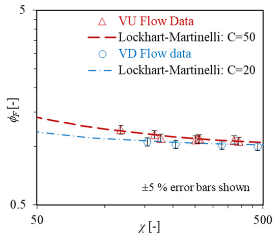
Figure 11.
Frictional pressure loss analysis for VU and VD flows using the Lockhart–Martinelli correlation.
4. Summary and Conclusions
In the present study, the effects of flow orientation on the global and local two-phase flow parameters are studied experimentally. Characteristics of flow regimes and interfacial structures, and frictional pressure loss in the vertical upward and vertical downward two-phase flows are compared and analyzed. Following conclusions are reached.
- (1)
- The general characteristics of the flow regimes for the vertical upward and vertical downward flows are similar. In the vertical downward flow, bubbles tend to core in the pipe center under high liquid superficial velocity conditions due to the lift force effect, and slugs have an off-centered nose.
- (2)
- All flow regime transition boundaries in the vertical downward flow are shifted to the lower gas superficial velocities compared to that in the vertical upward flow, because of the significant bubble interaction and coalescence promoted by the buoyant force, lift force, and the coring phenomenon in vertical downward flows.
- (3)
- The profiles of the void fraction and interfacial area concentration show wall-peaked distribution in the vertical upward bubbly flow but center-peaked distribution in the vertical downward bubbly flow, which is caused by the opposite direction of the lift force.
- (4)
- The area-averaged void fraction increase is due to the pressure decrease in the vertical upward flow but caused by the deceleration of bubbles in the vertical downward flow. The void-weighted area-averaged bubble velocity decreases in the vertical downward flow due to the buoyancy effect.
- (5)
- The pressure drop is larger in the vertical upward flow than that in the vertical downward flow. The recommended C value of 20 for the Lockhart–Martinelli correlation can predict the frictional pressure drop in the vertical downward flow with a relative error of 1%, while an increased C value of 50 is required to predict the pressure drop in the vertical upward flow with similar accuracy.
Author Contributions
Writing—original draft, S.Q., data curation, S.Q.; editing, J.L. and J.R.; supervision, S.K., methodology, S.K. All authors have read and agreed to the published version of the manuscript.
Funding
This work is financially supported by National Natural Science Foundation of China (11905039), and the China Postdoctoral Science Foundation (2021T140148, 2019M651267).
Institutional Review Board Statement
Not applicable.
Informed Consent Statement
Not applicable.
Data Availability Statement
Not applicable.
Conflicts of Interest
The authors declare no conflict of interest.
References
- Mandhane, J.M.; Gregory, G.A.; Aziz, K. A flow pattern map for gas—Liquid flow in horizontal pipes. Int. J. Multiph. Flow 1974, 1, 537–553. [Google Scholar] [CrossRef]
- Qiao, S.; Kim, S. Air-water two-phase bubbly flow across 90° vertical elbows. Part I: Experiment. Int. J. Heat Mass Transf. 2018, 123, 1221–1237. [Google Scholar] [CrossRef]
- Oshinowo, T.; Charles, M.E. Vertical two-phase flow part I. Flow pattern correlations. Can. J. Chem. Eng. 1974, 52, 25–35. [Google Scholar] [CrossRef]
- Usui, K.; Sato, K. Vertically downward two-phase flow, (I). J. Nucl. Sci. Technol. 1989, 26, 670–680. [Google Scholar] [CrossRef]
- Goda, H.; Kim, S.; Mi, Y.; Finch, J.P.; Ishii, M.; Uhle, J. Flow Regime Identification of Co-Current Downward Two-Phase Flow with Neural Network Approach. In Proceedings of the 10th International Conference on Nuclear Engineering, Arlington, VA, USA, 14–18 April 2002; Volume 3, pp. 71–78. [Google Scholar] [CrossRef]
- Taitel, Y.; Bornea, D.; Dukler, A.E. Modelling flow pattern transitions for steady upward gas-liquid flow in vertical tubes. AIChE J. 1980, 26, 345–354. [Google Scholar] [CrossRef]
- Kaichiro, M.; Ishii, M. Flow regime transition criteria for upward two-phase flow in vertical tubes. Int. J. Heat Mass Transf. 1984, 27, 723–737. [Google Scholar] [CrossRef]
- Barnea, D.; Shoham, O.; Taitel, Y. Flow pattern transition for vertical downward two phase flow. Chem. Eng. Sci. 1982, 37, 741–744. [Google Scholar] [CrossRef]
- Jiang, Y.; Rezkallah, K.S. A Study on void fraction in vertical co-current upward and downward two-phase gas-liquid flow—I: Experimental results. Chem. Eng. Commun. 1993, 126, 221–243. [Google Scholar] [CrossRef]
- Milan, M.; Borhani, N.; Thome, J.R. Adiabatic vertical downward air-water flow pattern map: Influence of inlet device, flow development length and hysteresis effects. Int. J. Multiph. Flow 2013, 56, 126–137. [Google Scholar] [CrossRef]
- Kazi, J.; Fukuma, J.; Kurimoto, R.; Hayashi, K.; Tomiyama, A. Void fractions in U-bends of a serpentine tube. Multiph. Sci. Technol. 2022, 34, 41–55. [Google Scholar] [CrossRef]
- Serizawa, A.; Kataoka, I.; Michiyoshi, I. Turbulence structure of air-water bubbly flow—II. Local properties. Int. J. Multiph. Flow 1975, 2, 235–246. [Google Scholar] [CrossRef]
- Liu, T.; Bankoff, S. Structure of air-water bubbly flow in a vertical pipe—II. Void fraction, bubble velocity and bubble size distribution. Int. J. Heat Mass Transf. 1993, 36, 1061–1072. [Google Scholar] [CrossRef]
- Wang, S.; Lee, S.; Jones, O.; Lahey, R. 3-D turbulence structure and phase distribution measurements in bubbly two-phase flows. Int. J. Multiph. Flow 1987, 13, 327–343. [Google Scholar] [CrossRef]
- Ishii, M.; Paranjape, S.; Kim, S.; Sun, X. Interfacial structures and interfacial area transport in downward two-phase bubbly flow. Int. J. Multiph. Flow 2004, 30, 779–801. [Google Scholar] [CrossRef]
- Hibiki, T.; Goda, H.; Kim, S.; Ishii, M.; Uhle, J. Experimental study on interfacial area transport of a vertical downward bubbly flow. Exp. Fluids 2003, 35, 100–111. [Google Scholar] [CrossRef]
- Hibiki, T.; Goda, H.; Kim, S.; Ishii, M.; Uhle, J. Structure of vertical downward bubbly flow. Int. J. Heat Mass Transf. 2004, 47, 1847–1862. [Google Scholar] [CrossRef]
- Kim, S.; Paranjape, S.S.; Ishii, M.; Kelly, J. Interfacial Structures and Regime Transition in Co-Current Downward Bubbly Flow. J. Fluids Eng. 2004, 126, 528–538. [Google Scholar] [CrossRef]
- Kim, S. Interfacial Area Transport Equation and Measurement of Local Interfacial Characteristics; Purdue University: West Lafayette, IN, USA, 1999. [Google Scholar]
- Sun, X.; Smith, T.R.; Kim, S.; Ishii, M.; Uhle, J. Interfacial structure of air-water two-phase flow in a relatively large pipe. Exp. Fluids 2003, 34, 206–219. [Google Scholar] [CrossRef]
- Goda, H.; Kim, S.; Paranjape, S.S.; Finch, J.P.; Ishii, M.; Uhle, J. Local Interfacial Structure in Downward Two-Phase Bubbly Flow. In Proceedings of the 10th International Conference on Nuclear Engineering, Arlington, VA, USA, 14–18 April 2002; Volume 3, pp. 115–121. [Google Scholar]
- Hibiki, T.; Goda, H.; Kim, S.; Ishii, M.; Uhle, J. Axial development of interfacial structure of vertical downward bubbly flow. Int. J. Heat Mass Transf. 2005, 48, 749–764. [Google Scholar] [CrossRef]
- Todreas, N.E.; Kazimi, M.S. Nuclear Systems; Taylor & Francis: London, UK, 2012; Volume 2, ISBN 9781439808887. [Google Scholar]
- Lockhart, R.W.; Martinelli, R.C. Proposed correlation of data for isothermal two-phase, two-component flow in pipes. Chem. Eng. Prog. 1949, 45, 39–48. [Google Scholar]
- Bhagwat, S.M.; Ghajar, A.J. Similarities and differences in the flow patterns and void fraction in vertical upward and downward two phase flow. Exp. Therm. Fluid Sci. 2012, 39, 213–227. [Google Scholar] [CrossRef]
- Jiang, Y.; Rezkallah, K.S. A Study on void fraction in vertical co-current upward and downward two-phase gas-liquid flow—II: Correlations. Chem. Eng. Commun. 1993, 126, 245–259. [Google Scholar] [CrossRef]
- Tian, D.; Yan, C.; Sun, L.; Tong, P.; Liu, G. Comparison of local interfacial characteristics between vertical upward and downward two-phase flows using a four-sensor optical probe. Int. J. Heat Mass Transf. 2014, 77, 1183–1196. [Google Scholar] [CrossRef]
- Zeguai, S.; Chikh, S.; Tadrist, L. Experimental study of air-water two-phase flow pattern evolution in a mini tube: Influence of tube orientation with respect to gravity. Int. J. Multiph. Flow 2020, 132, 103413. [Google Scholar] [CrossRef]
- Abdulkadir, M.; Kajero, O.T.; Olarinoye, F.O.; Udebhulu, D.O.; Zhao, D.; Aliyu, A.M.; Al-Sarkhi, A. Investigating the Behaviour of Air–Water Upward and Downward Flows: Are You Seeing What I Am Seeing? Energies 2021, 14, 7071. [Google Scholar] [CrossRef]
- Chalgeri, V.S.; Jeong, J.H. Flow patterns of vertically upward and downward air-water two-phase flow in a narrow rectangular channel. Int. J. Heat Mass Transf. 2018, 128, 934–953. [Google Scholar] [CrossRef]
- Qiao, S.; Mena, D.; Kim, S. Inlet effects on vertical-downward air–water two-phase flow. Nucl. Eng. Des. 2017, 312, 375–388. [Google Scholar] [CrossRef]
- Kim, S.; Fu, X.; Wang, X.; Ishii, M. Development of the miniaturized four-sensor conductivity probe and the signal processing scheme. Int. J. Heat Mass Transf. 2000, 43, 4101–4118. [Google Scholar] [CrossRef]
- Wu, Q.; Ishii, M. Sensitivity study on double-sensor conductivity probe for the measurement of interfacial area concentration in bubbly flow. Int. J. Multiph. Flow 1999, 25, 155–173. [Google Scholar] [CrossRef]
- Yadav, M.S. Interfacial Area Transport Across Vertical Elbows in Air-Water Two-Phase Flow; The Pennsylvania State University: State College, PA, USA, 2013. [Google Scholar]
- Ishii, M. Thermo-Fluid Dynamic Theory of Two-Phase Flow; Collection de la Direction des Etudes et Recherches d’Electricite de France; Eyrolles: Paris, France, 1975; ISBN 978-1-4419-7984-1. [Google Scholar]
- Saffman, P.G. The Lift on a Small Sphere in a Slow Shear Flow. J. Fluid Mech. 1965, 22, 385–400. [Google Scholar] [CrossRef]
- Kim, S.; Kojasoy, G.; Guo, T. Two-phase minor loss in horizontal bubbly flow with elbows: 45° and 90° elbows. Nucl. Eng. Des. 2010, 240, 284–289. [Google Scholar] [CrossRef]
- Chisholm, D. A theoretical basis for the Lockhart-Martinelli correlation for two-phase flow. Int. J. Heat Mass Transf. 1967, 10, 1767–1778. [Google Scholar] [CrossRef]


Disclaimer/Publisher’s Note: The statements, opinions and data contained in all publications are solely those of the individual author(s) and contributor(s) and not of MDPI and/or the editor(s). MDPI and/or the editor(s) disclaim responsibility for any injury to people or property resulting from any ideas, methods, instructions or products referred to in the content. |
© 2022 by the authors. Licensee MDPI, Basel, Switzerland. This article is an open access article distributed under the terms and conditions of the Creative Commons Attribution (CC BY) license (https://creativecommons.org/licenses/by/4.0/).