Article

A Novel Anomaly Detection Method for Strip Steel Based on Multi-Scale Knowledge Distillation and Feature Information Banks Network

1
School of Software, Shenyang University of Technology, Shenyang 110870, China
2
School of Mechanical Engineering & Automation, Northeastern University, Shenyang 110819, China
*
Author to whom correspondence should be addressed.
Coatings 2023, 13(7), 1171; https://doi.org/10.3390/coatings13071171
Submission received: 25 May 2023 / Revised: 25 June 2023 / Accepted: 26 June 2023 / Published: 28 June 2023
(This article belongs to the Section Laser Coatings)

Abstract

:
To address the problem of image imbalance in the surface inspection of strip steel, this study proposes a novel anomaly detection method based on multi-scale knowledge distillation (Ms-KD) and a block domain core information module (BDCI) to quickly screen abnormal images. This method utilizes the multi-scale knowledge distillation technique to enable the student network to learn the ability to extract normal image information under the source network pre-trained on ImageNet. At the same time, the optimal storage of block-level features is used to extract low-level and high-level information from intermediate layers and establish a feature bank, which is searched for core subset libraries using a greedy nearest neighbor selection mechanism. By using the Ms-KD module, the student model can understand the abnormal data more comprehensively so as to better capture the information in the data to solve the imbalance of abnormal data. To verify the validity of the proposed method, a completely new dataset called strip steel anomaly detection for few-shot learning (SSAD-FSL) was constructed, which involved image-level and pixel-level annotations of surface defects on cold-rolled and hot-rolled strip steel. By comparing with other state-of-the-art methods, the proposed method performs well on image-level area under the receiver operating characteristic curve (AUROC), reaching a high level of 0.9868, and for pixel-level per region overlap (PRO) indicators, the method also achieves the best score of 0.9896. Through a large number of experiments, the effectiveness of our proposed method in strip steel defect anomaly detection is fully proven.

1. Introduction

The detection of strip steel surface defects is a crucial step in the production process because of defects on the surface of strip steel, such as cracks, skin oxidation, punch holes and more. These defects will directly affect the quality and performance of the product and even cause adverse production accidents. The traditional defect detection method has a slow detection speed and cannot meet the requirements of efficient detection. In particular, some complex defects rely on professional detection, which has certain subjectivity, low missed detection and a false detection rate. Machine vision inspection technology based on deep learning has been widely used in the detection of defects on metal surfaces [1,2,3], pavement surfaces [4,5,6] and other materials [7,8,9]. The detection method based on deep learning has a strong representation ability by learning features from a large number of training samples. Deep learning theory includes a variety of network models, such as multilayer perceptrons (MLPs) [10], convolutional neural networks (CNNs) [11], recurrent neural networks (RNNs) and generative adversarial networks (GANs) [12]. These different network models are suitable for different scenarios. Deep learning models based on convolutional neural networks have achieved great success in various computer vision fields, such as face recognition, pedestrian recognition and text detection in images. Furthermore, these models are used in a wide range of industrial settings for defect detection [13,14].
Although anomaly detection has gradually become more perfect and mature in many fields, there are still some challenges in the application of complex industrial scenarios. With the increasing demand for intelligent manufacturing, the inconsistency between the incompleteness of industrial big data anomaly detection research and the increasing demand has become a serious bottleneck restricting the intelligent process of industrial production and manufacturing. The following challenges are included in the constructed defect detection dataset, as shown in Figure 1.
  • Rareness of abnormal data: This refers to the scarcity of accurately labeled abnormal data in industrial data. Obtaining accurate pixel-level annotations requires professional skilled workers to sketch, which is costly. In contrast, the labeling cost of natural images is low.
  • The imbalance of abnormal data: a. At the image level, the number of normal industrial images is far more than that of abnormal ones, which is caused by different production and processing conditions. b. At the pixel level, the collected abnormal area occupies a small pixel area on the entire surface image, which leads to very high similarity between normal and abnormal samples.
  • The diversity of anomaly characterization: Industrial image anomalies often have a variety of different sizes, shapes, locations and texture features. From a statistical point of view, the data distribution of these anomalies is inconsistent. Therefore, there are still some challenges in the application of quality control and surface defect localization.
In order to solve the above problems, this paper proposes an anomaly detection method based on multi-scale knowledge distillation and feature information banks.
The main contributions of this article are summarized as follows.
(1)
This paper proposes a novel unsupervised anomaly detection method based on distillation learning. This method uses a better pre-training network to learn the distribution pattern of normal images and analyzes the difference in image processing through the teacher–student model. It can accurately identify unknown abnormal data and effectively solve the problem of unknown anomaly detection.
(2)
In this paper, a new dataset SSAD-FSL (strip steel anomaly detection for few-shot learning) is established, including 3000 grayscale images with a resolution of 224 × 224. The construction of the dataset includes image-level and pixel-level labeling of surface defects of cold-rolled strip steel and hot-rolled strip steel.
(3)
In the test process, the abnormal score is calculated by calculating the distance between the test sample and the nearest neighbor sample in the feature banks so as to realize the task of distinguishing and locating the defects. The experimental results show that the proposed anomaly detection algorithm can effectively screen out the defect samples and perform better than other similar models.

2. Related Works

In the task of image anomaly detection, it can be divided into two categories according to the feature of anomaly morphology: qualitative anomaly classification and quantitative anomaly location. It was first implemented by a series of traditional methods [15,16]. Later, unsupervised or semi-supervised learning methods were used to detect abnormal images or local abnormal regions different from normal images through deep learning methods. Deep learning technology is widely used in image anomaly detection tasks, including methods based on distance measurement, classification surface construction and image reconstruction.

2.1. Anomaly Detection Method Based on Distance Measure

The core idea of distance-based methods, such as deep support vector data description (SVDD) [17] and k-nearest neighbor algorithms (AMSD-kNNs [18]), is to train deep neural networks to make the feature vectors extracted from normal images more compact and to calculate the distance between the sample to be tested and the normal features to measure the degree of abnormality. In [19,20], a support vector machine is applied to surface defect detection tasks. However, such methods are not effective for complex datasets and are prone to model degradation.

2.2. Anomaly Detection Method Based on Constructing Classification Surface

The key concept behind the anomaly detection approach that is based on constructing classification boundaries is to transform a singular normal sample into multiple class samples and to construct the classification surface in the image space by training the classifier so as to realize the classification of normal samples and potential abnormal samples. Deep robust one-class classification (DROCC) proposed by Goyal [21] and Golan [22] used flip, translation and rotation to construct a classification dataset containing 72 categories to train the classification network. The advantage of these methods is that they can flexibly handle complex data distribution and can detect different types of abnormal samples. The anomaly detection method based on constructing a classification surface has the disadvantage of dependence on the distribution of abnormal samples. The anomaly detection method based on constructing a classification surface usually classifies normal and abnormal samples by learning a classifier or classification boundary based on the distribution difference between normal samples and abnormal samples. This means that these methods have limited assumptions about the distribution and number of abnormal samples. If the distribution of abnormal samples is similar to normal samples or the number of abnormal samples is very limited, the classification surface may not be able to accurately distinguish abnormal samples.

2.3. Anomaly Detection Method Based on Image Reconstruction

An anomaly detection method based on image reconstruction aims to learn the distribution pattern of normal images by encoding and decoding normal images. When detecting, anomaly detection is performed by analyzing the difference between the images before and after reconstruction. Methods based on image reconstruction usually include two types based on autoencoder and generative adversarial networks (GANs).
An autoencoder is an unsupervised learning neural network composed of an encoder and decoder. The encoder compresses the input data into a low-dimensional code, and the decoder restores the encoding and decoding to the original form. It learns data representations by minimizing reconstruction errors and can be based on different types of neural networks. The backpropagation algorithm is used to train the model and restore the original data. The difference between the input data and the reconstructed data is considered to be an outlier. Gong et al. [23] proposed the MemAE method, which learns the potential features of data in feature extraction, thereby improving the performance of classification and clustering.
A GAN is a deep learning model proposed by Goodfellow in 2014 which consists of two neural networks: a generator and discriminator. The generator generates new data similar to real data through random noise, and the discriminator tries to distinguish the newly generated data from the real data. The training process has multiple confrontations, helping the generator learn the distribution of real data, and the resulting data is becoming more and more realistic. Samet and Amir et al. [24] relied on the GAN to let the model learn to characterize high-dimensional images and their data distribution in latent space. Various network models of GANs are used for anomaly detection, such as the AnoGAN [25] and OCGAN [26].
Anomaly detection methods based on image reconstruction rely too much on normal data training. Anomaly detection methods for image reconstruction usually need to be trained with normal data to learn the features and patterns of normal images. This means that the performance of the method may be limited if the training data is insufficient or there are abnormal samples in the training data. In addition, the performance of the model may also degrade if the distribution of normal data changes in the test data.
In unsupervised anomaly detection where only normal samples can be used as training data, most solutions are to employ one-class classification, such as deep one-class networks [27], which are able to learn a discriminative hyperplane around normal samples. In addition, in the unsupervised clustering method, the Gaussian mixture model (GMM) [28] is used to build a detailed profile of normal data to identify anomalies. These methods perform poorly when dealing with high-dimensional data.
Although there is a lot of research on image anomaly detection tasks, there are still many problems that have not been fully explored. Most anomaly detection methods use image reconstruction or classification surface construction to detect abnormal images, but these detection methods do not consider the problem of image sample imbalance and the limited representation ability of abnormal samples, resulting in the decline of anomaly detection performance. In order to solve these problems, we propose an unsupervised anomaly detection method based on multi-scale knowledge distillation (MKD-IR). This method adopts a multi-scale knowledge distillation model, which can reduce the amount of data computation and make full use of the low-level and high-level information of normal data. In addition, the block domain feature information database module is used to effectively suppress the tendency of the model to extract the features of natural image data and improve the sensitivity of the model to abnormal data.
The comparison of anomaly detection techniques under different methods is shown in Table 1.

3. Methodology

3.1. Methodology Overview

This paper proposes an unsupervised anomaly detection method for anomaly detection and location of strip steel surfaces. The method consists of two main components: the multi-scale knowledge distillation module (Ms-KD) and block domain core information banks module (BDCI). The overall framework of the method is shown in Figure 2.
First, the normal strip steel surface images are input into the two main branches of the Ms-KD module. The knowledge of the source network pre-trained on ImageNet is distilled into a simpler student network. By combining low-level features and high-level features obtained under different convolutional layers, the student network can deeply learn the information of normal images. The simple and compact student model can avoid distraction due to non-distinguishing features and enhance the ability to distinguish normal and abnormal features. When the student network completely transfers the knowledge of the source program, some intermediate-level features are stored in a specific memory bank in a block domain, which stores the core information of normal data. We use a greedy neighbor selection mechanism to find the core subset, reduce the amount of data and minimize the impact of detection results. The memory bank is core sampled, ensuring low inference cost but higher performance. When a test set containing a mixture of normal and abnormal data is input into the network, the network will access all stored normal data information and evaluate the abnormal score by measuring the distance of the corresponding features. This method uses block domain feature scores to explain spatial differences and reduces network bias against natural image classes.

3.2. Ms-KD Module

One of the core components of this method is the Ms-KD module, which is based on the idea of distillation learning. Multi-scale knowledge distillation is a deep learning technique that trains multiple models at different scales by combining them together. It aims to transfer the knowledge of a complex teacher model to a simpler student model. This approach can improve the performance of the student model and enable it to generalize better.
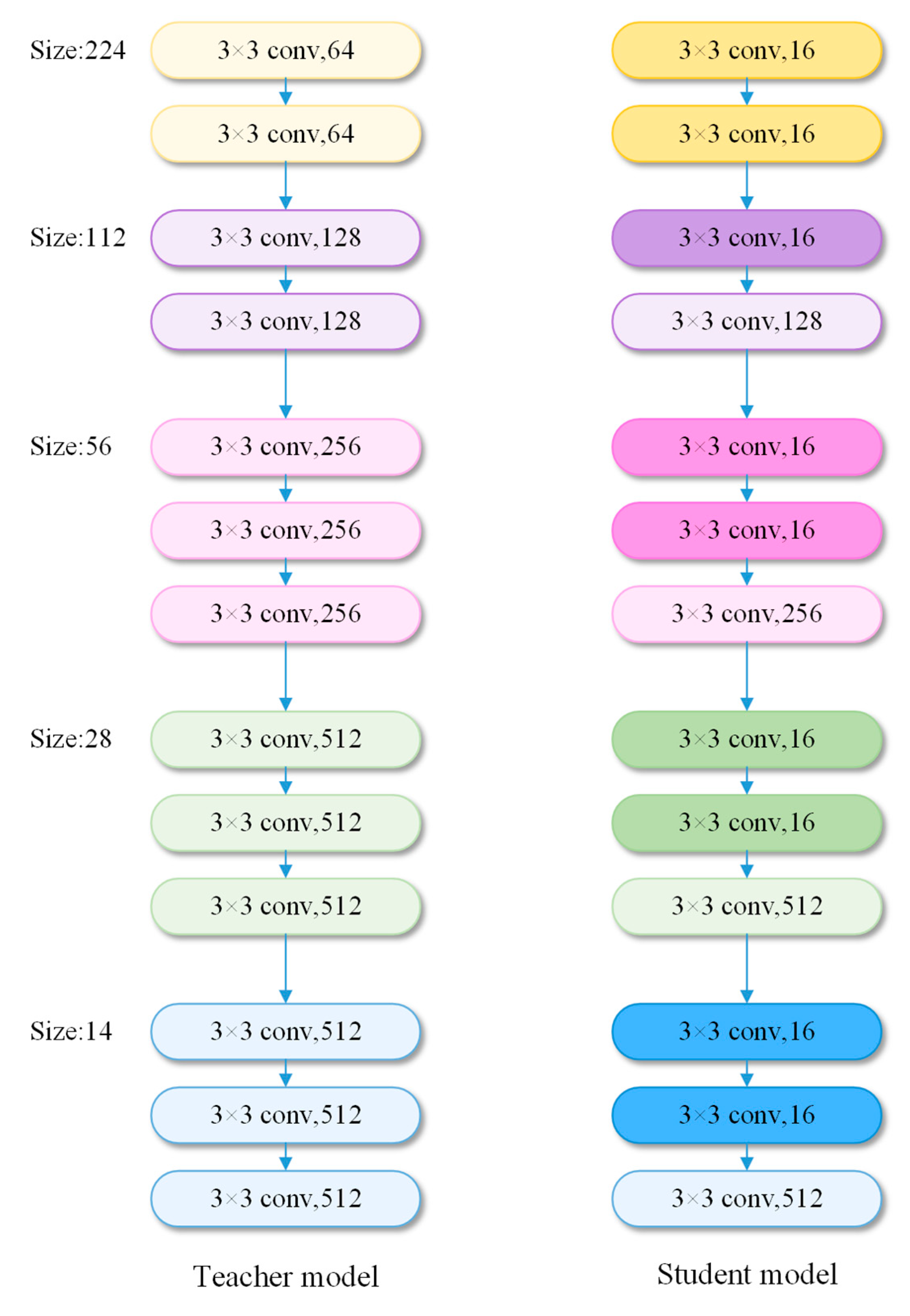
The method uses a large teacher model pre-trained on the ImageNet dataset to provide knowledge and uses a simplified, small student model to learn the knowledge of the teacher model and continuously optimize itself. The parameters of the teacher model are frozen, and the strip steel surface image with a size of H × W × C is input into the backbone network for feature extraction, and the final output feature map size is H 32 × W / 32 × C 5 ; at the same time, the student model also performs feature extraction in the same way, as shown in Figure 3.
The purpose of this method is to train a student model that can detect abnormal images in the test data. The teacher model uses the VGG-16 network, while the student model uses a simplified VGG network with fewer parameters. Since the training set only includes normal images without abnormal images, it is necessary to use the intermediate knowledge of teacher model on normal data to guide the training of student model.
In order to achieve this goal, this method not only uses the output features of the last layer but also transmits the edge features of the basic layer and the semantic features of different abstract levels of the middle layer to the student model. In this way, the student model can understand the normal data more comprehensively, thereby improving the accuracy of detecting abnormal images. In order to save computing costs and memory usage, this paper still uses feature distillation for training. By using this technique, the student model can focus more on learning the main features and output distribution of normal images so as to better capture the information in the data. By compressing the source code, this technique can prevent features that cannot be distinguished between normal and abnormal data from interfering with the learning process.

3.3. BDCI Module

Another core component of the method is the BDCI module; its main idea is to divide the feature map information of the training normal data into several regions and store them in blocks. Then, the greedy approximation algorithm is used to find the optimal sub-library. In the test phase, anomalies can be detected by comparing the differences between test data and information bank features.

3.3.1. Block Domain Feature Selection

Distillation learning is a pre-trained network on the ImageNet dataset. Therefore, the network focuses more on learning the features of abstract natural image datasets in the training process, and the correlation with strip steel industrial anomaly detection tasks and evaluation data is very limited. Therefore, the model is very unfavorable for the downstream strip steel surface defect classification task. In addition, unknown and variable exception types are often encountered during testing, which further increases the difficulty of model detection accuracy. In order to improve the detection accuracy of the model, this paper adopts another method.
The method in this paper chooses a strategy to process the features whose accuracy is close to the teacher model in the student model, extracts the core by block domain and stores it in the specified feature bank. In order to avoid feature knowledge that is too general or biased towards natural image classification, the intermediate or intermediate feature representation is selected. This feature representation is more general, suitable for a wider range of tasks and reduces the dependence on the feature knowledge of natural image classification. This strategy helps to improve the generalization performance of the model and can effectively reduce the use of storage space.
Specifically, the selection of block domain features is based on the student model S ψ that completes knowledge distillation. The features on the specific network layer play an important role, and the intermediate features are expressed as S ψ i , j = S ψ j x i , x i D (Dataset D). In this method, j 1 , 2 , 3 , 4 , 5 are the number of levels in the S ψ network where the feature is located. S ψ i , j R h * × w * × c * is a three-dimensional tensor. Its depth is c * , height is h * and width is w * .
The c * -dimensional block domain feature at position h 1 , , h * , w 1 , , w *   is denoted by S ψ i , j h , w = S ψ j x i , h , w R c * . In the case of setting, the extraction of block domain features is completed under a large enough receptive field. In order to capture the complex structure and pattern involving local so as to improve the understanding and perception of local visual information.
Block domain features are crucial to stimulate local neighborhood aggregation. They can increase the size of the receptive field and improve the robustness to small spatial deviations without losing the spatial resolution or availability of the feature map. In order to better explain this phenomenon, the previously mentioned symbol S ψ i , j h , w is extended to explain the uneven block domain size.
N m h , w = a , b a h m / 2 , , h + m / 2 , b w m / 2 , , w + m / 2
Local features in h , w can be expressed as:
S ψ i , j N m h , w = f a g g ψ i , j a , b a , b N m h , w
f a g g is an aggregation function, and the obtained feature vectors are clustered near N m h , w . The method in this paper uses an adaptive average pooling operation. A representation of h 1 , , h * , w 1 , , w * with dimension d is generated at h , w , which preserves the resolution of the feature map. In summary, for a feature map tensor S ψ i , j , the block domain feature set B n , m S ψ i , j is:
B n , m S ψ i , j = S ψ i , j N m h , w h , w mod n = 0 , h < h , w < w , h , w N
In order to retain the feature information used, this method uses two intermediate feature layers j and j + 1 in the student model. For all training samples x i D t r a i n , each element is aggregated with its corresponding block domain features, and the corresponding feature repository B A N K is defined as:
B A N K = x i D t r a i n B n , m S ψ j x i

3.3.2. Core Repository

B A N K is proportional to the size of D t r a i n . The increasing training data will lead to an increasing amount of data to be stored, and the time of testing and reasoning will become longer. Therefore, this method uses a core set sampling mechanism to reduce the amount of B A N K data.
The purpose of core set selection is to find a subset S A so that the solution to the problem on this subset can be the nearest solution on the complete dataset A , especially the solution on the complete dataset that can be approximated more quickly. Since different problems may have different requirements for core values, the core values of interest will also vary from problem to problem. In order to ensure that the coverage of the selected core set B A N K C * is roughly similar to that of the original complete dataset B A N K in the block domain level feature space, this paper uses the minimax method to select it.
B A N K C = arg min B A N K C B A N K max p B A N K min q B A N K p q 2
The exact calculation of B A N K C * comes from the iterative greedy approximation in NP-Hard [29]. In order to further reduce the selection time of the core set, the Johnson–Lindenstrauss theorem [30] is used to reduce the number of dimensions d * < d by making R d R d * by random linear projection. This method has been used for a long time in basic KNN and Kmeans methods or hybrid models by finding the subset closest to some available sets and allowing for finding approximate solutions at a significantly reduced cost. The process is shown in Algorithm 1.
Algorithm 1: The flow of building a block domain core information bank.
Coatings 13 01171 i001

3.4. Loss Design

In this paper, the i intermediate layer of the distillation learning network is defined as f T i and f S i ( f T 0   and f S 0 represent the original input), the source activation value of the intermediate layer of the teacher model is a T f T i and the layer activation function value learned by the student model is a S f S i . As the meaning of knowledge distillation, feature knowledge refers to the output value of the activation layer. In this method, two loss functions are defined to constrain the knowledge transfer of the teacher model to the student model. One is L M I D between different intermediate layers, which aims to minimize the Euclidean distance between the activated output values of each layer. The second L A L L is the integration of losses from different intermediate layers at the end of the output layer of the network. The specific calculation process is shown in Formulas (6) and (7).
L M I D = a T f T i ( j ) a S f S i ( j ) 2
j is the j t h activation value of f T i or f S i .
At the end of the input layer, the loss functions of the above different intermediate layers are integrated. Using this loss function makes L A L L training continue to converge, which is an available criterion for measuring when to stop training.
L A L L = i = 1 N f 1 N i a T f T i ( j ) a S f S i ( j ) 2 = i = 1 N f 1 N i j = 1 N l L M I D
where N f is the number of neurons in the a S f S i a layer, and N l is the total number of key layers.

3.5. Training Configurations

Visual geometry group 16 (VGG16) is a deep convolutional neural network that is commonly used with its pre-trained model as a feature extractor for image classification and object recognition tasks. In this paper, VGG16 is used as the backbone of the teacher network, its final fully connected layer is removed and the features of different levels are extracted so that the student network can learn more accurate target features. During training, the pre-training weights obtained on the ImageNet dataset are first loaded into VGG16, and then the training images (normal images) are input into the two networks. Given a training dataset D t r a i n = x 1 , , x n | y x i = 0 composed of normal images (i.e., there is no anomaly), a clone network student model is finally trained, which detects abnormal images in the test set D t e s t and locates anomalies in these images. Specifically, the output of 3, 6, 9, and 12 layers of the teacher model and student model is used as the real label and the prediction label, respectively, and the loss value is calculated. Finally, the backpropagation and iterative operation are carried out. In the final epoch stage of training, the patch features of normal images carry embedding vectors of information from different semantic levels and resolutions, which will be stored in the repository.
The VGG network shows good performance in classification and transfer learning, showing its practicability in different image processing fields. The method in this paper uses the difference in extracted image features between the teacher model and student model to find anomalies. In the teacher model, in the output of the last four layers of each convolution block, the maximum pooling layer is selected as the critical point ( L Q i t ).
In order to avoid the use of bias terms in the student model network, for some layers between any L Q , such as i t h and i 1 t h , the student model can generate a specific constant activation vector a T L Q i regardless of the input. This only requires setting the weight of layer l to zero and adjusting the bias of layer l + 1 . Since the normal training images are very similar, the intermediate activation of the teacher model is also very similar. Therefore, for any training input, the training goal of these constants is to be arbitrarily close to the relevant intermediate activation of the source. However, in the test process, in order to avoid constant output, the method in this paper chooses not to use networks with bias.

3.6. Test Process and Abnormal Scores

When testing, a test dataset D t e s t = x 1 , , x n | y x i = 0 , 1 is given where y = 0 , y = 1 represent normal and abnormal data, respectively. This method uses Mahalanobis distance to give an abnormal score to the block domain of the test image position i , j , and B A N K can be interpreted as the distance between the test block domain embedded in x and the learning distribution. Finally, the abnormal score of the whole image is the maximum value of the abnormal feature B A N K .
As shown in Figure 4, the specific operation is for the patch feature repository B A N K , and through its feature set B x t e s t = B n , m S ψ j x i , the maximum distance score between each nearest neighbor B A N K * to estimate the image-level anomaly s c o r e * , s R of the test image D t e s t is:
m test   m * = arg max m test   B x test   arg min m B A N K m test   m 2 sorce * = m test , *   m * 2
In order to obtain the s c o r e , the scale w on the s c o r e * is used to explain the adjacent domain: If the repository feature is closest to the different candidate m t e s t , * , m * itself is relatively far away from the adjacent sample, so it is already a rare nominal event, and the abnormal score will be increased:
s o r c e = 1 exp m t e s t m 2 m N b m exp m t e s t m 2 s c o r e
m N b m * is used to represent the nearest block domain features of b in B A N K for testing m * . Given s o r c e , segment directly. In order to match the original input resolution (may want to use intermediate network features), this method improves the results by bilinear interpolation.

4. Experiments

4.1. Dataset Construction

The commonly used image datasets of strip steel surface defects are as follows: steel surface defect dataset NEU-CLS [31], industrial metal surface defect dataset GC10-DET [32] and new benchmark dataset X-SDD [33] for surface defect detection of hot-rolled steel strips.
In order to better verify the strip steel surface defect anomaly detection technology, this paper constructs a new dataset. The dataset constructed in this paper is based on the open strip steel surface defect dataset, and a normal image set including eight kinds of cold-rolled strip surface defects, such as punching, welding lines, crescent gaps, water spots and oil spots, is established. A total of 3000 grayscale images are included; each image resolution is 224 × 224.
The dataset is renamed SSAD-FSL. Each defect category includes both the training set D_Train (250 normal images) and the test set D_Test (50 abnormal images and their abnormal area truth maps, 30–80 normal images). The resolution of each defect image is 224 × 224.
The specific details of the dataset are shown in Figure 5a where the first row is the original image of the defect image, the second row is the corresponding pixel-level label and the third line is the category label at the image level, as shown in Figure 5b, showing a partial defect-free strip steel surface image.

4.2. Hyperparameter Setting

The work in this paper was completed on the ubuntu 20.04 operating system, PyTorch1.7.0 opensource deep learning framework, Python 3.8 programming language, Pycharm2022 integrated compilation environment, GeForce RTX 3070Ti GPU, IntelCore-i511400F@ 2.60GHz processor, running memory 16GB. The GeForce RTX 3070Ti graphics cards is powered by Ampere—NVIDIA’s 2nd gen RTX architecture. Built with dedicated 2nd gen RT Cores and 3rd gen Tensor Cores, streaming multiprocessors, and high-speed memory, It can process image tasks quickly. Opencv-python cross-platform open-source computer vision library was also used. All experiments were optimized using Adam optimizer, the learning rate is set to 0.001, the batch size was 64.

4.3. Evaluation Metrics

AUROC is the area under the receiver operating characteristic curve, an indicator used to evaluate the performance of binary classifiers. The AUROC curve is a two-dimensional graph where the horizontal axis represents the false positive rate (FPR), and the vertical axis represents the true positive rate (TPR), which reflects the performance of the classifier under different thresholds. AUROC is the area under the ROC curve, and its value ranges from 0 to 1; the AUROC of the perfect classifier is 1, and the AUROC of the random classifier is 0.5.
True positive rate (TPR), also known as sensitivity, refers to the proportion of samples that are correctly judged as positive in all samples that are actually positive, which can be expressed as:
T P R = T P T P + T N
Among them, TP represents true positive (judged as true, actually true), and FN represents false negative (judged as false, actually true).
False positive rate (FPR), also known as false alarm rate, refers to the proportion of samples that are wrongly judged as positive in all samples that are actually negative, which can be expressed as:
F P R = F P F P + T N
Among them, FP represents false positive (judged as true, actually false), and TN represents true negative (judged as false, actually false).
AUROC is a more robust performance metric than accuracy, especially for imbalanced datasets, where the number of samples in one category is much larger than that in another category. In this case, accuracy may be misleading, and AUROC can better reflect the performance of the classifier.
In the anomaly detection method of this paper, this paper uses image-level AUROC to measure the accuracy of the method in anomaly classification and uses pixel-level AUROC to measure the accuracy of the method in anomaly location and segmentation. This pixel-level parameter is usually more tolerant to larger defects, so PRO is cited as another evaluation indicator.
PRO (per region overlap) is an indicator used to measure the performance of anomaly detection algorithms. It measures the overlap ratio between each real anomaly region segmentation graph S g and the corresponding detected anomaly region S p . Specifically, for each real abnormal region S g , the overlap ratio between it and all detected abnormal regions S p is calculated, and the maximum value is selected as the PRO value. In order to better consider the influence of the connection part, it usually gives a larger weight to the connection part containing fewer pixels, which can be expressed as:
P R O = 1 n i n S P ( i ) S g ( i )
where S p i , S g i , n are the number of connected unit regions in S p and its corresponding S g , respectively.
In anomaly detection, PRO can be used to evaluate the performance of an algorithm in identifying abnormal regions. For example, given a dataset and an anomaly detection algorithm, PRO can be used to calculate the detection accuracy of the algorithm on that dataset. The higher value means that the algorithm detects the abnormal area more accurately, while the lower value means that the algorithm may need to be improved.

4.4. Comparison with the State-of-the-Art Methods

In this section, a large number of experiments were carried out to verify the effectiveness of the proposed method in anomaly detection. Methods were first evaluated using the SSAD-FSL dataset and compared with other state-of-the-art anomaly detection algorithms, including PatchCore [34], DevNet [35], RegAD [36] and HTDG [37]. In order to ensure the fairness of the experiment, all experiments used the same training and testing settings and conducted experiments on different categories and entire datasets. The model in this paper was trained by 200 epochs, and the evaluation results were based on the AUROC and PRO indicators of the image.
Image-level AUROC is an important indicator to test the ability of the method to identify strip steel surface defects. A higher value means better performance of the method. The results of AUROC comparison experiments at the image level are shown in Table 2. The proposed method performed well, reaching a high level of 0.9868. The accuracy of this method in dealing with welding line defects is lower than other methods, which may be due to the excessive background information in the scene. Despite these limitations, the detection accuracy of the proposed method in identifying crescent bays defects, inclusion and punching defects has reached a level of 1, which fully proves that the method has significant advantages in identifying stripe defects and structural defects.
In addition, this paper uses two pixel-level indicators of AUROC and PRO to quantitatively compare the results, as shown in Table 3 and Table 4. In the test phase, these two indicators can evaluate the performance of the method in accurately locating the surface defects of the strip steel. The higher the value, the better the performance of the method. Defect location can help it quickly determine the location of defects in industrial inspection.
For the pixel-level AUROC indicator, the model proposed in this paper performs best, reaching 0.8924. On the average indicator of this category, compared with the slightly worse method PatchCore, the method proposed in this paper increases by about 2% and is about 10% higher than other methods. Especially for punching defects, the method proposed in this paper shows excellent performance, but it is slightly insufficient for more complex defects, such as water spot structure. This also provides direction for further improvement.
For the pixel-level PRO indicator, the proposed method also achieves the best score and also reaches the level of 1 on defects such as crescent bays. Compared with the AUROC indicator, the PRO indicator pays more attention to the correct classification of abnormal samples, so it is more stringent. The good performance on the PRO indicator shows that the proposed method can effectively identify abnormal samples and has high accuracy. Good performance on the AUROC indicator shows that the method has good classification ability on the entire dataset. This is also fully consistent with the actual application scenarios because abnormal samples are usually more important than normal samples.
The comparison results of the ROC curve and PR curve under the SSAD-FSL detection dataset are shown in Figure 6. The results show that the proposed method is superior to other methods in detecting strip steel surface defects with small defects and large differences in position, size and shape. The PR values are higher than other advanced methods under different thresholds, which fully proves the superiority and better robustness of the proposed method.

4.5. Ablation Study

In order to assess the contribution of each key module to the overall performance of the model, this section will perform modular splitting, separate training and testing of the proposed network and analyze the results. In addition, the visualization results of each model are output and analyzed.
In order to verify the effectiveness of the Ms-KD and the BDCI, this section uses a split training test. When verifying the effectiveness of the Ms-KD module, a complete VGG16 was used as the basic feature extraction network. Moreover, for the BDCI module for anomaly recognition and location, it was replaced with the sum of the distances from K nearest points to determine the anomaly score. The experimental results are shown in Table 5 where the marked representative experiment uses the corresponding module. According to the experimental results, on the one hand, it is found that both modules contribute to the detection results; on the other hand, the module replacement experiment also fully shows that the module proposed in this paper has certain advantages over other models.
In the previous section, the teacher network used in the Ms-KD module is the VGG16 network pre-trained on the ImageNet dataset, while the student network uses a simplified VGG16 network. In order to further verify that this design method not only reduces the computational complexity of the model, improves the computational efficiency of the model but also improves the detection accuracy of the model, this section uses the same but not simplified source network to perform ablation experiments; the image-level AUROC value is shown in Figure 7. The results show that the detection results of the simplified model are basically better than the same model for different defect categories on the SSAD-FSL detection dataset, which fully proves the necessity of using the simplified model.
In addition, ablation experiments are performed on different loss functions in this section. It includes the use of the first three layers of the network, the last three layers and the output of the joint intermediate layers used in this paper as the loss function. The results are shown in Table 6. Although the networks with different loss functions have better image-level AUROC detection results, the loss function used in this paper is the most competitive.
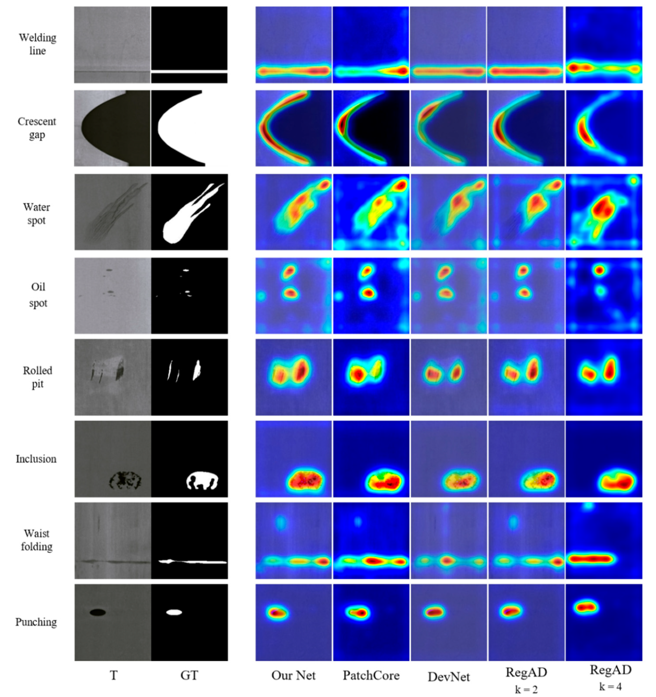
Figure 8 shows the anomaly location visualization results of different advanced methods. The test abnormal image sample image of each category input network is presented in the first column of the graph, and the corresponding pixel-level ground truth maps is presented in the second column of the graph. Other columns present visualization results of different methods. By comparing these visualization results and combining the quantitative results in the previous section, it can be found that the proposed method performs better in the positioning of defects and can deal with the edges and structures of defects more clearly.

4.6. Other Experiments

In addition to experiments on complete datasets, this paper also verifies the performance of anomaly detection methods in small sample scenarios. In order to test the stability of the proposed method when processing small amounts of data, the number of training samples changed from 2 (equivalent to 0.8% of the total training data) to 50 (equivalent to 20% of the total training data), and the same module and training mechanism were used for retraining. Based on the results of the three performance indicators as shown in Figure 9, the proposed method can achieve a certain level of advanced performance even in the case of limited data volume. This shows that the method has strong adaptability. In the actual industrial scene, if the production environment changes, the model only needs to use a small amount of training data for fine-tuning to meet the industrial inspection requirements.

5. Conclusions

In this paper, an anomaly detection model called MKD-IR is proposed, which aims to quickly and accurately screen out abnormal images from a large number of normal strip steel surface images. The MKD-IR model is trained only with normal data. In the test phase, the normal or abnormal images are distinguished by comparing the features of the test set with the features in the stored normal data repository. This method uses a Ms-KD model, which can compress the amount of data computation and make full use of the low-level and high-level information of normal data. In addition, the method also uses the BDCI, which effectively suppresses the tendency of the model to extract natural image data features and improves the sensitivity of the model to abnormal data. Compared with the existing sota method, the proposed method achieves the optimal AUROC and PRO index mean value in the detection of strip surface defects. Through the results of ablation experiments at the same time, we can see the effectiveness of the Ms-KD and BDCI modules.
Meanwhile, a new dataset named SSAD-FSL is proposed in this paper. In general, the method is able to detect anomalies efficiently and accurately in the presence of very complex and diverse anomaly data and can be adapted to the case of insufficient data volume, thus facilitating the development of anomaly detection for strip steel surface defect detection tasks.

Author Contributions

Conceptualization, X.W.; Methodology, W.Z.; Validation, W.Z., Z.Y. and X.W.; Formal analysis, Z.Y. and J.Z.; Investigation, J.Z. and X.W.; Resources, K.S.; Data curation, K.S.; Writing—original draft preparation, X.W., W.Z., Z.Y., J.Z. and K.S.; Writing—review and editing, X.W., W.Z., Z.Y., J.Z. and K.S.; Visualization, Z.Y. and J.Z.; Supervision, K.S.; Project administration, X.W.; Funding acquisition, X.W. All authors have read and agreed to the published version of the manuscript.

Funding

This research was funded by Liaoning Provincial Department of Education Scientific Research Project, grant number LQGD2020023.

Institutional Review Board Statement

Not applicable.

Informed Consent Statement

Not applicable.

Data Availability Statement

Not applicable.

Conflicts of Interest

The authors declare no conflict of interest.

References

  1. He, Y.; Wen, X.; Xu, J. A Semi-Supervised Inspection Approach of Textured Surface Defects under Limited Labeled Samples. Coatings 2022, 12, 1707. [Google Scholar] [CrossRef]
  2. Wen, X.; Shan, J.; He, Y.; Song, K. Steel Surface Defect Recognition: A Survey. Coatings 2022, 13, 17. [Google Scholar] [CrossRef]
  3. Wan, C.; Ma, S.; Song, K. TSSTNet: A Two-Stream Swin Transformer Network for Salient Object Detection of No-Service Rail Surface Defects. Coatings 2022, 12, 1730. [Google Scholar] [CrossRef]
  4. Wang, Y.; Gao, L.; Gao, Y.; Li, X. A new graph-based semi-supervised method for surface defect classification, Robot. Comput. Integr. Manuf. 2021, 68, 102083. [Google Scholar] [CrossRef]
  5. Wang, Y.; Song, K.; Liu, J.; Dong, H.; Jiang, P. RENet: Rectangular convolution pyramid and edge enhancement network for salient object detection of pavement cracks. Measurement 2020, 170, 108698. [Google Scholar] [CrossRef]
  6. Gao, J.; Yuan, D.; Tong, Z.; Yang, J.; Yu, D. Autonomous pavement distress detection using ground penetrating radar and region-based deep learning. Measurement 2020, 164, 108077. [Google Scholar] [CrossRef]
  7. Li, Y.; Wang, H.; Dang, L.M.; Piran, M.; Moon, H. A robust instance segmentation framework for underground sewer defect detection. Measurement 2022, 190, 110727. [Google Scholar] [CrossRef]
  8. Xu, Y.; Li, D.; Xie, Q.; Wu, Q.; Wang, J. Automatic defect detection and segmentation of tunnel surface using modified Mask R-CNN. Measurement 2021, 178, 109316. [Google Scholar] [CrossRef]
  9. Shu, Y.; Li, B.; Li, X.; Xiong, C.; Cao, S.; Wen, X. Deep learning-based fast recognition of commutator surface defects. Measurement 2021, 178, 109324. [Google Scholar] [CrossRef]
  10. Yang, J.; Yang, G. Modified convolutional neural network based on dropout and the stochastic gradient descent optimizer. Algorithms 2018, 11, 28. [Google Scholar] [CrossRef] [Green Version]
  11. Park, J.; Yi, D.; Ji, S. Analysis of recurrent neural network and predictions. Symmetry 2020, 12, 615. [Google Scholar] [CrossRef]
  12. Creswell, A.; White, T.; Dumoulin, V.; Arulkumaran, K.; Sengupta, B.; Bharath, A.A. Generative adversarial networks: An overview. IEEE Signal Process. Mag. 2018, 35, 53–65. [Google Scholar] [CrossRef] [Green Version]
  13. Saberironaghi, A.; Ren, J.; El-Gindy, M. Defect detection methods for industrial products using deep learning techniques: A review. Algorithms 2023, 16, 95. [Google Scholar] [CrossRef]
  14. Elhanashi, A.; Lowe, D.; Saponara, S.; Moshfeghi, Y. Deep Learning Techniques to Identify and Classify COVID-19 Abnormalities on Chest X-ray Images. In Real-Time Image Processing and Deep Learning 2022; SPIE The International Society for Optical Engineering: Bellingham, WA, USA, 2022; Volume 12102, pp. 15–24. [Google Scholar]
  15. Reed, I.S.; Yu, X. Adaptive multiple-band CFAR detection of an optical pattern with unknown spectral distribution. IEEE Trans. Acoust. Speech Signal Process 1990, 38, 1760–1770. [Google Scholar] [CrossRef]
  16. Ester, M.; Kriegel, H.-P.; Sander, J.; Xu, X.W. A Density-Based Algorithm for Discovering Clusters in Large Spatial Databases with Noise. In Proceedings of the Second International Conference on Knowledge Discovery and Data Mining (KDD-96), Portland, OR, USA, 2–4 August 1996; AAAI Press: Washington, DC, USA, 1996; pp. 226–231. [Google Scholar]
  17. Ruff, L.; Vandermeulen, R.; Goernitz, N.; Deecke, L.; Siddiqui, S.; Binder, A.; Muller, E.; Kloft, M. Deep One-Class Classification. In Proceedings of the 35th International Conference on Machine Learning PMLR, Stockholm, Sweden, 10–15 July 2018; pp. 4390–4399. [Google Scholar]
  18. Gao, Y.; Xu, J.; Zhu, X. A novel anomaly detection method based on improved k-means clustering algorithm. J. Ambient. Intell. Humaniz. Comput. 2020, 11, 4223–4233. [Google Scholar]
  19. Oza, P.; Patel, V.M. One-class convolutional neural network. IEEE Signal Process. Lett. 2019, 26, 277–281. [Google Scholar] [CrossRef] [Green Version]
  20. Hendrycks, D.; Mazeika, M.; Dietterich, T.G. Deep Anomaly Detection with Outlier Exposure. In Proceedings of the 7th International Conference on Learning Representations (ICLR), New Orleans, LA, USA, 6–9 May 2019. [Google Scholar]
  21. Goyal, S.; Raghunathan, A.; Jain, M.; Simhadri, H.; Jain, P. DROCC: Deep Robust One-Class Classification. In Proceedings of the 37th International Conference on Machine Learning (PMLR), Virtual, 13–18 July 2020; pp. 3711–3721. [Google Scholar]
  22. Wang, J.Z.; Li, Q.Y.; Gan, J.R.; Yu, H.M.; Yang, X. Surface defect detection via entity sparsity pursuit with intrinsic priors. IEEE Trans. Ind. Inform. 2020, 16, 141–1501. [Google Scholar] [CrossRef]
  23. Gong, D.; Liu, L.; Le, V.; Saha, B.; Mansour, M.; Venkatesh, S.; Hengel, A. Memorizing Normality to Detect Anomaly: Memory-Augmented Deep Autoencoder for Unsupervised Anomaly Detection. In Proceedings of the IEEE/CVF International Conference on Computer Vision, Seoul, Republic of Korea, 27 October–2 November 2019; IEEE Publishing: New York, NY, USA, 2019; pp. 1705–1714. [Google Scholar]
  24. Akcay, S.; Atapour-Abarghouei, A.; Breckon, T.P. Ganomaly: Semi-Supervised Anomaly Detection via Adversarial Training. In Proceedings of the Asian Conference on Computer Vision, Perth, Australia, 2–6 December 2018; Springer: Cham, Switzerland, 2018; pp. 622–637. [Google Scholar]
  25. Schlegl, T.; Seebock, P.; M.Waldstein, S.; Schmidt-Erfurth, U.; Langs, G. Unsupervised Anomaly Detection with Generative Adversarial Networks to Guide Marker Discover. In Proceedings of the International Conference on Information Processing in Medical Imaging, Boone, NC, USA, 25–30 June 2017; Springer: Cham, Switzerland, 2017; pp. 146–157. [Google Scholar]
  26. Perera, P.; Nallapati, R.; Xiang, B. Ocgan: One-Class Novelty Detection Using Gans with Constrained Latent Representations. In Proceedings of the IEEE/CVF Conference on Computer Vision and Pattern Recognition, Long Beach, CA, USA, 16–20 June 2019; pp. 2898–2906. [Google Scholar]
  27. Feng, H.; Song, K.; Cui, W.; Zhang, Y.; Yan, Y. Cross Position Aggregation Network for Few-shot Strip Steel Surface Defect Segmentation. IEEE Trans. Instrum. Meas. 2023, 72, 5007410. [Google Scholar] [CrossRef]
  28. Xiong, L.; Póczos, B.; Schneider, J. Group anomaly detection using flexible genre models. Adv. Neural Inf. Process. Syst. 2011, 24, 1071–1079. [Google Scholar]
  29. Laurence, W.; Nemhauser, G. Integer and Combinatorial Optimization; Wiley: Hoboken, NJ, USA, 2014. [Google Scholar]
  30. Dasgupta, S.; Gupta, A. An elementary proof of a theorem of Johnson and Lindenstrauss. Random Struct. Algorithms 2003, 22, 60–65. [Google Scholar] [CrossRef]
  31. Song, K.; Yan, Y. A noise robust method based on completed local binary patterns for hot-rolled steel strip surface defects. Appl. Surf. Sci. 2013, 285, 858–864. [Google Scholar] [CrossRef]
  32. Feng, X.; Gao, X.; Luo, L. X-SDD: A new benchmark for hot rolled steel strip surface defects setection. Symmetry 2021, 13, 706. [Google Scholar] [CrossRef]
  33. Lv, X.; Duan, F.; Jiang, J.J.; Fu, X.; Gan, L. Deep metallic surface defect detection: The new benchmark and detection network. Sensors 2020, 20, 1562. [Google Scholar] [CrossRef] [PubMed] [Green Version]
  34. Roth, K.; Pemula, L.; Zepeda, J.; Scholkopf, B.; Brox, T.; Gehler, P. Towards Total Recall in Industrial Anomaly Detection. In Proceedings of the IEEE/CVF Conference on Computer Vision and Pattern Recognition, New Orleans, LA, USA, 18–24 June 2022; pp. 14318–14328. [Google Scholar]
  35. Pang, G.; Shen, C.; van den Hengel, A. Deep Anomaly Detection with Deviation Networks. In Proceedings of the 25th ACM SIGKDD International Conference on Knowledge Discovery & Data Mining, Anchorage, AK, USA, 4–8 August 2019; Association for Computing Machinery: New York, NY, USA, 2019; pp. 353–362. [Google Scholar]
  36. Huang, C.; Guan, H.; Jiang, A.; Zhang, Y.; Spratling, M.; Wang, Y.-F. Registration Based Few-Shot Anomaly Detection Computer Vision–ECCV 2022. In Proceedings of the 17th European Conference, Tel Aviv, Israel, 23–27 October 2022; Springer Nature: Cham, Switzerland, 2022; pp. 303–319. [Google Scholar]
  37. Sheynin, S.; Benaim, S.; Wolf, L. A hierarchical Transformation-Discriminating Generative Model for Few Shot Anomaly Detection. In Proceedings of the IEEE/CVF International Conference on Computer Vision, Montreal, BC, Canada, 11–17 October 2021; pp. 8495–8504. [Google Scholar]
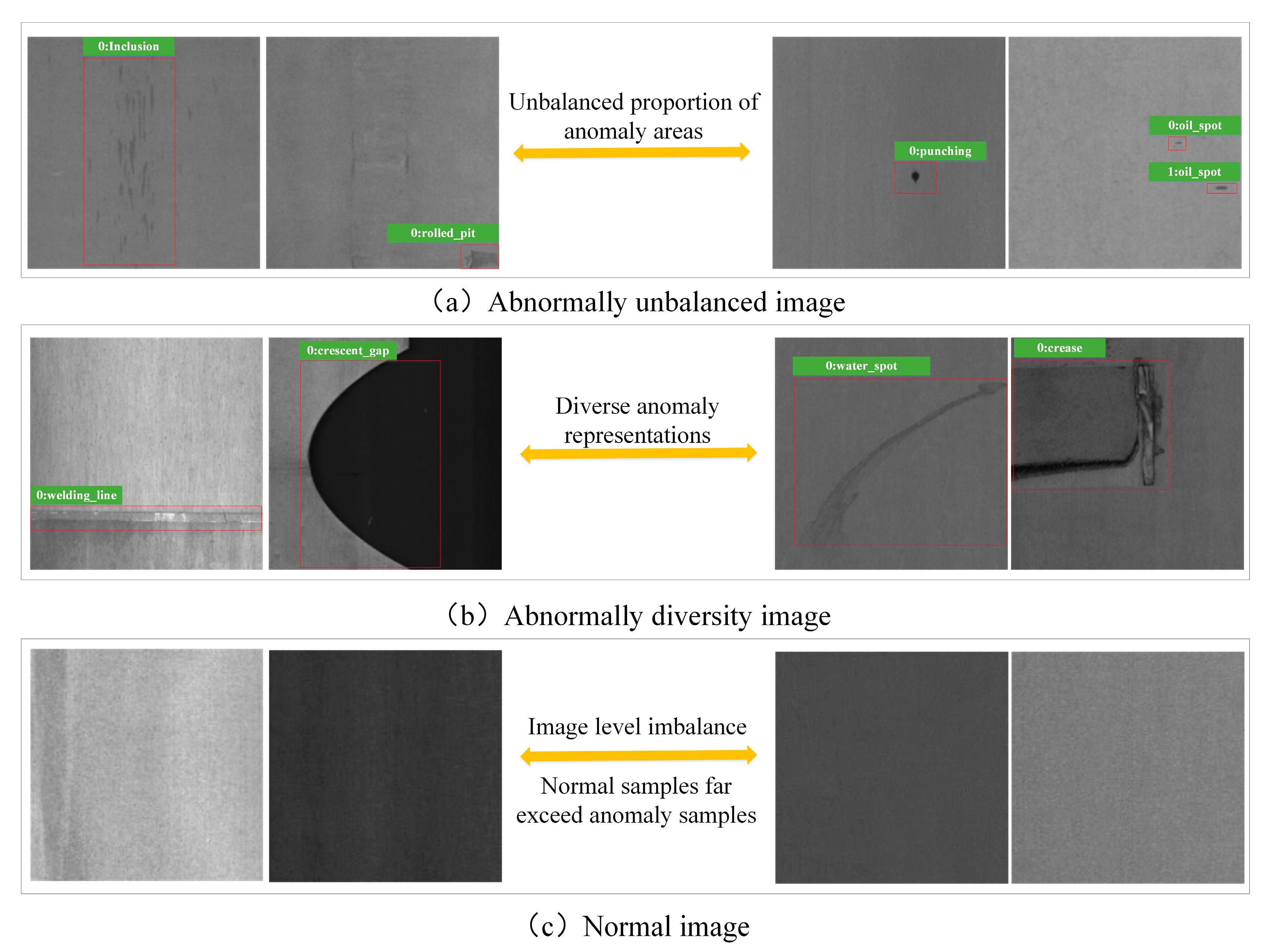
Figure 1. Difficulties in detecting strip anomalies.
Coatings 13 01171 g001
Figure 2. Structure of the MKD-IR model.
Coatings 13 01171 g002
Figure 3. Multi-scale knowledge distillation module.
Coatings 13 01171 g003
Figure 4. The diagram for obtaining anomaly scores.
Coatings 13 01171 g004
Figure 5. Schematic diagram of part of the SSAD-FSL defective dataset. The first row of the image shows the defect image, and the second row shows the pixel level truth image corresponding to the defect image.
Coatings 13 01171 g005
Figure 6. Comparative experiment curves. (a) ROC Curve. (b) PR Curve.
Coatings 13 01171 g006
Figure 7. The quantitative results of distillation simplified model or same model.
Coatings 13 01171 g007
Figure 8. Visualization comparison results on SSAD-FSL dataset.
Coatings 13 01171 g008
Figure 9. Results of few shot experiments on SSAD-FSL dataset.
Coatings 13 01171 g009
Table 1. Comparison of anomaly detection techniques under different methods.
CategoryModelRef.AdvantagesDisadvantages
Anomaly detection method based on distance measureOne-class convolutional neural network[17]Support vector machine is applied to surface defect detection tasksMethods are not effective for complex datasets and are prone to model degradation
Deep anomaly detection with outlier exposure[18]Support vector machine is applied to surface defect detection tasksMethods are not effective for complex datasets and are prone to model degradation
Anomaly detection method based on constructing classification surfaceSurface defect detection via entity sparsity pursuit with intrinsic priors[20]Flexibly handle complex data distributionComplex
Anomaly detection method based on image reconstructionMemorizing normality to detect anomaly[21]Improving the performance of classification and clusteringPoor performance in some real datasets
Unsupervised anomaly detection with generative adversarial networks to guide marker discovery[23]The reconstructed image has integrityThe dimension of the hidden variable relative to the dimension of the generated image will cause its effect to change
One-class novelty detection using gans with constrained latent representations[24]Uniform vector distributionThe robustness of this model is not good
Table 2. The quantitative results of image level AUROC comparisons on the SSAD-FSL dataset.
Defect TypePatchCoreDevNetRegADHTDGOurNet
Batch Size 32 k = 2Batch Size 16 k = 4Without
Norm
With
T1 Norm
Welding line0.98530.98580.81260.87540.87530.88470.9753
Crescent gap11110.8930 0.89291
Water spot10.96550.85140.88480.80120.80121
Oil spot0.94060.94950.92670.96190.83880.8400 0.9506
Rolled pit0.97510.9460 0.92440.95190.83760.83650.9741
Inclusion110.94820.98040.78120.78121
Waist folding0.94650.98930.91730.95350.95050.95060.9941
Punching11110.97870.97861
Average 0.9809 0.9795 0.9226 0.9510 0.8695 0.8707 0.9868
Table 3. The quantitative results of pixel-level AUROC comparisons on the SSAD-FSL dataset.
Defect TypePatchCoreDevNetRegADHTDGOurNet
Batch Size 32 k = 2Batch Size 16 k = 4
Welding line0.8290 0.8030 0.68330.7435\0.9195
Crescent gap0.91930.59120.9930 0.9876\0.9585
Water spot0.75510.65110.66640.6892\0.7419
Oil spot0.87340.76560.75250.7554\0.7791
Rolled pit0.90190.86010.72670.7964\0.8822
Inclusion0.90690.92950.7495 0.7058\0.9478
Waist folding0.8483 0.65040.7375 0.7661\0.9172
Punching0.99560.9210 0.73570.7795\0.9932
Average 0.8787 0.7715 0.7556 0.7779 \0.8924
Table 4. The quantitative results of pixel-level PRO comparisons on the SSAD-FSL dataset.
Defect TypePatchCoreDevNetRegADHTDGOurNet
Batch Size 32 k = 2Batch Size 16 k = 4
Welding line0.92120.97460.91990.9497\0.9764
Crescent gap1111\1
Water spot0.96780.99370.91070.9406\0.9902
Oil spot0.97580.96830.97150.9838\0.9673
Rolled pit0.98470.97890.96320.9767\0.9951
Inclusion110.9880 0.9919\1
Waist folding0.97980.99770.9660 0.9812\0.9874
Punching1111\1
Average 0.9787 0.9892 0.9649 0.9780 \0.9896
Table 5. The quantitative results of ablation experiment.
Ms-KDBDCIImg-AUROCPixel-AUROCPRO
0.95870.87670.9654
0.96650.88420.9733
0.98680.89240.9896
Table 6. The quantitative results of ablation experiments with different loss functions.
TypeWelding LineCrescent GapWater SpotOil SpotRolled PitInclusionWaist FoldingPunchingAverage
LMID(first three layers)0.9453 0.9600 0.9535 0.9434 0.9412 0.9500 0.9621 0.9574 0.9516
LMID(last three layers)0.9465 0.9800 0.9738 0.9258 0.9600 0.9467 0.9870 0.9628 0.9603
Llast layer0.9589 0.9841 0.9924 0.9558 0.9587 0.9600 0.9697 0.9710 0.9688
LALL0.9753 1.0000 1.0000 0.9506 0.9741 1.0000 0.9941 1.0000 0.9868
Disclaimer/Publisher’s Note: The statements, opinions and data contained in all publications are solely those of the individual author(s) and contributor(s) and not of MDPI and/or the editor(s). MDPI and/or the editor(s) disclaim responsibility for any injury to people or property resulting from any ideas, methods, instructions or products referred to in the content.