Automated Crack Detection in 2D Hexagonal Boron Nitride Coatings Using Machine Learning

Abstract

Characterizing defects in 2D materials, such as cracks in chemical vapor deposited (CVD)-grown hexagonal boron nitride (hBN), is essential for evaluating material quality and reliability. Traditional characterization methods are often time-consuming and subjective and can be hindered by the limited optical contrast of hBN. To address this, we utilized a YOLOv8n deep learning model for automated crack detection in transferred CVD-grown hBN films, using MATLAB’s Image Labeler and Supervisely for meticulous annotation and training. The model demonstrates promising crack-detection capabilities, accurately identifying cracks of varying sizes and complexities, with loss curve analysis revealing progressive learning. However, a trade-off between precision and recall highlights the need for further refinement, particularly in distinguishing fine cracks from multilayer hBN regions. This study demonstrates the potential of ML-based approaches to streamline 2D material characterization and accelerate their integration into advanced devices.

1. Introduction

Two-dimensional (2D) materials possess a unique set of properties due to their reduced dimensionality, making them promising candidates for replacing traditional materials in cutting-edge electronics, photonics, and nanoelectromechanical systems [1]. Hexagonal boron nitride (hBN) is a promising dielectric material due to its wide bandgap (>5 eV), high transparency, and unique mechanical properties [2,3,4]. Its broad range of applications spans optoelectronics, solid-state neutron detectors, field-effect transistors, tunneling devices, electron emitters, deep UV emitters, photonic devices, switching/memory devices, super capacitors, and environmental monitoring [5,6,7,8]. The ability to fabricate heterostructures with tailored properties further amplifies the potential of hBN and other 2D materials [9,10]. Notably, hBN serves as a complementary 2D substrate for graphene-based electronics, enhancing their performance [11,12]. In these heterostructures, hBN plays a crucial role by encapsulating other 2D materials like graphene, thereby improving their performance and enabling the study of new physical phenomena [13,14].

Chemical vapor deposition (CVD) has emerged as the most suitable technique for synthesizing atomically thin hBN films and heterostructures on a large scale while maintaining material quality. The CVD technique is deployed to synthesize hBN films onto various metallic substrates, including Cu, Ni, and Pt [2,15,16,17,18,19]. The fabrication and characterization of devices based on 2D materials frequently necessitate the use of non-metal substrates, which in turn involve a variety of transfer techniques to move the synthesized materials from the growth substrate to the desired target substrate. CVD growth followed by wet-etch transfer methods enable the integration of large-area, high-quality hBN films into advanced electronic devices, such as dielectric layers for graphene devices, field-effect transistors, and thermoelectric devices [3,12,16,20].

However, the wet transfer process can introduce defects such as cracks, wrinkles, and polymer residues, which can significantly degrade the material’s properties and hinder its performance in devices [21]. Cracks, in particular, can severely compromise mechanical strength, hBN’s barrier properties, and introduce charge scattering sites [22,23,24]. These cracks may arise from stresses during transfer or from bubbles formed during the etching process that induce strain upon the film [25]. Current crack-detection methods relying on manual inspection and sophisticated characterization tools are time-consuming and costly. These methods are prone to human error, especially with large-area samples or high-throughput production. While wrinkles and polymer residues present their own challenges, this study focuses specifically on automating the detection of cracks in transferred CVD-grown hBN films, as addressing crack identification holds immediate value for quality control and accelerating the integration of hBN into advanced devices. The limitations of current crack-detection methods highlight the need for an automated, rapid, and cost-effective approach to enable efficient quality control and facilitate the widespread adoption of hBN in advanced electronic devices.

To fully harness the potential of hBN and other 2D materials, efficient and reliable characterization techniques are essential. However, the large-scale characterization of 2D materials remains a challenge due to the complexity of traditional methods. Their atomic-level thinness demands specialized techniques that can be intricate and time-consuming [26]. The lack of standardized characterization protocols further hinders the comparison of results across studies. Moreover, 2D materials are highly sensitive to defects, the underlying substrate, and their interfaces with other materials, making consistent characterization even more difficult [27].

Traditional characterization techniques often involve laborious manual assessment and rely heavily on domain expertise, leading to potential subjectivity, errors, and slow analysis. Optical microscopy, though a common initial tool due to its speed, accessibility, and non-destructive nature, has limitations [28]. These include resolution constraints, difficulty in providing precise quantitative information, and sensitivity to external factors like the substrate, which can complicate the analysis of 2D materials [29]. Unlike graphene, hBN’s wide bandgap results in low optical contrast, especially on standard SiO₂ substrates. Additionally, the contrast fluctuates across the visible spectrum, with a near-zero value in the green region, where the human eye is most sensitive [30]. Hence hBN characterization requires more time and domain expertise. To overcome these limitations and accelerate hBN’s widespread adoption, we introduce a machine learning approach capable of rapid and automated crack detection in CVD-grown hBN.

The rapid development of machine learning (ML), along with new algorithms, growing datasets, and increased computational power, is revolutionizing various research areas [31,32,33,34,35,36]. ML is transforming 2D material sciences. By analyzing complex datasets and relationships between properties, ML can streamline characterization efforts that are traditionally time-consuming and require domain expertise. This makes ML particularly valuable for predicting properties, guiding the discovery of novel 2D materials, and optimizing their integration into cutting-edge applications [37]. Importantly, ML accelerates the development of 2D materials by streamlining data collection, analysis, and the exploration of structure–property relationships. This overcomes the limitations of traditional methods that often rely on extensive, time-consuming experiments, ultimately leading to the discovery of new materials and tailored optimization for specialized applications [38,39].

While ML applications in 2D materials’ optical characterization are still evolving, much of the existing work centers on graphene and exfoliated samples, primarily focusing on distinguishing graphene flakes’ thickness and identifying different 2D material flakes and their heterostructures [40,41,42,43,44,45,46,47]. Ramezani et al. [48] focused on identifying exfoliated hBN flakes via deep learning, while our previous study [49] utilized unsupervised models to distinguish multilayer hBN regions. While these models have shown promise, their original designs may not be ideal for identifying hBN crack morphologies, especially those found in CVD-grown hBN due to diverse crack morphologies from transfer processes, substrate effects, and potential interference from other defects like wrinkles or residues. ML-based analysis has been applied in multiple instances to identify point defects in 2D materials, but these defect identification methods require sophisticated tools, such as transmission electron microscopy (TEM) [50,51,52].

Our study shifts the focus specifically to hBN, particularly addressing the growing use of large-area CVD synthesis in the production of 2D materials [2,15,16]. With successful large-area transfer techniques to arbitrary substrates [53,54], our research aims to tackle the bottleneck of efficient large-area characterization of these transferred CVD-grown hBN samples. By developing an ML-based approach, we strive to streamline this process and facilitate the widespread application of hBN.

To address this challenge of crack detection in CVD-grown hBN, this study utilizes the power of YOLOv8n deep learning models. Our proposed algorithm can process optical microscope images with a resolution of 1024 × 768 pixels in just 291 ms, enabling the real-time detection of cracks in hBN films. To the best of our knowledge, this study is among the first to apply ML for crack identification in transferred CVD-grown hBN samples. This work has the potential to streamline quality control and accelerate the use of hBN in advanced devices.

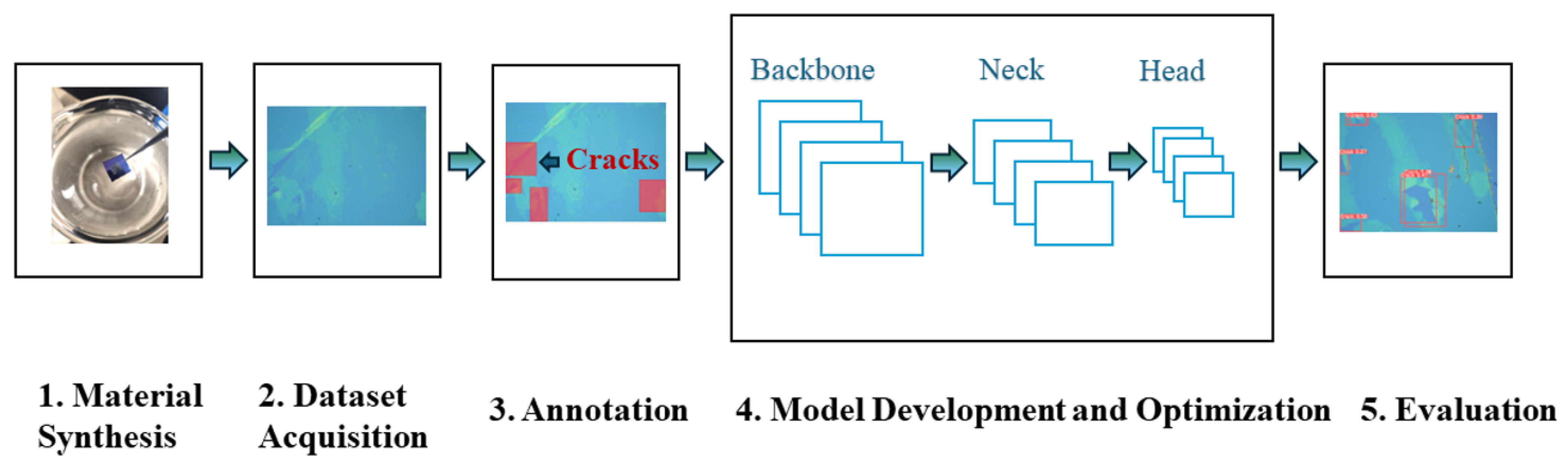
2. Materials and Methods

Having highlighted the limitations of traditional hBN crack detection and the promise of machine learning, we now present a comprehensive methodology designed to address these challenges. This section presents an integrated workflow, encompassing material synthesis, dataset acquisition, annotation, model development and optimization, and evaluation. Our solution, outlined in Figure 1, leverages the power of the YOLOv8n object detection model to accurately identify crack regions within transferred CVD-grown hBN samples. The following subsections provide detailed insights into each stage of the process, from sample preparation and data collection to model training, tuning, and performance assessment.

2.1. Material Synthesis

To investigate crack detection in CVD-grown hBN, a well-established PMMA-assisted wet-etch transfer method was utilized for sample preparation [15,53,55,56]. A Multilayer hBN on copper foil (SKU: CVD-2X1-BN-ML) was obtained from Graphene Laboratories Inc. (Ronkonkoma, NY, USA). The films were transferred onto 500 $\mu$m thick doped p-type silicon wafers (<0.01$\Omega$-cm) with a 300 nm SiO₂ layer (ACS material). This choice of substrate provided suitable optical contrast for subsequent imaging.

For sample preparation, a PMMA solution (4.5% in anisole) was spin-coated onto 1 × 1 cm² hBN/Cu foil sections at 2500 rpm for 1 min to create a protective layer. The PMMA/hBN/Cu samples were then placed on a 0.15–0.2 M potassium persulfate etchant solution to dissolve the copper foil, leaving the PMMA/hBN film floating. Thorough rinsing with DI water (5 min per cycle, repeated three times) removed residual etchant. The floating PMMA/hBN film was carefully transferred to a prepared Si/SiO₂ substrate (1.5 × 1.5 cm²). Air-drying for 30 min and heating at 100 °C for 20 min promoted adhesion before the PMMA layer was dissolved in acetone. Finally, the sample was immersed in acetone for 30 min to dissolve the PMMA layer, leaving the hBN film on the Si/SiO₂ substrate. This process yielded a total of 10 multilayer hBN samples for subsequent characterization and analysis.

2.2. Dataset Acquisition

To build the image dataset, a VK-X250 laser confocal scanning microscope (CLSM) (Keyence Corp, Itasca, IL, USA) with a 10× objective was used to capture optical images of the transferred hBN films. A total of 150 images were collected, specifically focused on MLhBN regions. To ensure consistency and comparability within the dataset, uniform camera settings, image size, and intensity were maintained during the acquisition process. Images were initially acquired in VK4 file format and then converted to the widely compatible PNG format using the multi-file analysis application (VK-H1XME) software. This conversion preserved the high resolution for subsequent analysis. All images have a final size of 1.4 mm × 1 mm.

2.3. Annotation

Careful data preprocessing and labeling are crucial for developing accurate supervised models. MATLAB R2023b’s Image Labeler was employed to meticulously annotate images, defining regions of interest for ground truth comparison. The annotated images were saved in both MATLAB project file and JSON formats for flexibility. To further refine the annotations, the Supervisely platform was utilized. For robust model evaluation, the dataset was strategically divided into two groups:

• Training Set (92 images): The core dataset used to train the machine learning model.
• Validation Set (24 images): Used to optimize model hyperparameters.

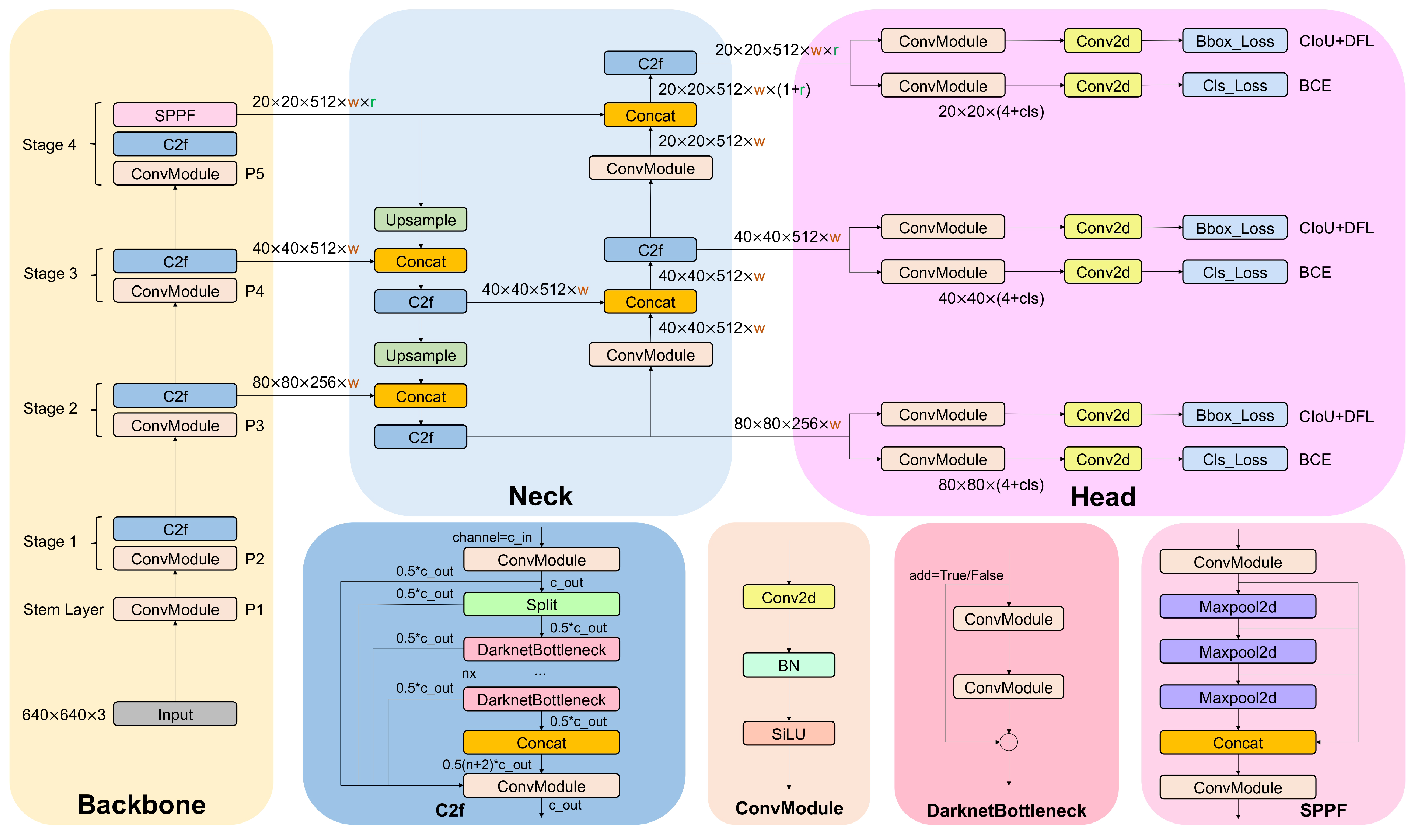
2.4. Model Development and Optimization

Fine-tuning was employed on the pre-trained YOLOv8n-det model provided by Ultralytics to detect crack regions within the datasets [57]. The YOLOv8 architecture represents a series of enhancements and extensions introduced by Ultralytics to the YOLOv5 framework. These improvements primarily focus on scaling adjustments and architectural refinements, aiming to augment the model’s performance and capabilities. The architecture consists of three major parts: backbone, neck, and head.

2.4.1. Backbone

The backbone layer is composed of a series of convolutional neural networks (CNNs) trained more effectively with reduced computational cost using the Cross-Stage Partial (CSP) architecture design [58]. The model uses a C2f module consisting of 2 ConvModule and n DarknetBottleneck allowing the model to collect richer gradient flow information. The ConvModule consists of Conv-BN-SiLU, and n is the number of bottlenecks, as shown in Figure 2. Additionally, the model adopts the Spatial Pyramid Pooling–Fast (SPPF) module, allowing an improved inference speed of the model.

2.4.2. Neck

Typically, networks with more layers are able to extract a greater range of feature information, which can enhance the quality of dense predictions. Yet, when networks become overly deep, they may start to lose crucial spatial details of objects, particularly if there are excessive convolution operations, which could lead to a loss of information about smaller objects. To mitigate this, it is beneficial to employ Feature Pyramid Network (FPN) [60] and Path Aggregation Network (PAN) [61], which enable the fusion of features across multiple scales. As depicted in Figure 2, the neck component of the architecture integrates features from various network levels. This process enriches the feature information in the higher levels thanks to additional layers, while the initial layers retain more spatial details due to having undergone fewer convolutions.

2.4.3. Head

The model features a decoupled head, separating the processes of classification and detection into distinct components. The architecture simplifies this by maintaining only the branches for classification and regression. Unlike techniques that use a predefined set of anchors to ascertain object locations by calculating offsets, this model implements an anchor-free method. This method locates the center of the object and gauges the distances to the edges of the bounding box, thereby refining the prediction of the object’s location without relying on anchors.

2.4.4. Loss

The YOLOv8 algorithm employs the Task-Aligned Assigner from TOOD [62] for designating both negative and positive samples. It selects positive samples by considering a combination of weighted scores from both classification and regression, as delineated in the subsequent equation.

$$t=s^{\alpha }\times u^{\beta }$$

(1)

where s is the predicted score for the given class label, and u signifies the Intersection over Union (IoU) between the predicted and actual bounding boxes.

The model comprises separate classification and regression branches. For classification, Binary Cross-Entropy (BCE) Loss is used, as shown in the following equation:

$${\mathrm{Loss}}_{\mathrm{cls}}=-w[y_{n}log{x}_n+(1-y_n)log(1-x_n)]$$

(2)

where w represents the weight, $y_n$ is the true label, and $x_n$ is the model’s predicted value.

For regression, the model applies Distributed Focal Loss (DFL) and Complete IoU (CIoU) Loss. The DFL is aimed at refining the probability distribution around the object y:

$$\mathrm{DFL}\left({\mathcal{S}}_n,{\mathcal{S}}_{n+1}\right)=-\left[(y_{n+1}-y)log\left({\mathcal{S}}_n\right)+(y-y_n)log\left({\mathcal{S}}_{n+1}\right)\right]$$

(3)

where ${\mathcal{S}}_n$ and ${\mathcal{S}}_{n+1}$ are probabilities for the ground truth and are computed as

$${\mathcal{S}}_n=\frac{y_{n+1}-y}{y_{n+1}-y_n},{\mathcal{S}}_{n+1}=\frac{y-y_n}{y_{n+1}-y_n}$$

(4)

CIoU Loss integrates an additional term to account for the aspect ratio of the bounding boxes [59]:

$$CIo{U}_{Loss}=1-IoU+\frac{Distanc{e}^2}{Distanc{e}_c^2}+\frac{{\nu }^2}{(1-IoU)+\nu }$$

(5)

with $\nu$ as the measure of aspect ratio consistency, which is defined by

$$\nu =\frac{4}{{\pi }^2}{\left(arctan\frac{w^{gt}}{h^{gt}}-arctan\frac{w^p}{h^p}\right)}^2$$

(6)

Here, w represents the width of bounding box, and h represents the height of the bounding box.

2.4.5. Data Augmentation and Model Optimization

In the course of training the model, the Supervisely platform served as the primary environment. A variety of data augmentation techniques were employed to enhance the robustness and generalizability of the model. These techniques included the following.

(a)

HSV (Hue, Saturation, Value) Augmentation: This method adjusts the color properties of images to simulate a wider range of lighting conditions and object appearances. The transformations can be represented mathematically as

$$H^{\prime }=H+\Delta H,S^{\prime }=S\times (1+\Delta S),V^{\prime }=V\times (1+\Delta V)$$

(7)

where H, S, and V are the original hue, saturation, and value components of the image pixels, respectively. $H^{\prime }$, $S^{\prime }$, and $V^{\prime }$ are the augmented components, and $\Delta H$, $\Delta S$, and $\Delta V$ represent small, random perturbations applied to each channel.

(b)

Translation: This technique shifts the image by a certain number of pixels horizontally and vertically, introducing variability in object positioning within the frame. The translation operation can be described by the transformation matrix:

$$T=\left[\begin{array}{ccc}1& 0& \Delta x\\ 0& 1& \Delta y\\ 0& 0& 1\end{array}\right]$$

(8)

where $\Delta x$ and $\Delta y$ denote the horizontal and vertical displacements, respectively.

(c)

Scaling: Scaling alters the size of the image, simulating objects at different distances from the viewer. This operation can be mathematically represented by the scaling matrix:

$$S=\left[\begin{array}{ccc}\alpha & 0& 0\\ 0& \beta & 0\\ 0& 0& 1\end{array}\right]$$

(9)

where $\alpha$ and $\beta$ are scaling factors for the width and height of the image, respectively.

(d)

Flipping Operations: Flipping operations mirror the image either horizontally, vertically, or both to simulate different orientations of objects. The flipping transformation can be represented as a reflection matrix, for example, for horizontal flipping:

$$F_h=\left[\begin{array}{ccc}-1& 0& W\\ 0& 1& 0\\ 0& 0& 1\end{array}\right]$$

(10)

where W is the width of the image, ensuring the flipped image remains within the original dimensions.

Each of these augmentation techniques introduces variations in the training dataset, thus enabling the model to learn more generalized features and improving its performance on unseen data.

The model was trained over 300 epochs in the fine-tune mode in the Supervisely platform with NVIDIA GeForce RTX 3080 GPU, input image size of 640, and a batch size of 8, employing an SGD optimizer and the hyperparameters detailed in

Table 1. Hyperparameter settings for optimizing the YOLOv8n model’s performance on Supervisely.

Parameter	Value
initial learning rate (lr0)	0.01
final learning rate (lrf)	0.01
Adam beta1 (momentum)	0.937
optimizer weight decay (weight_decay)	0.0005
warmup epochs (warmup_epochs)	3.0
warmup initial momentum	0.8
warmup initial bias lr	0.1
Automatic Mixed Precision (AMP) training	True

. An early stopping technique was employed to select the best weights.

2.5. Evaluation

Precision, recall, a confusion matrix, mAP50, and the mA50-95 score were used to assess the model’s performance during training. Precision measures the reliability of detections, indicating the certainty that an identified crack is indeed a true positive (TP). Conversely, a false positive (FP) occurs when the detector wrongly identifies a crack. Recall measures how well the detector finds true cracks, reflecting its ability to avoid false negatives (FNs) where cracks are missed. These classifications (TP, FP, TN, FN), visualized in the confusion matrix, directly influence the precision and recall scores.

The formulas for precision and recall are defined as follows:

$$\mathrm{Precision}\left(\mathrm{P}\right)=\frac{\mathrm{True}\mathrm{Positives}}{\mathrm{True}\mathrm{Positives}+\mathrm{False}\mathrm{Positives}}$$

(11)

$$\mathrm{Recall}\left(\mathrm{R}\right)=\frac{\mathrm{True}\mathrm{Positives}}{\mathrm{True}\mathrm{Positives}+\mathrm{False}\mathrm{Negatives}}$$

(12)

Confusion matrices provide a comprehensive summary of the model’s predictions compared to ground truth labels. This visual tool facilitates the assessment of accuracy, precision, recall, and other performance metrics.

To provide an even more robust assessment, we extend our evaluation with the mAP50 and mA50-95 scores. mAP50 (mean average precision at IoU 50%) measures the average precision of object detection across different classes at a specific Intersection over Union (IoU) threshold of 50%. IoU quantifies the overlap between the predicted bounding boxes and the ground truth annotations. A higher mAP50 value indicates better localization accuracy and precision of detected cracks, making it particularly useful for evaluating the model’s performance when cracks exhibit varying sizes and shapes.

For a single class, average precision (AP) is the area under the precision–recall curve. mAP50 is computed by taking the mean of the AP values across all classes at an IoU threshold of 50%. The formulas for IoU and AP calculation are as follows:

$$\mathrm{IoU}(A,B)=\frac{\mathrm{area}\mathrm{of}\mathrm{overlap}\mathrm{between}A\mathrm{and}B}{\mathrm{area}\mathrm{of}\mathrm{union}\mathrm{of}A\mathrm{and}B}$$

(13)

$$AP={\int }_0^{1}P\left(R\right)dR$$

(14)

$$mAP50=\frac{1}{N}\sum _{i=1}^{N}A{P}_{50}^i$$

(15)

where N is the number of classes and $A{P}_{50}^i$ is the AP calculated at an IoU threshold of 50% for class i.

The mA50-95 score (mean average precision across different IoU thresholds from 50% to 95%) goes beyond a single IoU threshold. It provides a comprehensive assessment of the model’s performance across a range of IoU values, offering insights into its robustness and generalization ability. A higher mA50-95 score signifies superior detection performance across diverse conditions, indicating the model’s effectiveness in accurately detecting cracks.

The selection of appropriate evaluation metrics is crucial for obtaining a comprehensive understanding of a machine learning model’s performance. This study demonstrates the value of a multi-faceted assessment using precision, recall, confusion matrix, mAP50, and mA50-95 scores. These metrics collectively reveal the model’s reliability in identifying true cracks, its ability to minimize missed detections, and its performance across varying crack characteristics. These insights collectively provide a robust basis for model optimization, ensuring its effectiveness in reliable crack detection for hBN characterization tasks.

3. Results

The following section presents a comprehensive analysis of the proposed YOLOv8n model’s performance in crack-detection tasks. The aim is to assess the model’s strengths, limitations, and learning dynamics through a combination of visual inspection, quantitative metrics, and loss curve analysis.

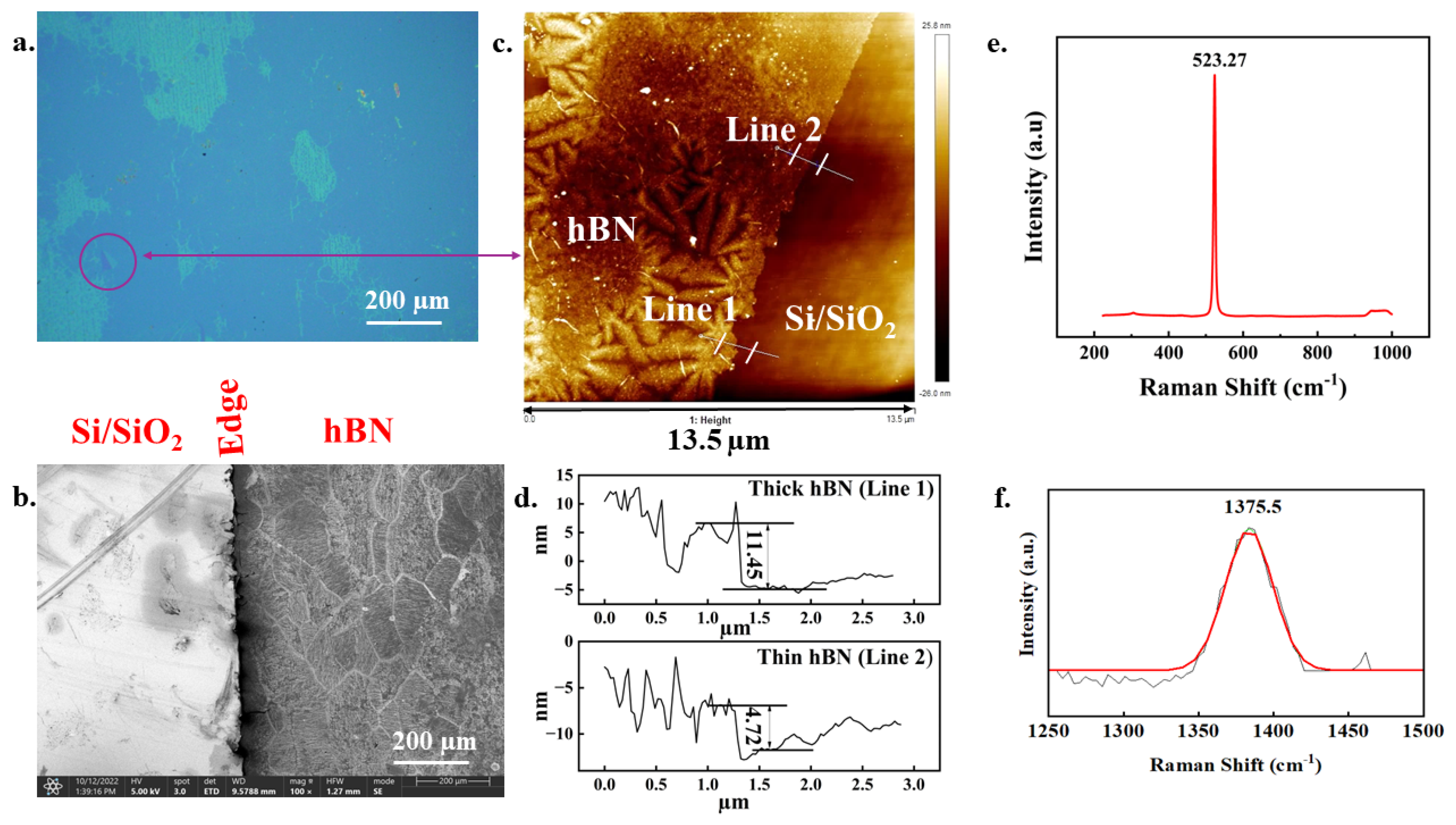
3.1. hBN Film Characterization

Figure 3 provides a comprehensive analysis of multilayer hexagonal boron nitride films transferred on a Si/SiO₂ substrate. Figure 3a shows an optical image of the multilayer hBN sample, while Figure 3b presents a scanning electron microscopy (SEM) image highlighting the edges of the hBN and the underlying Si/SiO₂ topography.

Figure 3c displays an atomic force microscopy (AFM) height image, which zooms in on the region shown in Figure 3a. The line scan profiles obtained from the AFM data are presented in Figure 3d, revealing the presence of two distinct hBN layers with varying thicknesses. The first line, labeled “Line 1”, corresponds to a thick hBN layer with an average thickness of approximately 11.45 nm, while the second line, “Line 2”, represents a thinner hBN layer with an average thickness of 4.72 nm.

To further characterize the sample, Raman spectroscopy measurements were performed. Figure 3e shows the Raman spectrum obtained from the crack regions, where the Si Raman mode is visible due to the absence of the hBN film, serving as a background signal. On the other hand, Figure 3f depicts the Raman spectrum acquired from the film areas. After applying a Voigt fitting procedure, the hBN film Raman shift is found to be 1375.5 cm⁻¹, which aligns with the expected Raman shift for multilayer hBN.

The combination of optical microscopy, SEM, AFM, and the Raman spectroscopy provides a comprehensive understanding of the multilayer hBN sample’s morphology, thickness, and structural properties. The varying thicknesses observed in the AFM line scans, along with the distinct Raman signatures from the crack and film regions, offer valuable insights into the quality and uniformity of the transferred hBN films. These characteristics highlight the challenges for crack detection. Having characterized the hBN film’s properties and potential defects, let us now analyze the model’s performance in specifically identifying cracks within this sample.

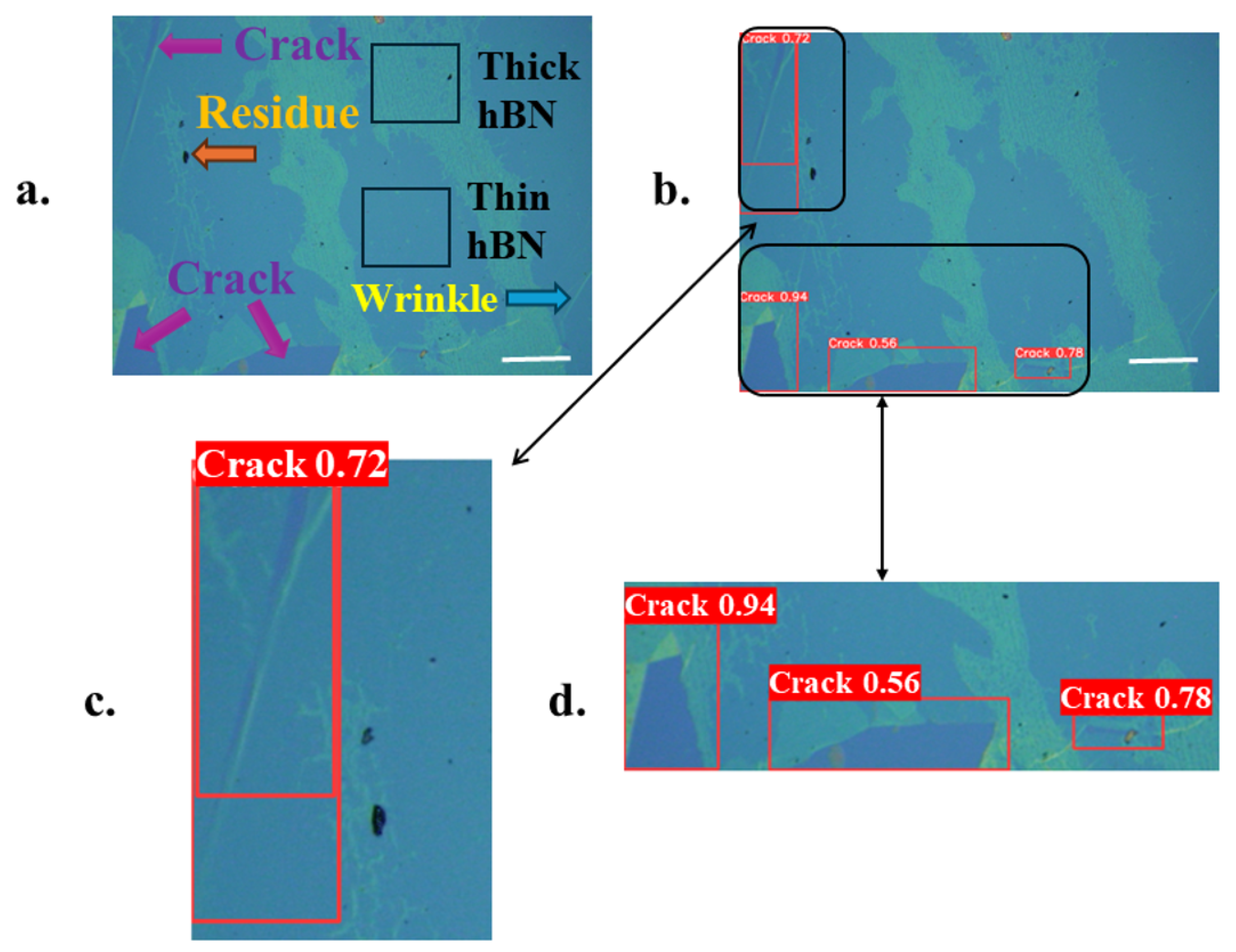
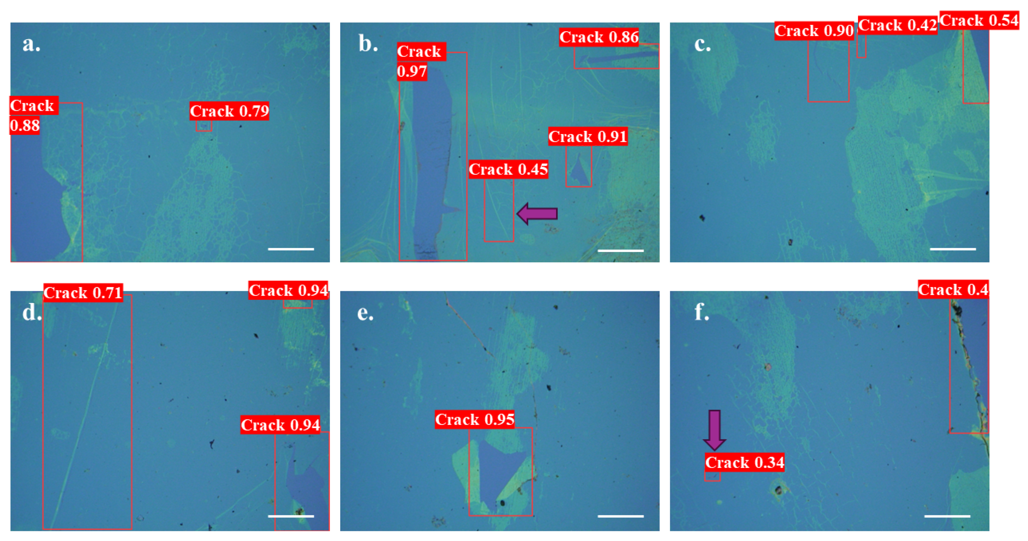
3.2. Visualizing Model Performance: Qualitative Analysis of Crack Detection

Figure 4 demonstrates the YOLOv8n model’s promising capabilities in crack detection. In the raw image shown in Figure 4a, the color contrast highlights various defects and hBN characteristics. Cracks appear distinctively as dark blue regions (purple arrows), while black regions (orange arrow) suggest the presence of residue, and brighter blue lines indicate wrinkles. Color variations also reveal thick (brighter) and thin hBN (lighter blue) areas. The model successfully identifies multiple cracks in Figure 4b, assigning bounding boxes and confidence scores. The zoomed-in views in Figure 4c,d demonstrate its ability to accurately identify both single and intersecting cracks, even those with finer details. This robust performance against variations in crack size, orientation, clarity, and background complexity offers initial evidence of the model’s potential for automated hBN characterization.

A more comprehensive picture of the model’s strengths and weaknesses emerges in Figure 5. Notably, the model accurately detects and precisely bounds cracks of varying sizes Figure 5a–f. Its ability to successfully localize even intersecting cracks (Figure 5c) further demonstrates its capabilities. Confidence scores associated with each prediction add a valuable dimension to the analysis, particularly aligning with the model’s certainty.

However, limitations also exist. In some cases, the model misidentifies background MLhBN regions as cracks (particularly fine or low-contrast ones), leading to false positives (purple arrows in Figure 5b,f). Additionally, the precision of bounding boxes occasionally suffers, likely due to challenges in accurately outlining irregular crack patterns. Further refinement could address the observed variability in confidence scores assigned to similar-looking cracks, potentially improving robustness and reducing biases within the model’s decision-making process.

These results demonstrate the model’s promising ability to detect cracks of various types, but also highlight a need to refine its precision for fine cracks and complex crack patterns. A deeper analysis of the model’s errors and decision-making, as revealed through quantitative metrics, will shed further light on areas for improvement.

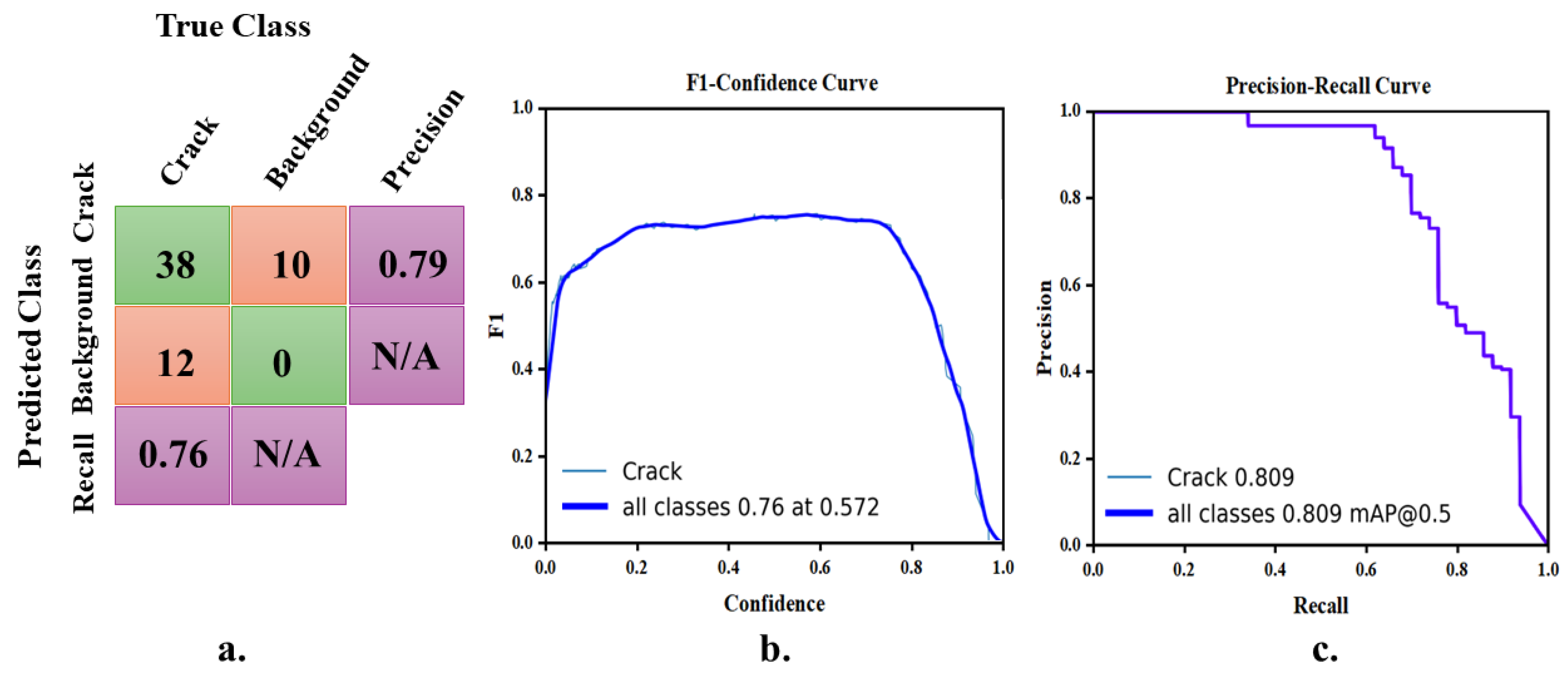
3.3. Quantitative Analysis of Model Performance: Errors and Metrics

To gain a comprehensive understanding of the model’s performance, a multi-metric analysis is essential. The confusion matrix, F1-Confidence curve, and precision–recall (PR) curve offer interconnected insights into the model’s ability to detect cracks.

The confusion matrix in Figure 6a provides valuable insights into the model’s performance and areas for improvement. It demonstrates the model’s strong ability to detect cracks, with a high true positive rate (TPR) of 76%, accurately identifying 38 out of 50 cracks present in the dataset. This high TPR is significant as it showcases the model’s efficacy in recognizing genuine defects, a critical aspect in ensuring the integrity and reliability of 2D materials like hBN.

However, the matrix also reveals the model’s tendency to misidentify 10 background areas (i.e., Si/SiO₂) as cracks, leading to a higher false positive rate (FPR) and lower precision. While this sensitivity (model’s ability to correctly identify actual cracks) ensures that the model errs on the side of caution, it highlights an area for improvement in distinguishing between true cracks and similar anomalies. Enhancing the model’s ability to differentiate between genuine cracks and background irregularities is crucial for reducing unnecessary reviews and interventions in a manufacturing context, ultimately improving both efficiency and cost-effectiveness.

Additionally, the matrix reveals 12 instances where cracks were present but went undetected by the model (false negatives), indicating the need for enhanced sensitivity to ensure fewer cracks are missed, which is critical for quality control in the production of hBN. Given the configuration of the matrix, there is no direct calculation of true negatives (TNs), as the focus is primarily on the detection of cracks, and the background (non-crack areas) is not treated as a separate class. This setup emphasizes the model’s application in scenarios where the primary concern is the reliable detection of cracks rather than the identification of non-crack areas.

The F1–confidence curve (Figure 6b) underscores the inherent trade-off between precision and recall. The model achieves its best balance between these metrics, with an F1 score of 0.76, at a confidence threshold of approximately 0.572. This threshold offers insights into optimizing the model’s crack detection without excessive false alarms.

Figure 6c demonstrates the precision–recall (PR) curve, which provides a more comprehensive view of the trade-off between precision and recall across different classification thresholds. The curve for the “Crack” class starts at a precision of around 0.809, aligning with the maximum F1 score observed in the F1–confidence curve. As the recall increases, the precision decreases, indicating that the model makes more false positive predictions when attempting to capture more true positive instances. The maximum average precision (mAP) across all classes is 0.809 at a recall of 0.5, suggesting that the model performs reasonably well in balancing precision and recall for the “Crack” class. These metrics collectively highlight the model’s strengths and a recurring theme: the trade-off between precision and recall. This analysis sets the stage for investigating how this trade-off evolves during model training.

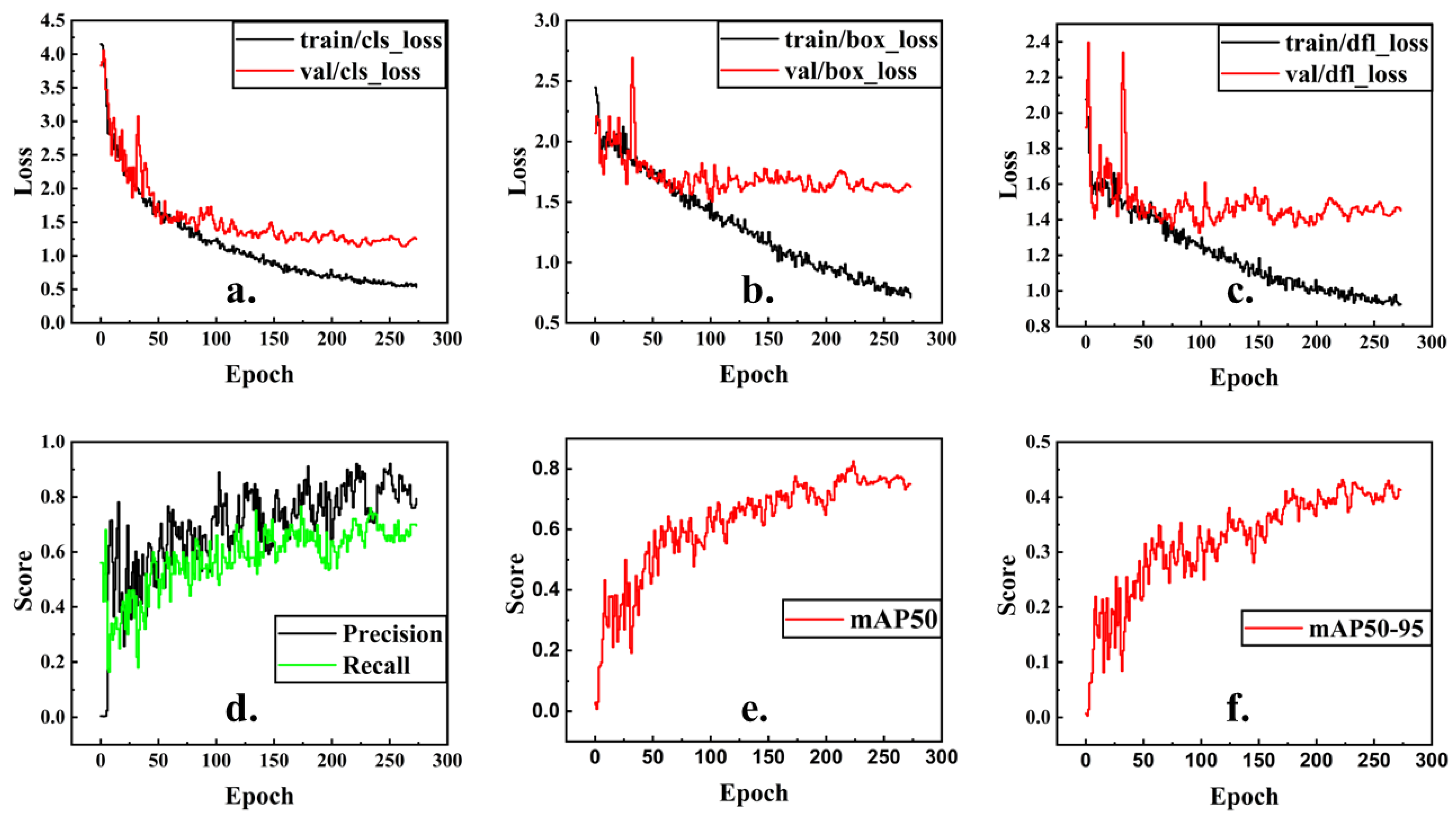
3.4. Understanding Model Training Dynamics: Loss Curve Analysis

Figure 7 offers insights into how the previously discussed precision–recall trade-off evolved during the model’s training process.

Analysis of Figure 7a–c reveals promising trends. The steady decline in training and validation losses across classification loss demonstrates the model’s progressive learning in detecting correct cracks. The validation loss on box loss and distribution focal loss (dfl) saturates after certain epochs. This loss saturation suggests that the model’s bounding box prediction on the data has slight deviation with the actual bounding box. Given our limited dataset (92 images), the model might not encounter enough examples to generalize effectively across broader real-world data variations.

Despite the promising learning trends in classification loss, the plateau in validation loss on box and dfl, resulting in differences between training and validation loss, suggests limited generalizability due to the small dataset and potential data variations not fully represented in the training set.

The precision–recall curves (Figure 7d), with consistently high values and minimal fluctuations, reinforce a favorable balance of precision and recall throughout training. Furthermore, rising mAP50 and mAP50-95 scores (Figure 7e,f) indicate improving crack-detection accuracy, particularly at an IoU threshold of 0.5. While performance at stricter IoU thresholds warrants further investigation, these results collectively show the model’s progressive learning and success in crack detection.

The results highlight the model’s potential for automated crack-detection applications. Its ability to successfully detect diverse cracks, coupled with insights into the precision–recall balance, offers a strong foundation for optimization. Addressing the identified limitations would further bolster the model’s reliability in practical crack inspection scenarios.

4. Discussion

The results presented demonstrate the YOLOv8n model’s potential for crack detection in CVD-grown hBN. Its ability to identify cracks of varying sizes and complexities aligns with the urgent need for streamlined, automated characterization methods in the field of 2D materials. The model’s performance, particularly in detecting diverse crack types, underscores the capabilities of machine learning techniques to address the limitations of traditional optical characterization approaches.

However, the observed trade-off between precision and recall warrants further consideration. This trade-off is consistent with findings in other object detection tasks, highlighting the inherent challenge of balancing the identification of true positives with the minimization of false alarms. The tendency towards false positives, particularly in identifying fine or low-contrast cracks, highlights the core challenge of this work: discriminating between cracks and complex MLhBN regions. This underscores the inherent difficulty of hBN characterization on standard substrates and emphasizes the need for even more precise detection techniques.

An analysis of the model’s learning dynamics offers insights for optimization strategies. The steady decline in classification losses throughout training suggests the model’s progressive knowledge acquisition without significant overfitting. Understanding how the precision–recall balance was learned could inform the use of techniques like class weighting or threshold adjustment to address the observed limitations.

The findings of this study have several implications for research on 2D materials. The demonstrated potential for automated crack detection facilitates the large-scale characterization of CVD-grown hBN. This has direct consequences for quality control and for ensuring material suitability in advanced device applications. Furthermore, the successful application of machine learning underscores its versatility in analyzing complex 2D materials datasets. This lays the groundwork for extending ML-based approaches to address other characterization challenges in the field.

Evaluating the quality of 2D-hBN films based on the detected cracks involves quantifying both the number and size of cracks. While a higher crack density generally suggests a higher degree of defects, the impact on material properties depends on specific application requirements. Even a single large crack can significantly compromise performance in certain applications. Incorporating factors like crack morphology and distribution into the quality assessment process would provide a more comprehensive understanding of the material’s potential performance characteristics. Future work should focus on refining these quantitative quality evaluation methods based on the detected cracks, enabling a more robust and standardized assessment of 2D-hBN films for various applications.

Despite the effectiveness of the YOLOv8n-det model for crack detection, the limitations of using rectangular bounding boxes should be considered. The model may face challenges in distinguishing between closely spaced cracks, as multiple cracks could be identified as a single entity within a bounding box. To address these limitations, future work should explore advanced object detection architectures, such as instance segmentation models (e.g., Mask R-CNN), which provide pixel-level segmentation of cracks instead of rectangular bounding boxes. Additionally, post-processing techniques to refine the detected bounding boxes, such as morphological operations or edge detection algorithms, could be developed to extract the actual crack contours and improve the accuracy of crack area estimation. Semantic segmentation models, which directly classify each pixel as belonging to a crack or background, could also be investigated to handle complex crack patterns and accurately distinguish between nearby cracks. Incorporating a diverse range of crack orientations, shapes, and proximity in the training data would further enhance the model’s ability to handle these challenging scenarios.

Although this study focuses specifically on crack detection due to their critical impact on material properties and device performance, future work should expand the scope to include the detection and characterization of multiple defect types, including residue and wrinkles, as well as address the challenge of distinguishing cracks from complex MLhBN regions. Developing machine learning models capable of identifying and classifying various defects would provide a more holistic understanding of the material’s quality and enable the targeted optimization of the synthesis and transfer processes, accelerating the efficient characterization of 2D-hBN and facilitating its widespread adoption in diverse applications.

While initial development required a labeled dataset and manual annotation, the trained model can now be applied to unlabeled datasets without further human intervention, making it well suited for large-scale analysis. The model’s performance is expected to improve with exposure to larger and more diverse datasets, enhancing robustness and generalizability. Although initially trained on hBN, the model’s approach is highly transferable to other 2D materials. The common practice of characterizing 2D materials on Si/SiO₂ substrates aligns well with the model’s design, which focuses on identifying cracks or discontinuities in a visually distinct layer on a substrate. While the model excels at detecting cracks in optical images, its direct application to studying the underlying mechanisms of crack propagation may be limited, as crack propagation involves complex factors that are not directly evident in simple optical images. However, the model’s ability to identify cracks quickly and accurately could aid in collecting large datasets for further analysis, facilitating the investigation of fundamental principles governing crack formation and propagation in 2D materials.

Several promising avenues exist for future work. Firstly, expanding the dataset with a wider range of crack patterns and substrate contrasts would enhance the model’s robustness in distinguishing fine cracks. Secondly, exploring data augmentation techniques tailored to MLhBN regions could further improve the model’s discriminatory capabilities. Additionally, investigating ensemble methods that combine the strengths of multiple models offers the potential for greater generalizability and accuracy. Finally, the insights gained from this study pave the way for applying the proposed machine learning approach to crack detection in other 2D materials and even complex heterostructures, further accelerating the characterization and development of these advanced materials.

5. Conclusions

This study demonstrates the significant potential of a YOLOv8n-based approach to reliable crack detection in CVD-grown hBN. The model’s success in identifying cracks of varying complexities offers a valuable tool for quality control in hBN production, ensuring its suitability for cutting-edge devices. The observed precision–recall trade-off presents an opportunity for further refinement, with data augmentation and class weighting techniques holding promise for enhancing accuracy. This work advances the practical application of machine learning in 2D materials characterization, streamlining processes and facilitating the widespread adoption of hBN in advanced technologies. By addressing these challenges, machine learning-based characterization has the potential to revolutionize 2D materials development, accelerating the discovery and optimization of novel materials for cutting-edge applications.

References

1. Gupta, A.; Sakthivel, T.; Seal, S. Recent development in 2D materials beyond graphene. Prog. Mater. Sci. 2015, 73, 44–126. [Google Scholar] [CrossRef]
2. Song, L.; Ci, L.; Lu, H.; Sorokin, P.B.; Jin, C.; Ni, J.; Kvashnin, A.G.; Kvashnin, D.G.; Lou, J.; Yakobson, B.I.; et al. Large scale growth and characterization of atomic hexagonal boron nitride layers. Nano Lett. 2010, 10, 3209–3215. [Google Scholar] [CrossRef]
3. Kim, K.K.; Hsu, A.; Jia, X.; Kim, S.M.; Shi, Y.; Dresselhaus, M.; Palacios, T.; Kong, J. Synthesis and characterization of hexagonal boron nitride film as a dielectric layer for graphene devices. ACS Nano 2012, 6, 8583–8590. [Google Scholar] [CrossRef]
4. Roy, S.; Zhang, X.; Puthirath, A.B.; Meiyazhagan, A.; Bhattacharyya, S.; Rahman, M.M.; Babu, G.; Susarla, S.; Saju, S.K.; Tran, M.K.; et al. Structure, Properties and Applications of Two-Dimensional Hexagonal Boron Nitride. Adv. Mater. 2021, 33, 2101589. [Google Scholar] [CrossRef]
5. Zhang, K.; Feng, Y.; Wang, F.; Yang, Z.; Wang, J. Two dimensional hexagonal boron nitride (2D-hBN): Synthesis, properties and applications. J. Mater. Chem. C 2017, 5, 11992–12022. [Google Scholar] [CrossRef]
6. Maity, A.; Grenadier, S.J.; Li, J.; Lin, J.Y.; Jiang, H.X. Hexagonal boron nitride: Epitaxial growth and device applications. Prog. Quantum Electron. 2021, 76, 100302. [Google Scholar] [CrossRef]
7. Ogawa, S.; Fukushima, S.; Shimatani, M. Hexagonal Boron Nitride for Photonic Device Applications: A Review. Materials 2023, 16, 2005. [Google Scholar] [CrossRef]
8. Li, M.; Huang, G.; Chen, X.; Yin, J.; Zhang, P.; Yao, Y.; Shen, J.; Wu, Y.; Huang, J. Perspectives on environmental applications of hexagonal boron nitride nanomaterials. Nano Today 2022, 44, 101486. [Google Scholar] [CrossRef]
9. Zhang, J.; Tan, B.; Zhang, X.; Gao, F.; Hu, Y.; Wang, L.; Duan, X.; Yang, Z.; Hu, P.A. Atomically Thin Hexagonal Boron Nitride and Its Heterostructures. Adv. Mater. 2021, 33, 2000769. [Google Scholar] [CrossRef] [PubMed]
10. Xi, Y.; Zhuang, J.; Hao, W.; Du, Y. Recent Progress on Two-Dimensional Heterostructures for Catalytic, Optoelectronic, and Energy Applications. ChemElectroChem 2019, 6, 2841–2851. [Google Scholar] [CrossRef]
11. Li, Q.; Liu, M.; Zhang, Y.; Liu, Z. Hexagonal Boron Nitride–Graphene Heterostructures: Synthesis and Interfacial Properties. Small 2016, 12, 32–50. [Google Scholar] [CrossRef]
12. Wang, J.; Ma, F.; Sun, M. Graphene, hexagonal boron nitride, and their heterostructures: Properties and applications. RSC Adv. 2017, 7, 16801–16822. [Google Scholar] [CrossRef]
13. Novoselov, K.S.; Mishchenko, A.; Carvalho, A.; Neto, A.H.C. 2D materials and van der Waals heterostructures. Science 2016, 353, 6298. [Google Scholar] [CrossRef]
14. Butler, S.Z.; Hollen, S.M.; Cao, L.; Cui, Y.; Gupta, J.A.; Gutiérrez, H.R.; Heinz, T.F.; Hong, S.S.; Huang, J.; Ismach, A.F.; et al. Progress, challenges, and opportunities in two-dimensional materials beyond graphene. ACS Nano 2013, 7, 2898–2926. [Google Scholar] [CrossRef]
15. Li, X.; Cai, W.; An, J.; Kim, S.; Nah, J.; Yang, D.; Piner, R.; Velamakanni, A.; Jung, I.; Tutuc, E.; et al. Large-area synthesis of high-quality and uniform graphene films on copper foils. Science 2009, 324, 1312–1314. [Google Scholar] [CrossRef]
16. Kim, S.M.; Hsu, A.; Park, M.H.; Chae, S.H.; Yun, S.J.; Lee, J.S.; Cho, D.H.; Fang, W.; Lee, C.; Palacios, T.; et al. Synthesis of large-area multilayer hexagonal boron nitride for high material performance. Nat. Commun. 2015, 6, 8662. [Google Scholar] [CrossRef]
17. Kim, K.K.; Hsu, A.; Jia, X.; Kim, S.M.; Shi, Y.; Hofmann, M.; Nezich, D.; Rodriguez-Nieva, J.F.; Dresselhaus, M.; Palacios, T.; et al. Synthesis of monolayer hexagonal boron nitride on Cu foil using chemical vapor deposition. Nano Lett. 2012, 12, 161–166. [Google Scholar] [CrossRef]
18. Shi, Y.; Hamsen, C.; Jia, X.; Kim, K.K.; Reina, A.; Hofmann, M.; Hsu, A.L.; Zhang, K.; Li, H.; Juang, Z.Y.; et al. Synthesis of few-layer hexagonal boron nitride thin film by chemical vapor deposition. Nano Lett. 2010, 10, 4134–4139. [Google Scholar] [CrossRef]
19. Park, J.H.; Park, J.C.; Yun, S.J.; Kim, H.; Luong, D.H.; Kim, S.M.; Choi, S.H.; Yang, W.; Kong, J.; Kim, K.K.; et al. Large-area monolayer hexagonal boron nitride on Pt foil. ACS Nano 2014, 8, 8520–8528. [Google Scholar] [CrossRef]
20. Chen, C.C.; Li, Z.; Shi, L.; Cronin, S.B. Thermoelectric transport across graphene/hexagonal boron nitride/graphene heterostructures. Nano Res. 2015, 8, 666–672. [Google Scholar] [CrossRef]
21. Chen, Y.; Gong, X.L.; Gai, J.G.; Chen, Y.; Gong, X.L.; Gai, J.G. Progress and Challenges in Transfer of Large-Area Graphene Films. Adv. Sci. 2016, 3, 1500343. [Google Scholar] [CrossRef]
22. Yang, Y.; Song, Z.; Lu, G.; Zhang, Q.; Zhang, B.; Ni, B.; Wang, C.; Li, X.; Gu, L.; Xie, X.; et al. Intrinsic toughening and stable crack propagation in hexagonal boron nitride. Nature 2021, 594, 57–61. [Google Scholar] [CrossRef]
23. Chilkoor, G.; Karanam, S.P.; Star, S.; Shrestha, N.; Sani, R.K.; Upadhyayula, V.K.; Ghoshal, D.; Koratkar, N.A.; Meyyappan, M.; Gadhamshetty, V. Hexagonal Boron Nitride: The Thinnest Insulating Barrier to Microbial Corrosion. ACS Nano 2018, 12, 2242–2252. [Google Scholar] [CrossRef]
24. Chilkoor, G.; Jawaharraj, K.; Vemuri, B.; Kutana, A.; Tripathi, M.; Kota, D.; Arif, T.; Filleter, T.; Dalton, A.B.; Yakobson, B.I.; et al. Hexagonal boron nitride for sulfur corrosion inhibition. ACS Nano 2020, 14, 14809–14819. [Google Scholar] [CrossRef]
25. Watson, A.J.; Lu, W.; Guimaraes, M.H.; Stöhr, M. Transfer of large-scale two-dimensional semiconductors: Challenges and developments. 2D Mater. 2021, 8, 032001. [Google Scholar] [CrossRef]
26. Rahman, M.H.U.; Tripathi, M.; Dalton, A.; Subramaniam, M.; Talluri, S.N.; Jasthi, B.K.; Gadhamshetty, V. Machine Learning-Guided Optical and Raman Spectroscopy Characterization of 2D Materials. In Machine Learning in 2D Materials Science; CRC Press: Boca Raton, FL, USA, 2023; pp. 163–177. [Google Scholar] [CrossRef]
27. Lin, Z.; McCreary, A.; Briggs, N.; Subramanian, S.; Zhang, K.; Sun, Y.; Li, X.; Borys, N.J.; Yuan, H.; Fullerton-Shirey, S.K.; et al. 2D materials advances: From large scale synthesis and controlled heterostructures to improved characterization techniques, defects and applications. 2D Mater. 2016, 3, 042001. [Google Scholar] [CrossRef]
28. Khadir, S.; Bon, P.; Vignaud, D.; Galopin, E.; McEvoy, N.; McCloskey, D.; Monneret, S.; Baffou, G. Optical Imaging and Characterization of Graphene and Other 2D Materials Using Quantitative Phase Microscopy. ACS Photon. 2017, 4, 3130–3139. [Google Scholar] [CrossRef]
29. Bachmatiuk, A.; Schäffel, F.; Warner, J.H.; Rümmeli, M.; Allen, C.S. Characterisation Techniques. In Graphene: Fundamentals and Emergent Applications; Elsevier: Amsterdam, The Netherlands, 2012; pp. 229–332. [Google Scholar] [CrossRef]
30. Gorbachev, R.V.; Riaz, I.; Nair, R.R.; Jalil, R.; Britnell, L.; Belle, B.D.; Hill, E.W.; Novoselov, K.S.; Watanabe, K.; Taniguchi, T.; et al. Hunting for Monolayer Boron Nitride: Optical and Raman Signatures. Small 2011, 7, 465–468. [Google Scholar] [CrossRef]
31. Jordan, M.I.; Mitchell, T.M. Machine learning: Trends, perspectives, and prospects. Science 2015, 349, 255–260. [Google Scholar] [CrossRef]
32. Sikder, R.; Zhang, T.; Ye, T. Predicting THM Formation and Revealing Its Contributors in Drinking Water Treatment Using Machine Learning. ACS ES T Water 2024, 4, 899–912. [Google Scholar] [CrossRef]
33. Gurung, B.D.S.; Khanal, A.; Hartman, T.W.; Do, T.; Chataut, S.; Lushbough, C.; Gadhamshetty, V.; Gnimpieba, E.Z. Transformer in Microbial Image Analysis: A Comparative Exploration of TransUNet, UNet, and DoubleUNet for SEM Image Segmentation. In Proceedings of the 2023 IEEE International Conference on Bioinformatics and Biomedicine (BIBM), Istanbul, Turkey, 5–8 December 2023; IEEE: Piscataway, NY, USA, 2023; pp. 4500–4502. [Google Scholar] [CrossRef]
34. Devadig, R.; Gurung, B.D.S.; Gnimpieba, E.; Jasthi, B.; Gadhamshetty, V. Computational methods for biofouling and corrosion-resistant graphene nanocomposites. A transdisciplinary approach. In Proceedings of the 2023 IEEE International Conference on Bioinformatics and Biomedicine (BIBM), Istanbul, Turkey, 5–8 December 2023; IEEE: Piscataway, NY, USA, 2023; pp. 4494–4496. [Google Scholar] [CrossRef]
35. Gurung, B.D.S.; Devadig, R.; Do, T.; Gadhamshetty, V.; Gnimpieba, E.Z. U-net based image segmentation techniques for development of non-biocidal fouling-resistant ultra-thin two-dimensional (2D) coatings. In Proceedings of the 2022 IEEE International Conference on Bioinformatics and Biomedicine (BIBM), Las Vegas, NV, USA, 6–8 December 2022; IEEE: Piscataway, NY, USA, 2022; pp. 3602–3604. [Google Scholar] [CrossRef]
36. Oruganti, R.K.; Biji, A.P.; Lanuyanger, T.; Show, P.L.; Sriariyanun, M.; Upadhyayula, V.K.; Gadhamshetty, V.; Bhattacharyya, D. Artificial intelligence and machine learning tools for high-performance microalgal wastewater treatment and algal biorefinery: A critical review. Sci. Total. Environ. 2023, 876, 162797. [Google Scholar] [CrossRef] [PubMed]
37. Liu, Y.; Zhao, T.; Ju, W.; Shi, S. Materials discovery and design using machine learning. J. Mater. 2017, 3, 159–177. [Google Scholar] [CrossRef]
38. Yin, H.; Sun, Z.; Wang, Z.; Tang, D.; Pang, C.H.; Yu, X.; Barnard, A.S.; Zhao, H.; Yin, Z. The data-intensive scientific revolution occurring where two-dimensional materials meet machine learning. Cell Rep. Phys. Sci. 2021, 2, 100482. [Google Scholar] [CrossRef]
39. Ryu, B.; Wang, L.; Pu, H.; Chan, M.K.; Chen, J. Understanding, discovery, and synthesis of 2D materials enabled by machine learning. Chem. Soc. Rev. 2022, 51, 1899–1925. [Google Scholar] [CrossRef] [PubMed]
40. Masubuchi, S.; Machida, T. Classifying optical microscope images of exfoliated graphene flakes by data-driven machine learning. npj Mater. Appl. 2019, 3, 4. [Google Scholar] [CrossRef]
41. Masubuchi, S.; Watanabe, E.; Seo, Y.; Okazaki, S.; Sasagawa, T.; Watanabe, K.; Taniguchi, T.; Machida, T. Deep-learning-based image segmentation integrated with optical microscopy for automatically searching for two-dimensional materials. npj Mater. Appl. 2020, 4, 3. [Google Scholar] [CrossRef]
42. Han, B.; Lin, Y.; Yang, Y.; Mao, N.; Li, W.; Wang, H.; Yasuda, K.; Wang, X.; Fatemi, V.; Zhou, L.; et al. Deep-Learning-Enabled Fast Optical Identification and Characterization of 2D Materials. Adv. Mater. 2020, 32, 2000953. [Google Scholar] [CrossRef] [PubMed]
43. Yang, J.; Yao, H. Automated identification and characterization of two-dimensional materials via machine learning-based processing of optical microscope images. Extrem. Mech. Lett. 2020, 39, 100771. [Google Scholar] [CrossRef]
44. Vincent, T.; Kawahara, K.; Antonov, V.; Ago, H.; Kazakova, O. Data cluster analysis and machine learning for classification of twisted bilayer graphene. Carbon 2023, 201, 141–149. [Google Scholar] [CrossRef]
45. Lin, X.; Si, Z.; Fu, W.; Yang, J.; Guo, S.; Cao, Y.; Zhang, J.; Wang, X.; Liu, P.; Jiang, K.; et al. Intelligent identification of two-dimensional nanostructures by machine-learning optical microscopy. Nano Res. 2018, 11, 6316–6324. [Google Scholar] [CrossRef]
46. Li, Y.; Kong, Y.; Peng, J.; Yu, C.; Li, Z.; Li, P.; Liu, Y.; Gao, C.F.; Wu, R. Rapid identification of two-dimensional materials via machine learning assisted optic microscopy. J. Mater. 2019, 5, 413–421. [Google Scholar] [CrossRef]
47. Sterbentz, R.M.; Haley, K.L.; Island, J.O. Universal image segmentation for optical identification of 2D materials. Sci. Rep. 2021, 11, 5808. [Google Scholar] [CrossRef]
48. Ramezani, F.; Parvez, S.; Fix, J.P.; Battaglin, A.; Whyte, S.; Borys, N.J.; Whitaker, B.M. Automatic detection of multilayer hexagonal boron nitride in optical images using deep learning-based computer vision. Sci. Rep. 2023, 13, 1595. [Google Scholar] [CrossRef] [PubMed]
49. Rahman, M.H.U.; Bommanapally, V.; Abeyrathna, D.; Ashaduzzman, M.; Tripathi, M.; Zahan, M.; Subramaniam, M.; Gadhamshetty, V. Machine Learning-Assisted Optical Detection of Multilayer Hexagonal Boron Nitride for Enhanced Characterization and Analysis. In Proceedings of the 2023 IEEE International Conference on Bioinformatics and Biomedicine (BIBM), Istanbul, Turkey, 5–8 December 2023; IEEE: Piscataway, NY, USA, 2023; pp. 4506–4508. [Google Scholar] [CrossRef]
50. Patra, T.K.; Zhang, F.; Schulman, D.S.; Chan, H.; Cherukara, M.J.; Terrones, M.; Das, S.; Narayanan, B.; Sankaranarayanan, S.K. Defect dynamics in 2-D MoS2 probed by using machine learning, atomistic simulations, and high-resolution microscopy. ACS Nano 2018, 12, 8006–8016. [Google Scholar] [CrossRef]
51. Guo, Y.; Kalinin, S.V.; Cai, H.; Xiao, K.; Krylyuk, S.; Davydov, A.V.; Guo, Q.; Lupini, A.R. Defect detection in atomic-resolution images via unsupervised learning with translational invariance. npj Comput. Mater. 2021, 7, 180. [Google Scholar] [CrossRef]
52. Lee, C.H.; Khan, A.; Luo, D.; Santos, T.P.; Shi, C.; Janicek, B.E.; Kang, S.; Zhu, W.; Sobh, N.A.; Schleife, A.; et al. Deep learning enabled strain mapping of single-atom defects in two-dimensional transition metal dichalcogenides with sub-picometer precision. Nano Lett. 2020, 20, 3369–3377. [Google Scholar] [CrossRef] [PubMed]
53. Li, X.; Zhu, Y.; Cai, W.; Borysiak, M.; Han, B.; Chen, D.; Piner, R.D.; Colomba, L.; Ruoff, R.S. Transfer of large-area graphene films for high-performance transparent conductive electrodes. Nano Lett. 2009, 9, 4359–4363. [Google Scholar] [CrossRef] [PubMed]
54. Fukamachi, S.; Solís-Fernández, P.; Kawahara, K.; Tanaka, D.; Otake, T.; Lin, Y.C.; Suenaga, K.; Ago, H. Large-area synthesis and transfer of multilayer hexagonal boron nitride for enhanced graphene device arrays. Nat. Electron. 2023, 6, 126–136. [Google Scholar] [CrossRef]
55. Park, H.; Lim, C.; Lee, C.J.; Kang, J.; Kim, J.; Choi, M.; Park, H. Optimized poly(methyl methacrylate)-mediated graphene-transfer process for fabrication of high-quality graphene layer. Nanotechnology 2018, 29, 415303. [Google Scholar] [CrossRef]
56. Liu, Z.; Gong, Y.; Zhou, W.; Ma, L.; Yu, J.; Idrobo, J.C.; Jung, J.; Macdonald, A.H.; Vajtai, R.; Lou, J.; et al. Ultrathin high-temperature oxidation-resistant coatings of hexagonal boron nitride. Nat. Commun. 2013, 4, 2541. [Google Scholar] [CrossRef]
57. Ultralytics. YOLOv5: A State-Of-The-Art Real-Time Object Detection System. 2021. Available online: https://docs.ultralytics.com (accessed on 30 March 2024).
58. Wang, C.Y.; Mark Liao, H.Y.; Wu, Y.H.; Chen, P.Y.; Hsieh, J.W.; Yeh, I.H. CSPNet: A New Backbone that can Enhance Learning Capability of CNN. In Proceedings of the 2020 IEEE/CVF Conference on Computer Vision and Pattern Recognition Workshops (CVPRW), Virtual, 14–19 June 2020; IEEE: Piscataway, NY, USA, 2020. [Google Scholar] [CrossRef]
59. Ju, R.Y.; Cai, W. Fracture detection in pediatric wrist trauma X-ray images using YOLOv8 algorithm. Sci. Rep. 2023, 13, 20077. [Google Scholar] [CrossRef] [PubMed]
60. Lin, T.Y.; Dollar, P.; Girshick, R.; He, K.; Hariharan, B.; Belongie, S. Feature Pyramid Networks for Object Detection. In Proceedings of the IEEE Conference on Computer Vision and Pattern Recognition (CVPR), Honolulu, HI, USA, 21–26 July 2017. [Google Scholar] [CrossRef]
61. Liu, S.; Qi, L.; Qin, H.; Shi, J.; Jia, J. Path Aggregation Network for Instance Segmentation. In Proceedings of the 2018 IEEE/CVF Conference on Computer Vision and Pattern Recognition, Salt Lake City, UT, USA, 18–22 June 2018; pp. 8759–8768. [Google Scholar] [CrossRef]
62. Feng, C.; Zhong, Y.; Gao, Y.; Scott, M.R.; Huang, W. TOOD: Task-aligned One-stage Object Detection. In Proceedings of the 2021 IEEE/CVF International Conference on Computer Vision (ICCV), Montreal, QC, Canada, 10–17 October 2021. [Google Scholar] [CrossRef]
Figure 1. Accelerating hBN characterization: A machine learning workflow for automated crack detection. Our comprehensive workflow integrates material synthesis, image acquisition, meticulous annotation, the fine-tuning of a YOLOv8n deep learning model, and rigorous evaluation to streamline hBN quality control and accelerate its use in advanced devices.
Coatings 14 00726 g001
Figure 2. Architecture of the YOLOv8 model: backbone, neck, and head with component modules. Reprinted with permission from Ref. [59]. 2019, Springer Nature.
Coatings 14 00726 g002
Figure 3. Multi-technique characterization of transferred hBN film: (a) The optical image reveals the overall morphology; (b) SEM highlights the edge and substrate topography, and the image was obtained with the Everhart–Thornley Detector (ETD) at 5 kV accelerating voltage; (c) AFM height image; (d) line scans quantify thickness variations; (e) Raman (crack regions); (f) Raman (hBN film).
Coatings 14 00726 g003
Figure 4. Crack detection with proposed algorithm. (a) Raw image. (b) Model-generated crack detections with bounding boxes and confidence scores. (c,d) Close-ups demonstrate the accurate identification of varying crack types. Scale bars, (a,b) 200 μ m.
Coatings 14 00726 g004
Figure 5. Model-generated crack detections and analysis. (af) Model output with bounding boxes and confidence scores. Analysis highlights strengths and weaknesses. Scale bars, (af) 200 μ m.
Coatings 14 00726 g005
Figure 6. Multi-metric analysis of crack-detection model performance: (a) Raw confusion matrix reveals true positives, false positives, and potential class imbalance, where N/A values reflect that only the crack class is used for testing and the background is irrelevant for evaluation; (b) F1-Confidence curve pinpoints optimal confidence threshold; (c) precision–recall curve maps precision decay as recall increases, highlighting the model’s overall performance trade-offs.
Coatings 14 00726 g006
Figure 7. Multi-metric evaluation of the YOLOv8n model’s training progress. (a) Classification, (b) bounding box, and (c) distribution focal loss curves reveal steady improvement; (d) precision–recall curves demonstrate strong performance; (e,f) increasing mAP50 and mAP50-95 scores indicate improving object detection accuracy.
Coatings 14 00726 g007