2.1. RNA Expression Data
In this study, mRNA expression data, miRNA expression data, lncRNA expression data and clinical data were collected from the open-access dataset of The Cancer Genome Atlas (TCGA) database [
13]. The project ID was “TCGA-COAD”.
For mRNA and lncRNA expression data, the experimental strategy we downloaded was “RNA-Seq”, the data type was “Gene Expression Quantification”, and the data category was “transcriptome profiling”. The data from the Ensemble database [
14] annotated the type of all RNAs in the gene expression data, and it was downloaded from TCGA. In this study, we selected “protein-coding gene” and “lncRNA” as mRNA and lncRNA for subsequent analysis.
For miRNA, the data type we downloaded was “Isoform Expression Quantification”, the workflow type was “BCGSC miRNA Profiling”, and the data category was “Transcriptome Profiling”.
The clinical data of colon cancer were also obtained from TCGA. The original clinical data contained a variety of clinical information items of the samples, and only the information about sample ID and cancer stage was selected. The sample ID was used to map the RNA expression data of the particular sample, and the information of the cancer stage was used to distinguish whether the samples were cancerous or paracancerous tissue; the latter will be used as normal samples.
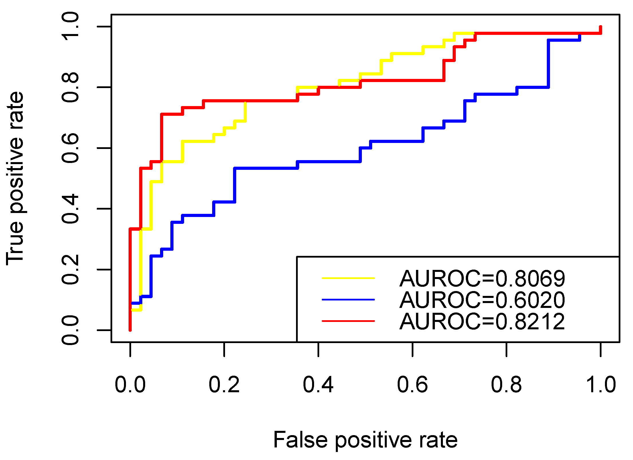
2.7. RW-DIR
Similarly to traditional random walk, RW-DIR required a transition matrix [
26] for the subsequent walk in the network, but the transition matrix in this study was designed based on heterogeneous networks. A diagram of the calculation method is shown in
Figure 3. In the figure,
s represents the number of mRNAs,
m represents the number of miRNAs,
n represents the number of lncRNAs, and
h represents the number of all RNAs. Obviously,
h equals to the sum of
s,
m, and
n. Three parameters,
,
and
, are used to adjust the transition probability of different types of RNAs. The
is the transfer parameter between mRNA and miRNA, the
is the transfer parameter between mRNA and lncRNA, and the
is the transfer parameter between miRNA and lncRNA. Specifically, we have the following.
The method to calculate transition matrix W is written as Equation (
4):
where
,
,
,
and
. The selection of parameter
X,
a and
b could be more intuitive according to the
Figure 3. Since H was comprised 9 sub-matrices, the sub-matrices should be calculated separately.
Random walk is a discrete-time Markov process where a walker located at vertex
i at a certain moment will jump to adjacent vertex
j at the next moment with probability
. This jump is independent to the past. Before exhibiting random walk with dynamic incentive restart (RW-DIR), we introduced the random walk with restart (RWR) method [
27] first. The difference between RWR and traditional random walk is that there is a certain probability of returning to the starting point after each step of walking. In RWR, based on the transition matrix
W and the hopping process
=
, where
is a vector that represents the probability of walker at all vertex at time
t, and
will converge, which means RWR will reach a stationary distribution.
Next, we would introduce RW-DIR. The vertices in the studied heterogeneous network have certain prior knowledge about colon cancer; thus, we considered that in the process of walking. Different measures should be taken for vertices with different labels such that the reliable colon cancer-related vertices can be finally obtained. The specific algorithm process is defined in Algorithm 1. In the initial round of the algorithm, we assigned the value of 1 in
to the colon cancer-related RNA with the largest degree, and the rest was 0. In each round of the algorithm, judging which vertices the current round walks to was based on whether there were any changes in
compared with
. Considering that the random walk process could spread the information of labelled RNAs, we used known knowledge for random walk and information dissemination. We inflated the effect of the “related” vertex, which was gradually added to
. It enhanced its global influence in the process of repeatedly restarting. We shrunk the effect of the “irrelevant” vertex, which included adding a penalty value to the “irrelevant” vertex in each iteration to make it smaller; this would reduce their impact of the global process. For the “unlabeled” vertex, we referred to the idea of maximum entropy by calculating the entropy value of each vertex after each iteration, and the inference result of the vertex with the largest entropy value represented the highest uncertainty. The transition probability matrix
W is recalculated according to the entropy value in each round iteration. The larger the entropy value, the larger transition probability matrix value of the vertex. It should be noted that the calculation of entropy needs to be started after walking to the global process; that is, the calculation of the transfer matrix also needs to wait until the process of walking to all vertices. It would help the vertex with the “unlabeled” result in collecting more information for further inferences.
| Algorithm 1 Random Walk with Dynamic Incentive Restart (RW-DIR) |
![Biology 11 01003 i001]() |
The entropy value
of the vertex
can be calculated by Equation (
5), where
represents the possibility that vertex
belonged to label
k. In this study, we set
represent the “related” vertex, and
represent the “irrelevant” vertex. When the
value of vertex
is calculated for the first time (the
tth round walk), where
was the “unlabeled” vertex, we obtain initial
=
, and
= 1−
. For “related” vertex
, we set
= 1 and
= 0. For “irrelevant” vertex
, we set
= 1 and
= 0.
When the random walk process had covered the entire network (in the
tth round walk), transition matrix
W needed to be updated according to the entropy value of E by Equation (
6), where
represented all neighbor vertices of
, including
.
After that, it was necessary to update and calculate the probability that each vertex belonged to each label. As shown in Equation (
7),
represented the probability that label k propagated from vertex
to vertex
, which could be used to further calculate the probability of vertex
with label k, i.e.,
, in Equation (
8).
In summary, at the beginning of the algorithm, we started the RW-DIR algorithm with one known colon cancer-related vertex. In the subsequent iterative process of the walker, compared to the previous round, we classified the type of vertices that had been “walked”. If it was a “related” vertex that has never been reached before, it would be added to P0 and assigned a value of 0.1. If it was an “irrelevant” label, add a penalty value to ; that is, we divide it by its degree. If the walker “walked” to vertices with no label, its entropy value would be calculated, and the transition matrix should be updated by the entropy value. Finally, the algorithm would stop after convergence. The sorting result of the unlabeled vertex will be used as an indicator for screening colon cancer-related RNAs.


