Solute Transport across the Lymphatic Vasculature in a Soft Skin Tissue

Simple Summary

The lymphatic system plays a crucial role in maintaining fluid and solute balance in biological tissue, which makes the subcutaneous injection a common approach for delivering therapeutic agents through the lymphatic pathway. The transport of drug solutes is regulated by the interstitial fluid pressure. In our study, a time-efficient poroelastic model is developed to mimic pressure relaxation and build-up in the soft skin tissue. This method can accurately and time-efficiently capture the evolution of pressure, which is validated against both the analytical solution and numerical solution of the previous poroelastic model. The increasing porosity and permeability due to deformation alleviate the high pressure caused by the injection. Furthermore, an improved solute transport model is developed to better address the microscopic properties of the lymphatic vessel membrane. The effects of a varying Stokes radius of drug solute and vessel network structures are investigated on lymphatic uptake. Our comprehensive computation model provides a time-efficient and reliable research tool for studying solute transport into the lymphatic system, which can be utilized to support decision-making regarding lymphatic disturbed diseases.

Abstract

Convective transport of drug solutes in biological tissues is regulated by the interstitial fluid pressure, which plays a crucial role in drug absorption into the lymphatic system through the subcutaneous (SC) injection. In this paper, an approximate continuum poroelasticity model is developed to simulate the pressure evolution in the soft porous tissue during an SC injection. This poroelastic model mimics the deformation of the tissue by introducing the time variation of the interstitial fluid pressure. The advantage of this method lies in its computational time efficiency and simplicity, and it can accurately model the relaxation of pressure. The interstitial fluid pressure obtained using the proposed model is validated against both the analytical and the numerical solution of the poroelastic tissue model. The decreasing elasticity elongates the relaxation time of pressure, and the sensitivity of pressure relaxation to elasticity decreases with the hydraulic permeability, while the increasing porosity and permeability due to deformation alleviate the high pressure. An improved Kedem–Katchalsky model is developed to study solute transport across the lymphatic vessel network, including convection and diffusion in the multi-layered poroelastic tissue with a hybrid discrete-continuum vessel network embedded inside. At last, the effect of different structures of the lymphatic vessel network, such as fractal trees and Voronoi structure, on the lymphatic uptake is investigated. In this paper, we provide a novel and time-efficient computational model for solute transport across the lymphatic vasculature connecting the microscopic properties of the lymphatic vessel membrane to the macroscopic drug absorption.

1. Introduction

The lymphatic vascular system returns the interstitial fluid to the systemic circulation in the human body, which plays an essential role in homeostasis and immunization in the human body [1,2,3,4]. Changes or defects in the lymphatic vascular function can induce variable human body responses to a wide range of human diseases, such as obesity and Alzheimer’s disease [4]. The lymphatic pathway is a common approach for the delivery of large therapeutic proteins, such as monoclonal antibodies, through subcutaneous (SC) injection [2,3,5,6]. SC injection has many merits, such as lower cost and convenience compared to intravascular (IV) injection [7,8,9]. In a recent administration analysis, subcutaneous injection takes up $76\%$ of all the US FDA-approved administration of therapeutic agents of high concentration [10]. After being injected into the subcutaneous tissue, drug solutes transport into the initial lymphatics, deeper collecting lymphatics and then lymph nodes, and at last, into the systemic circulation [2]. During the transport process, many internal and external factors affect drug absorption after subcutaneous injection, such as the physiological properties of the subcutaneous tissues, injection site, drug and formulation properties, and administration mode [6]. The quantitative investigation on the subcutaneous absorption through physics-based computational modeling bridges the gap between the understanding of the absorption process through SC injection and the development of drug and drug delivery system.

In our previous works [11,12,13], the convective transport of drug solutes is driven by the interstitial fluid pressure (IFP) into the lymphatic system, which plays an important role in drug absorption through SC injection. The mechanical process of the injection and its effect on pressure build-up and relaxation are essential to understand the fluid flow and drug clearance at the injection site [12,14]. The diffusion across the discrete heterogeneous lymphatic vessel network significantly affects the lymphatic uptake [13]. However, the computation cost is expensive for a multi-scale problem with both a heterogeneous explicit vessel network and the constitutive equations included, where the vessels of radius O (10 $\mathsf{\mu }$m) are embedded in a domain of size O (1 cm). A time-efficient and accurate biomechanical model for pressure evolution can be valuable to such a complex computational system to study the transport and absorption of large drug molecules in biological tissues.

The pressure build-up in subcutaneous tissue during the subcutaneous injection has been investigated through experiments in several previous studies [15,16]. The counter pressure in the subcutaneous tissue is estimated based on experimental data, and a model for the pressure evolution is constructed [15]. The experiments of subcutaneous injection show that controlling the injection rate could be used to partially prevent back pressure from increasing to unacceptable ranges, while changing the injection volume alone shows little influence on pressure evolution [17]. The X-ray imaging technique is used to study the effects of injection conditions on the permeation of the drug in tissues [18] in horizontal and vertical directions for different injection speeds. Due to the lack of in situ quantitative experiments on IFP and lymphatic uptake at the injection site, numerical simulations are used to improve our understanding of the effects of the tissue mechanical properties on drug delivery. The effect of the biomechanical responses of the soft tissue on the fluid flow is investigated by coupling Darcy’s law with stress–strain behaviors for the solid skeleton, i.e., the constitutive models. The poroelastic model is widely used to describe the deformation of biological tissues and hydrogels [12,14,19,20]. Our previous studies numerically investigate the contribution of large interstitial pressure to drug absorption during and after the injection [11,12]. A hybrid discrete-continuum vessel network model is developed to describe the diffusion and convection of drug solutes across the vessel wall [13]. Although the poroelastic model can simulate the deformation of the soft subcutaneous tissue, the computation is expensive after coupling with transport equations and instability issues may occur [12]. Including a three-dimensional (3D) heterogeneous vessel network in the simulations can make the computations more expensive. A few methods are used to simplify the computations in the literature. One approach is reducing the dimension of the numerical simulation. The mathematical equations for the interstitial fluid flow and soft tissue strain are solved in two-dimensional models using a finite element method to study the effect of strain relaxation on fluid drainage and solute transport [21,22], while one-dimensional mathematical models are also used to analyze the fluid flow and solute transport [23]. Another approach is simplifying the stress–strain relation to make the computations more efficient. The linear poroelasticity based on small strain theory is often used to simplify the constitutive Equation [24]. In [25], the deformation and strain are obtained by simplifying the poroelastic constitutive equation to simulate the deformation of a hydrogel. In this paper, we develop a new approximate poroelastic model to mimic the relaxation of the pressure in soft tissues.

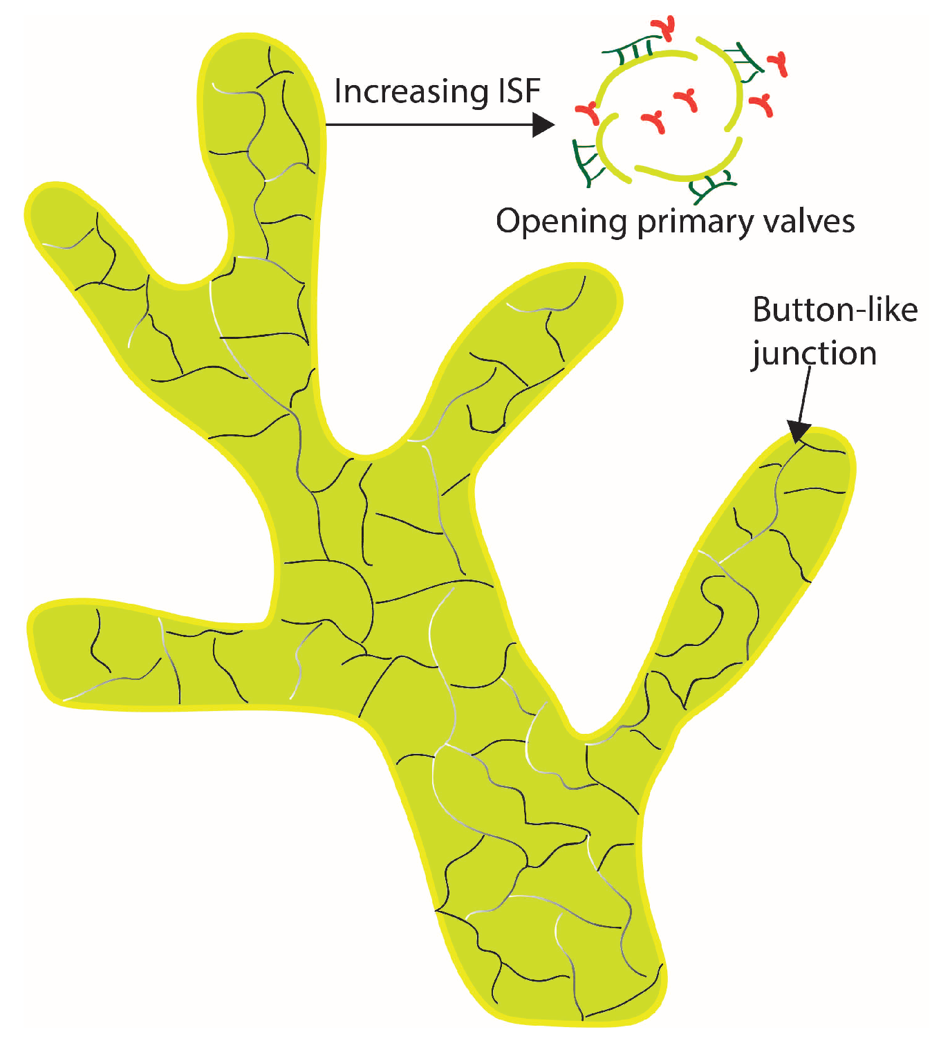
As one of the two vascular circulatory systems in the human body, the lymphatic vessel network consists of initial lymphatics with only one single layer of lymphatic endothelial cells (LECs), unlike blood vessels which have a complete basement membrane [2,3,4]. For lymphatic vessels, LECs are loosely connected and have a primary valve structure to ensure the one-directional fluid flows from the interstitial space into the lymphatics. In our previous work [13], three different transport conditions are used to investigate solute transport across the lymphatic vessel membrane, including the Kedem-Katchalsky model. In [26,27], an integral form of the modified Kedem–Katchalsky formulation is used to study dermal clearance through the blood and lymphatic vessels. To further address the special physiological structure of the lymphatic vessel membrane, in this paper, we develop an improved Kedem–Katchalsky model for solute transport across the explicit lymphatic vessel wall. The morphology of the initial lymphatic vessel network varies over the location and species [3]. In human skin tissue, blind-ended and interconnected structures (reticular plexus) are observed for initial lymphatic vessels [28,29,30,31]. However, there is no quantitative investigation on the effect of various structures of the lymphatic vessel network on solute transport and absorption through the lymphatic vessel network.

In this paper, an approximate continuum poroelastic model is developed to simulate the pressure evolution in the soft subcutaneous tissue. The pressure evolution of the proposed model is quantitatively validated against the analytical solution and the numerical solution of the poroelasticity model. The effect of elasticity, variable porosity and permeability on pressure build-up is numerically investigated. The convective and diffusive transport of drug solute into the lymphatic vessels is investigated through an improved Kedem–Katchalsky model by implementing the hybrid vessel network in the continuum poroelastic model. At last, heterogeneous vessel networks with various structures are used to investigate the effect of the morphology of the lymphatics on solute transport into the lymphatic system in the multi-layer soft skin tissue.

2. Methodology

To simulate the microcirculation in the subcutaneous tissue, the physics-based computational model established in this study is combined with physiological models, i.e., transvascular transport models. A continuum approximate poroelasticity model is developed to simulate the interstitial fluid flow in soft subcutaneous tissue. In this section, the governing equations for fluid flow and drug solute transport in the interstitial space and across the vessel network are summarized.

2.1. Poroelastic Tissue Model

An approximate poroelasticity model is developed to include the elasticity and compressibility of the skin tissue. This method is both simple and efficient, making it easy to implement. The computational cost is reduced since the constitutive equation to obtain the displacement of a solid skeleton is not solved. At the same time, it can well capture the relaxation of pressure as accurately as the full poroelasticity model [14]. Here, we show the derivation of the approximate poroelasticity model from the Biot poroelasticity theory [32,33,34]. The total stress $\tau$ of the poroelastic medium is the sum of the effective stress of the solid skeleton (responsible for the deformation of the solid part of the tissue) and the local fluid pressure as follows:

$$\tau =\sigma -\alpha p\mathit{I},$$

(1)

where $\sigma$ represents the components of effective stress applied to the solid part of the medium, p represents the pore pressure applied to the fluid, and $\alpha$ is the Biot’s coefficient. For an incompressible fluid, $\alpha =1$. Here, $\mathit{I}$ is the identity matrix. Using the force balance, $\nabla ·\tau =0$, we have:

$$\nabla ·\mathsf{œ}-\alpha \nabla p=0.$$

(2)

Based on Biot’s poroelasticity theory [32,34], one form of governing equation for the fluid flow in the poroelastic medium is [14,34,35]:

$$\alpha \frac{\partial {\epsilon }_v}{\partial t}+\frac{1}{M}\frac{\partial p}{\partial t}=\nabla ·\left(\frac{\kappa }{\mathsf{\mu }}\nabla p\right),$$

(3)

where $\kappa$ is the permeability of the porous medium $\mathsf{\mu }$ is the viscosity of the fluid, ${\epsilon }_v$ is the volumetric strain and M is the bulk modulus of the fluid-solid mixture.

For the approximate poroelasticity model, we assume that solid displacement is small, the Darcy velocity of the interstitial fluid is small, and the non-zero component of the solid displacement $\mathbf{ı}$ is mainly in the normal direction. Based on our homogeneous and small strain assumption (linear elasticity), we have $\sigma =E\epsilon$ in one dimension, i.e., Hooke’s law for the elastic response, where E is Young’s modulus of the elasticity. For a 3-D simulation, the volumetric dilation is ${\epsilon }_v=\sum {\epsilon }_i=\partial {\mathbf{ı}}_i/\partial x_i$ [36], where $\mathbf{ı}$ is the displacement of the solid. We have the mean stress $\overline{\mathsf{œ}}={\sigma }_{ii}/3=E_v{\epsilon }_{ii}=E_v{\epsilon }_v$, where $E_v=E/3(1-2\nu )$. After applying the stress balance ($E_v{\epsilon }_v=\alpha p$), we obtain the approximation for the time derivative of the volumetric strain ${\epsilon }_v$ as below:

$$\frac{\partial {\epsilon }_v}{\partial t}=\frac{\partial \nabla ·\mathbf{ı}}{\partial t}=\frac{\alpha }{E_v}\frac{\partial p}{\partial t}.$$

(4)

Finally, the pressure equation for the poroelastic tissue becomes:

$$(\frac{\alpha }{E_v}+\frac{1}{M})\frac{\partial p}{\partial t}-\nabla ·\left(\frac{\kappa }{\mathsf{\mu }}\nabla p\right)=0.$$

(5)

The mass balance in the interstitial space with solid displacement $\mathbf{ı}$ reads as [21],

$$\nabla ·\dot{\mathbf{ı}}-\nabla ·\left(\frac{\kappa }{\mathsf{\mu }}\nabla p\right)=0,$$

(6)

where $\dot{\mathbf{ı}}$ is the time derivative of deformation $\dot{\mathbf{ı}}=\partial \mathbf{ı}/\partial t$, i.e., the velocity of the solid skeleton ${\mathbf{u}}_{\mathbf{s}}$. We define $1/D_e=\alpha /E_v+1/M$, where $D_e$ indicates the general softness of the tissue. After combining Equations (5) and (6), we have the governing equation for the approximate deformation:

$$\nabla ·\nabla \zeta -\frac{1}{D_e}\nabla p=0.$$

(7)

The details of the injection model and the qualification of the proposed continuum poroelasticity model can be found in Appendix A.1 and Appendix A.2, respectively. When utilizing 96-processors parallel computation, it takes approximately one day to complete a simulation using the approximate poroelasticity model, which models the transport and pressure evolution in a poroelastic tissue up to 70 s after the start of the injection. The efficiency of our proposed model is comparable to Darcy’s law model for the porous medium [11]. However, it takes three days to finish the same simulation solving the constitutive equation of poroelasticity [12]. The approximate poroelasticity model improves the computational efficiency by three times compared to the full poroelasticity model.

2.2. Transport Equations

A comprehensive model for the extravascular transport of fluid and drug solutes and the transvascular exchange in the tissue is described for both the continuum medium over the length scale of O (1 cm) and the discrete vessels over the length of O (100 $\mathsf{\mu }$m) in this Section [11,13].

2.2.1. Fluid Flow in the Interstitial Space

First, Darcy’s law is used to describe the fluid flow in the porous media:

$${\mathbf{u}}_{\mathbf{D}}=-\frac{k}{\mathsf{\mu }}\nabla p,$$

(8)

where ${\mathbf{u}}_{\mathbf{D}}$ is the average velocity of interstitial fluid flow in the porous medium, and ${\mathbf{u}}_{\mathbf{D}}={\mathbf{u}}_{\mathbf{f}}-{\mathbf{u}}_{\mathbf{s}}$, where ${\mathbf{u}}_{\mathbf{f}}$ is the fluid velocity in the pore. On the right-hand side (RHS) of Equation (8), p is the interstitial pressure and $\mathsf{\mu }$ is the dynamic viscosity of the interstitial fluid.

With the flux gain from blood vessels and drainage from lymphatics included, the continuity equation considering the poroelasticity gives [1,37,38,39,40]:

$$\nabla ·{\mathbf{u}}_{\mathbf{D}}+\nabla ·\dot{\mathbf{ı}}=q_r+J_v-J_l,$$

(9)

where $J_v$ and $J_l$ are the net fluid flux gain from blood vessels and net fluid flux loss to lymphatic vessels per tissue unit volume, respectively, and $q_r$ is the source term, representing the injection. For the fluid flow in the proposed approximate poroelastic equation, it satisfies Equations (5) and (6), i.e., $\nabla ·\dot{\mathbf{ı}}=1/D_e\partial p/\partial t$. The fluid conservation equation for a poroelastic medium without any source term could be written as [5,41]. After substituting Equation (8) and the expression for $\nabla ·\dot{\mathbf{ı}}$ into Equation (9), we have the governing equation for pressure:

$$\frac{1}{D_e}\frac{dp}{dt}-\nabla ·\left(\frac{k}{\mathsf{\mu }}\nabla p\right)=\left(q_r+J_v-J_l\right).$$

(10)

The net fluid fluxes through the blood and lymphatic vessels are determined by Starling’s law, which read [37,38,39,40]:

$$\begin{array}{cc}\hfill J_v& =L_{pv}\frac{S}{V}(p_v-p_i-\sigma ({\pi }_v-{\pi }_i)),\hfill \end{array}$$

(11)

$$\begin{array}{cc}\hfill J_l& =L_{pl}\frac{S}{V}(p_i-p_l),\hfill \end{array}$$

(12)

where $L_{pb}$ and $L_{pl}$ are the hydraulic conductivity of blood and lymphatic vessels, respectively. Additionally, $S/V$ denotes the surface area of vessels to the unit volume of tissue. Pressures in blood, lymphatics, and the interstitial space are $p_v$, $p_l$, and $p_i$, respectively. In Equation (11), $\sigma$ is the osmotic reflection coefficient of blood capillary for the solute, where ${\pi }_v$ and ${\pi }_i$ are the osmotic pressures of the plasma in the blood vessel and the interstitial space, respectively.

2.2.2. Solute Transport in the Interstitial Space

A general solute transport equation at the macroscopic scale is used for the continuum model [11,13,37,38,42]:

$$\frac{\partial \epsilon C}{\partial t}+\nabla ·\left({\mathit{u}}_{\mathit{D}}C\right)=\nabla ·(D\epsilon \nabla C_i)+q_r+{\varphi }_b-{\varphi }_e-{\varphi }_l,$$

(13)

where C is the dimensionless drug concentration in the interstitium, normalized by the initial concentration $C_0$. The effective molecular diffusion coefficient in the interstitial space is denoted as D. On the right-hand side, ${\varphi }_e$ denotes the elimination of the drug per tissue unit volume due to binding to the ECM and cells, cell uptake, or chemical reaction, ${\varphi }_b$ denotes drug perfusion from blood vessels, and ${\varphi }_l$ denotes drug drainage to lymphatic vessels. Drug absorption through lymphatic vessels is given by ${\varphi }_l=J_l{C}_i$ [38,42,43]. In Equation (13), ${\varphi }_b$ is set to be zero, considering that large molecules cannot directly transport into blood vessels. The elimination term (${\varphi }_e$) is set to be zero except in the section studying the role of binding and metabolism to focus on the transport and absorption of free drug molecules.

2.2.3. Transvascular Fluid Flow and Solute Transport

The well-known model for solute transport across the membrane, the Kedem–Katchalsky (K-K) formulation, is used for solute transport across the blood vessels. The fluid and solute fluxes are expressed as:

$$\begin{array}{cc}\hfill J_B{|}_{\partial {\Omega }_B}& =L_{pb}\epsilon (p_b-p_i-{\sigma }_b({\pi }_b-{\pi }_i)),\hfill \end{array}$$

(14)

$$\begin{array}{cc}\hfill j_{bs}{|}_{\partial {\Omega }_B}& =J_B{|}_{\partial {\Omega }_B}(1-{\sigma }_b)(C+C_b)/2+P_b^{\alpha }\Delta C,\hfill \end{array}$$

(15)

where $J_B$ denotes the fluid flux and $j_{bs}$ denotes the solute flux per unit area across the blood capillary wall consisting of the convective and diffusive transport of solute across the vessel wall (i.e., membrane). The convective transport of solute is determined by the convective fluid flow $J_B{|}_{\partial {\Omega }_B}$, while the diffusive transport of solute is determined by the solute permeability $P_b^{\alpha }$. The average concentration across the membrane is calculated by $(C+C_b)/2$, where $C_b$ is the concentration of drug solution inside the blood vessels and C is the concentration in the interstitial space. Here, all concentrations are normalized by the initial concentration of the injected drug solution $C_0$. The diffusive transport is determined by the difference between the concentration in the interstitial space and the blood vessels $\Delta C$, which is calculated by $C-C_b$. The reflection coefficient $\sigma$ and the solute permeability $P_b$ are used to take into account the permeability of the blood vessel membrane for various solutes. Considering that large molecules (such as monoclonal antibodies with molecular weight over 150 kPa) cannot transport through the blood vessels, we have $\sigma =1$ and $P_b=0$ to represent a semipermeable membrane [13].

The lymphatic vessel consists of one single layer of endothelial cells lacking the basement membrane and thus, an improved Kedem–Katchalsky (iK-K) model is developed to describe the transport of macromolecules across the lymphatic vessel wall. The fluid flux $J_L$ and solute flux $j_{ls}$ across the lymphatic vessel wall are:

$$\begin{array}{cc}\hfill J_L{|}_{\partial {\Omega }_L}& ={\delta }_{valve}{L}_{pl}\epsilon (p_i-p_l),\hfill \end{array}$$

(16)

$$\begin{array}{cc}\hfill j_{ls}{|}_{\partial {\Omega }_L}& =J_L{|}_{\partial {\Omega }_L}(1-{\sigma }_l)(C_l+C)/2+P_{valve}(C-C_l).\hfill \end{array}$$

(17)

where ${\delta }_{valve}$ is used to represent the primary valve structure of the initial lymphatics, where slits are opened when the interstitial pressure (ISF) $p_i$ is larger than the pressure inside the lymphatics $p_l$. The primary valves openings allow for the transport of large molecules into initial lymphatics, as shown in Figure 1. Solute permeability through the valve $P_{valve}$ is related to the partition coefficient of the solute $\mathrm{\Phi }$, which is a function of the Stokes radius of the solute, primary valve opening area fraction ${\delta }_f$, and diffusion across the opening slit $D_{valve}$.

$$\begin{array}{cc}\hfill P_{valve}& ={\delta }_f{D}_{valve}\mathrm{\Phi }\left(r_s\right)/d_l,\hfill \end{array}$$

(18)

$$\begin{array}{cc}\hfill \mathrm{\Phi }\left(r_s\right)& ={\delta }_{valve}^{\prime }(1-\frac{r_s}{w/2}).\hfill \end{array}$$

(19)

where ${\delta }_f$ is the primary valve opening area fraction, which is the ratio of the area of the valve opening slit and the area of the lymphatic vessel $A_{valve}/A_{vessel}$ per unit length, where $A_{valve}/A_{vessel}=f\times L_l\times w$. Here, w is the opening width, $L_l$ is the length of the slit per unit area of the lymphatic vessel wall, and f is the fraction of slit length open to valve width w. $\mathrm{\Phi }\left(r_s\right)$ is the solute partition coefficient, which is a function of the solute Stokes radius, where ${\delta }^{\prime }$ is used to ensure the partition coefficient is positive. ${\delta }^{\prime }=0$ when half the width of the opening valve is smaller than the Stokes radius of the solute ($w/2<R_s$) and ${\delta }^{\prime }=1$ when $w/2>R_s$. The thickness of the lymphatic membrane is denoted as $d_l$. We use an exponential function to represent the variation of opening width w with the pressure difference between the interstitial pressure and the lymphatics $\Delta p=p_i-p_l$ [26,44].

$$w=w_0+w_1\frac{1}{1+e^{5-100\Delta p}}.$$

(20)

where the pressure difference $\Delta p$ is in unit kPa. The opening width of the primary valves on the lymphatic vessels w is 10∼40 $\mathrm{nm}$ at the basal pressure and the width of the opening slit can reach as high as $64\mathrm{nm}$ at high interstitial pressure due to the injection according to the simulations in [44]. The baseline values for the parameters in the improved Kedem–Katchalsky model are shown in

Table 1. Baseline values for parameters used in the improved Kedem-Katchalsky model.

Parameter	Value and Range	Unit	References
Slit length per unit area of vessel wall $L_l$	$1\times {10}^5$	$\mathrm{m}/{\mathrm{m}}^2$	[27,45]
Valve width $w_0$	10	nm	[44]
Valve width $w_1$	50	nm	[44]
Fraction of length of slit opening to valve width f	0.5	1	[46]
Diffusion coefficient within a valve $D_{valve}$	${10}^{-11}$	${\mathrm{m}}^2/\mathrm{s}$	[47]
Solute permeability within a valve $P_{valve}$	${10}^{-9}$	m/s	calculated
Lymphatic capillary radius $r_l$	200	$\mathsf{\mu }\mathrm{m}$	[2]
Lymphatic capillary membrane thickness $d_l$	$5\times {10}^{-7}$	m	[26,27]
Stokes radius of solute $r_s$	$5\times {10}^{-9}$	m	[47]

[26,27,44,45].

The tissue and solute properties (such as hydraulic permeability and solute size) and injection process parameters (such as injection duration and volume) are inputs needed for the computational model, as shown in Figure 2. The fluid flow in soft porous tissue is modeled using the proposed poroelasticity model. The solute transport is modeled by the hybrid vessel network model. In the hybrid vessel network model, the diffusion–convection–reaction equation is used to simulate solute transport through the continuum vessels. On the other hand, the improved Kedem–Katchalsky model is developed to simulate the solute transport across the lymphatic vessel membrane for the discrete vessels. With these physics–based computational models as shown in Figure 2, we can predict the absorption rate and evolution of the interstitial fluid pressure [48].

2.3. Computational Setup

The computational domain for the continuum model without explicit vessel network is $80\times 80\times 50\mathrm{mm}$, while the computational domain in the case with explicit vessel network is $50\times 50\times 50\mathrm{mm}$, including epidermis, dermis, subcutaneous tissue, and muscle layers [49]. The $80\times 80\times 50\mathrm{mm}$ domain is set to be a symmetric one to allow for a large injection volume (2 mL), where only a quarter of the whole injection site is simulated, with a symmetric boundary condition on the symmetry plane. The injection point $P_0$ (center of the injection bolus) is located $4\mathrm{mm}$ below the top surface along the symmetry axis in the single-layered domain, while the injection depth is $5\mathrm{mm}$ in the multi-layered domain. Unless otherwise specified, the injection volume is 1 mL for all simulations in this paper. The baseline values for all physical and physiological parameters used in the computational model are listed in

Table 2. Baseline values for various parameters in the computational model.

Parameter	Value and Range	Unit
Hydraulic permeability $k_0$	$1\times {10}^{-13}$	${\mathrm{m}}^2$
Elastic modulus E	80	kPa
Bulk modules M	267	kPa
Initial porosity ${\varphi }_0$	0.01	1
Retardation factor $R_f$	1	1
Diffusion coefficient D	1 $\times {10}^{-11}$	${\mathrm{m}}^2/\mathrm{s}$
Vascular hydraulic conductivity $L_{pl}$	$3.6\times {10}^{-11}$	$\mathrm{m}/(\mathrm{Pa}.\mathrm{s})$
Vascular hydraulic conductivity $L_{pb}$	$1\times {10}^{-12}$	$\mathrm{m}/(\mathrm{Pa}.\mathrm{s})$
Reflection coefficient $\sigma$	0.3	1
Osmotic pressure ${\pi }_v$	3000	Pa
Osmotic pressure ${\pi }_i$	1500	Pa
Blood vessel pressure $P_v$	3500	Pa
Lymphatic pressure $p_l$	0	Pa
Surface area per volume $S/V$	7000	${\mathrm{m}}^{-1}$

, which are of the same order of magnitude as the previous studies [11,13,38,42,50,51,52], and the units are all SI base units.

The mesh is refined near the injection point and the smallest mesh size used is $h=0.1R$, where R is the characteristic length, equal to the radius of the injection bolus, and time step $\Delta t=0.001\mathrm{s}$. Based on the mesh convergence study, we choose the second good mesh ($256\times 256\times 256$) and after the local refinement near the explicit vessel walls, the total number of cells is around 31 million, through which we can accurately and efficiently resolve the solute transport across the lymphatic vessels.

The governing equations and computational models are implemented and solved based on the open-source Computational Fluid Dynamics platform, OpenFOAM. The boundary conditions and numerical schemes for the numerical simulation can be found in Appendix A. The key inputs for the model are the tissue and solute transport properties as well as injection process parameters: hydraulic permeability of the porous skin tissue k, elasticity modulus of the soft tissue E, the diffusivity of the drug solute in the ECM D and across the vessel membrane $D_{valve}$, vascular permeability of blood capillaries $L_{pb}$, vascular permeability of lymphatic capillaries $L_{pl}$, the Stokes radius of the drug solute $r_s$, implicit vessel network density $S/V$, injection volume, injection duration, and injection depth. The values of these parameters are listed in Table 1 and Table 2.

3. Pressure Build-Up and Relaxation

Interstitial fluid pressure (IFP) plays a crucial role in regulating fluid flow and mass transport in the SC tissue. The pressure build-up process in the soft subcutaneous tissue is important to understand the mechanism of drug transport and absorption. The fluid flow and solute transport across the lymphatic vessels and blood vessels are governed by the pressure in the interstitial tissue and vessels, as shown in Equations (11) and (12). Here, the deformable subcutaneous tissue is expressed as a poroelastic medium using the approximate poroelasticity model. In this section, we investigate the effect of various elasticity and permeability, variable permeability, and the heterogeneity of elasticity and permeability in the multi-layered tissue on the pressure build-up during and after the injection process. Absorption and hybrid vessels are not included in these cases.

3.1. Elasticity and Permeability

First, we study the effect of elasticity on the development of pressure in subcutaneous tissue. The young’s modulus of skin is affected by many factors, such as age, gender, hydration, and skin thickness [53]. The young’s modulus or elastic modulus E varies a lot for different layers of the tissue, as shown in

Table 3. Elastic modulus E of different skin layers and tissues.

Layer	E (Mpa)	Reference
Stratum Corneum	500	[54]
Epidermis	6	[53]
Dermis	8∼35 $\times {10}^{-3}$	[55]
Hypodermis	$2\times {10}^{-3}$	[54]
Muscle	$80\times {10}^{-3}$	[56]

. The young’s modulus E of subcutaneous tissue, which is also known as the hypodermis, is around 2 kPa according to [54]. Here, we study how the elastic modulus E affects the pressure build-up in soft and deformable tissue compared to rigid porous tissue modeled by Darcy’s law over a wide range of E, assuming the isotropic elasticity in the subcutaneous tissue.

From Figure 3, we can see that with smaller elasticity E, the relaxation time is larger, which is proportional to $1/E$, and it takes a longer time for the pressure to reach zero and has a lower peak. For a rigid porous medium ($E\to \infty$), which is modeled by Darcy’s law, the pressure drops immediately at the end of the injection process $t=5\mathrm{s}$. The same sudden decrease happens for the velocity. As the material gets softer with smaller elasticity, the material absorbs the kinematic energy leading to lower pressure and velocity and elongated relaxation time. The interstitial fluid pressure relaxes to a small value, as both solid and fluid phases are incompressible, and the dilatation only happens during the injection [21].

For tissues from different parts of the human body and different animals, the hydraulic conductivity K and the hydraulic permeability k ($K=k/\mathsf{\mu }$) vary over a wide range [11,55,57,58,59]. The magnitude of permeability k varies over a wide range from ${10}^{-16}{\mathrm{m}}^2$ to ${10}^{-13}{\mathrm{m}}^2$ in the literature. Pressure evolution at three points, i.e., $P_0$, $P_1$ and $P_2$ along the symmetric axis of the domain, denoted as $p_0$, $p_1$ and $p_2$, respectively, are compared for different permeability values in the poroelastic tissue, as shown in Figure 4. With smaller permeability, the pressure peak at point $P_0$ increases dramatically from about 200 kPa ($k=1\times {10}^{-13}{\mathrm{m}}^2$) to 2000 kPa ($k=1\times {10}^{-14}{\mathrm{m}}^2$), and for $k=1\times {10}^{-15}{\mathrm{m}}^2$ and $k=1\times {10}^{-16}{\mathrm{m}}^2$, the peak pressures are 10 Mpa and 14.5 Mpa, respectively, as shown in Figure 4a. Although the magnitude of pressure for different permeability significantly changes, the pressure at the injection point reaches the maximum value almost at the same time, i.e., at the end of the injection. With the decrease of permeability k and increase of the magnitude of pressure, the relaxation time increases dramatically at fixed elasticity $E=80$ kPa. For $k=1\times {10}^{-13}{\mathrm{m}}^2$, the pressure $p_0$ relaxes to zero quickly after the injection, while $p_0$ for the tissue with $k=1\times {10}^{-16}{\mathrm{m}}^2$ is still large at the end of observation time $t=20\mathrm{s}$. For the other two points, the pressure profile is different for different permeability values. As shown in Figure 4b, the pressure increases at a lower rate $P_1$ for $k=1\times {10}^{-14}{\mathrm{m}}^2$, and much lower for $k=1\times {10}^{-15}{\mathrm{m}}^2$ compared to $k=1\times {10}^{-13}{\mathrm{m}}^2$. At point $P_2$, the pressure for $k=1\times {10}^{-15}{\mathrm{m}}^2$ remains almost zero within $20\mathrm{s}$, as shown in figure Figure 4c. This is because the fluid can not spread as much farther from the injection point as the permeability decreases to a very small value. Due to the accumulation of fluid, the interstitial pressure $P_0$ is larger at the injection point for low permeability values.

Hydraulic permeability plays a key role in the magnitude of the pressure. Specifically, the tissue deformation is related to the hydraulic permeability of the porous medium as well as the viscosity of the fluid. When the permeability is rather small, the magnitude of pressure is very large, and a large elastic modulus of the same magnitude as the pressure can significantly affect the pressure evolution. For instance, for $k=1\times {10}^{-16}{\mathrm{m}}^2$, the peak pressure is about the order of O $\left(1\mathrm{MPa}\right)$ when the elastic modulus E reaches O $\left(1\mathrm{MPa}\right)$. The evolution of pressure shows a prominent difference compared to rigid porous media with $E\to \infty$, and the relaxation time increases dramatically with decreasing elasticity. When the hydraulic permeability is larger, the pressure magnitude is smaller and it is more sensitive to small elasticity values of the tissue. For instance, for the case with $k=1\times {10}^{-13}{\mathrm{m}}^2$, the pressure profile changes dramatically when the elastic modulus is as small as O $\left(1\mathrm{kPa}\right)$ while it shows little difference compared to rigid porous media when the elastic modulus is of order O $\left(1\mathrm{MPa}\right)$.

3.2. Variable Porosity and Permeability

The deformation of soft tissue leads to a variable fluid volume fraction or porosity in the tissue, which can be described by Equation (21). Porosity $\epsilon$, here, is not uniform and constant in this case, and it varies depending on the tissue deformation. The evolution of porosity $\epsilon$ could be described by Equation (21), as shown in the following equation:

$$\epsilon =1-\frac{1-{\epsilon }_0}{det(\mathbf{I}+\nabla \mathbf{D})},$$

(21)

where we have the gradient of deformation $\nabla \mathbf{D}=(1/M+\alpha /E_v)p$ for the proposed poroelastic tissue model. The hydraulic permeability of the tissue depends on the properties of the tissue matrix, including the porosity and fiber spacing [57]. Various forms of permeability k dependence on the strain have been proposed in the literature [60]. Here, we adopt the Kozeny–Carman (equation Equation (22)) to account for the spatially variable permeability as a function of porosity, which intrinsically depends on pressure. Variable porosity and permeability have been assumed to be a function of pressure, which should be experimentally determined [61]. The domain size used here is the same as the validation section, which is $80\times 80\times 100\mathrm{mm}$, and we focus on the effect of porosity-dependent permeability.

$$\kappa \left(\epsilon \right)={\kappa }_0\frac{{(1-{\epsilon }_0)}^2}{{\epsilon }_0^3}\frac{{\epsilon }^3}{{(1-\epsilon )}^2}$$

(22)

The time evolution of the pressure p and Darcy velocity $u_D$ are compared for porosity-dependent permeability and constant permeability values, as shown in Figure 5. The initial value of porosity ${\epsilon }_0$ is set to be $0.01$, and permeability $k_0$ varies in a range from $1\times {10}^{-15}{\mathrm{m}}^2$ to $1\times {10}^{-15}{\mathrm{m}}^2$, respectively. For a constant permeability case, $k=1\times {10}^{-13}{\mathrm{m}}^2$. During the injection process, permeability changes with pressure, following Equation (21), and the hydraulic permeability k of the porous medium varies following Equation (22). As shown in Figure 6a,b, the magnitude of the maximum pressure for variable permeability with $k_0=1\times {10}^{-13}{\mathrm{m}}^2$ is less than half that of constant permeability. The velocity behaves the opposite; the maximum velocity of variable permeability is twice that of constant porosity and permeability. With smaller initial permeability, the pressure peak increases, and velocity decreases. Especially for $k=1\times {10}^{-15}{\mathrm{m}}^2$, the pressure peak rapidly reaches a much higher value.

The distribution of permeability and porosity in a single-layered domain is displayed to illustrate the effect of the injection. As shown in Figure 6, with increasing pressure due to the injection of fluid, the porosity increase due to the deformation of the tissue. The increasing porosity leads to a higher permeability. Porosity $\epsilon$ and permeability k are much larger near the injection point, as shown in Figure 6b,c. The increasing permeability helps mitigate the large fluid pressure at the injection point, where fluids could permeate through the tissue and spread out more easily.

The interstitial fluid pressure inside the tissues can be easily affected by the measurement and experimental equipment [17,62,63]. There are very limited quantitative measurements or biological data on the dynamic variation of pressure [17]. The evolution of pressure obtained from the in vivo porcine tissue injection in [17] shows similar profiles as in our simulations.

4. Transport and Lymphatic Uptake of Drug

In this section, the effect of the heterogeneity of tissue properties in different layers and the heterogeneous vessel network with different structures on the transport and absorption of drug molecules are investigated in poroelastic tissue with variable porosity and permeability. Starting from this section, the drug absorption and the hybrid vessel networks are included.

4.1. Multi-Layered Tissue with an Implicit Vessel Network

A multi-layered computational domain is used in this section to make the simulation closer to the real tissue. As shown in Table 3, the elasticity for different skin layers varies in a wide range. In our model, the elasticity for the epidermis, dermis, subcutaneous tissue, and muscle layers is set to be 35 kPa, 10 kPa, and 80 kPa, respectively. Based on a previous study on the thickness of skin layers [49], the thickness of different skin layers varies by many factors, such as the location in the body, gender, and hydration. Here, we use the mean values of the abdomen and thigh for each skin layer. The thickness of the dermis and subcutaneous layers is 2.2 mm and 13.9 mm, respectively, and the muscle layer thickness is set to be 19.9 mm. The hydraulic permeability for each layer varies from ${\kappa }_0=1\times {10}^{-16}{\mathrm{m}}^2$ for the dermis layer to ${\kappa }_0=1.0\times {10}^{-13}{\mathrm{m}}^2$ for the subcutaneous tissue layer [57], as listed in

Table 4. Mechanical and physiological properties, including elasticity E, hydraulic permeability k, surface area per unit volume $S/V$, and thickness of different skin tissue layers.

Layers	E ($\mathbf{kPa}$)	k ($\mathbf{m}/\mathbf{s}$)	$\mathit{S}/\mathit{V}$ (${\mathbf{m}}^{-1}$)	Thickness ($\mathbf{mm}$)
dermis	35	$1\times {10}^{-15}$	5000	2.2
subcutaneous tissue	10	$1\times {10}^{-13}$	3000	13.9
muscle	80	$1\times {10}^{-14}$	1000	20.0

. We first investigate the drug transport and the lymphatic uptake through the implicit vessel network in a multi-layered poroelastic domain, where surface area per unit volume $S/V$ (implicit vessel network) varies in different layers.

The layer-specific mechanical properties affect the pressure build-up and relaxation in soft tissues [12,14,20]. To understand the convective transport driven by the pressure in the interstitial space for the continuum model, the spatial distribution of interstitial fluid pressure, Reynolds number, and the absorption due to lymphatic drainage are displayed at different moments in Figure 7. The interstitial pressure peaks at the injection point and the magnitude of interstitial pressure decreases gradually with time, as shown in Figure 7a. The Péclet number ($Pe$) represents the ratio of convective and diffusive transport. The distribution of the Péclet number in the domain is used to indicate the convective transport driven by the interstitial pressure (ISF). The convective transport from the interstitial space into the lymphatic vessels is stronger due to the large interstitial pressure during the injection. At the end of the injection $t=5\mathrm{s}$, $Pe$ reaches O $\left({10}^4\right)$, where the convection is much stronger than the diffusion in the continuum domain. After the injection, the convection gradually decreases as the interstitial pressure decreases to O $\left(100\mathrm{Pa}\right)$ at t = 20 s and t = 60 s. The convective transport of fluid under pressure difference leads to lymphatic uptake. The lymphatic drainage is strong under high interstitial pressure; however, the injection duration is short. As shown in Figure 7c, the magnitude of lymphatic drainage decreases from $1\times {10}^{-5}{\mathrm{s}}^{-1}$ at t = $5\mathrm{s}$ to $1\times {10}^{-7}{\mathrm{s}}^{-1}$ at $t=60\mathrm{s}$.

4.2. Multi-Layered Tissue with a Hybrid Vessel Network

The injection leads to increased interstitial pressure which gradually relaxes after the injection, as shown in Figure 6 and Figure 7 in previous sections. The pressure difference between the interstitial space and the lymphatic vessel leads to a convective fluid flow into the lymphatic vessels. The evolution of interstitial fluid pressure is affected by mechanical properties, such as elasticity and permeability, as shown in previous sections. In this section, we study the convective transport and absorption of drug molecules through a 3D hybrid discrete-continuum vessel network in multi-layered soft skin tissue. The details about the generation of the explicit vessel network and the corresponding computational setup can be found in our previous papers [11,13].

4.2.1. Improved Kedem–Katchalsky Model

To illustrate the advantage of the improved Kedem–Katchalsky model in addressing the microscopic properties of the lymphatic membrane, we investigate the convection and diffusion of various molecules with different molecular weights and diffusivity. The hydrodynamic radius of a monomeric immunoglobulin with a molecular weight of 15 kDa is normally around 5 to 6 nm [64]. For albumin with a molecular weight of 66 kDa, the Stokes radius is 3.3 $\mathrm{nm}$ [47], and the solute diffusivity is around $5\times {10}^{-11}{\mathrm{m}}^2/\mathrm{s}$ [65]. For proteins with molecular weight around 1000 kDa, the Stokes radius is around 9 $\mathrm{nm}$. In this section, $0.2\mathrm{mL}$ drug solution is injected into the cubic domain ($50\times 50\times 50\mathrm{mm}$). A discrete vessel network for blood vessels and lymphatic vessels with uniform radius $r_v=80\mathrm{nm}$, as shown in Figure 8, is embedded into the multi-layered domain. We investigate the transport of various drug solutes by varying Stokes radius $r_s$ from 3 $\mathrm{nm}$ to 9 $\mathrm{nm}$ and the solute diffusivity across the lymphatic valve $D_{valve}$ from $5\times {10}^{-11}$ to $1\times {10}^{-12}{\mathrm{m}}^2/\mathrm{s}$.

The solute diffusion across the lymphatic endothelial cells is significantly affected by the convective fluid flow into the lymphatics because the opening of the primary valves on the lymphatic vessel wall is determined by the pressure difference, i.e., the convective flow. The diffusion through the opening slits on the lymphatic vessels is also affected the convective lymphatic flow inside the lumen (rapid lymphatic drainage), and thus, it is called convective diffusion here.

The convective and diffusive transport across the lymphatic vessel is analyzed here through the local Péclet number, $P{e}_l$. Here, $P{e}_l$ is defined as $U_{l}L/D_{valve}=U_l/P_{valve}$, where $U_l$ is the velocity across the lymphatic vessel wall. The magnitude of $U_l$ can be evaluated as $U_l\sim \epsilon L_{pl}\Delta p$, which is O $({10}^{-10}\mathrm{m}/\mathrm{s})$ at the end of the injection. The solute diffusivity across the lymphatic vessel $D_{valve}$ divided by characteristic length scale L can be evaluated by the solute permeability $P_{valve}$, the magnitude of which is O $({10}^{-9}\mathrm{m}/\mathrm{s})$ for the baseline case with $D_{valve}={10}^{-11}{\mathrm{m}}^2/\mathrm{s}$. Thus, the local Péclet number is 1 for the baseline case representing the diffusive and convective transport of solute are of the same magnitude. For the solute diffusivity $D_{valve}={10}^{-12}{\mathrm{m}}^2/\mathrm{s}$, the ratio of convective and diffusive transport is 1.

The evolution of normalized drug volume, i.e., drug percentage, in the tissue for various molecules with different Stokes radii $r_s$ and solute diffusivity $D_s$ is compared in Figure 9a. The absorption rate is larger for drugs with smaller Stokes radii and larger diffusivity. The characteristic exponential decay time ${\tau }_d$ (i.e., time reaches characteristic time for exponential decay, drug volume reaches $36.8\%$ of the initial volume $V=e^{-1}{V}_0=36.8\%V_0$) within 300 s is used to indicate the drug absorption rates [13], which are 16 h, 51 h, and 98 h for $Rs=3\mathrm{nm}$ with $D_s=1\times {10}^{-10}{\mathrm{m}}^2/\mathrm{s}$, $Rs=5\mathrm{nm}$ with $D_s=1\times {10}^{-11}{\mathrm{m}}^2/\mathrm{s}$ and $Rs=9\mathrm{nm}$ with $D_s=1\times {10}^{-12}{\mathrm{m}}^2/\mathrm{s}$, respectively. At the same convective flow, the pressure difference is the same between the interstitial space and the lymphatics. However, the solute permeability for smaller solutes is higher as the larger partition coefficient due to the opening of the primary valves and the solute diffusivity is larger, leading to a higher absorption rate. To illustrate the effects of the larger partition coefficient and diffusivity due to decreasing Stokes radii separately, the drug characteristic exponential decay time within 10 s for various solute sizes with fixed diffusivity and different diffusivity are compared in

Table 5. Comparison of exponential decay time ${\tau }_d$ within 10s between solutes with different Stokes radius and diffusivity. The ‘different diffusivity $D_s$’ means that for $Rs=3\mathrm{nm}$, $Rs=5\mathrm{nm}$ and $Rs=9\mathrm{nm}$, the solute diffusivity is $1\times {10}^{-10}$, $1\times {10}^{-11}$, and $1\times {10}^{-12}{\mathrm{m}}^2/\mathrm{s}$, respectively.

Molecule Size $\mathbf{Rs}$ (nm)	3	5	9
${\tau }_D$ (h) with different $D_s$	1.4	8.9	48.8
${\tau }_D$ (h) with fixed $D_s=1\times {10}^{-11}$	8.4	8.9	10.3

. In the short term, the effect of solute diffusivity coming from the change of the Stokes Radius is more prominent than the pure change of the Stokes Radius (i.e., the change of partition coefficient). For $Rs=9\mathrm{nm}$, ${\tau }_d$ increases to $10.3$ h compared to $Rs=5\mathrm{nm}$ with the same diffusivity, causing $18\%$ difference in absorption rate. With decreasing diffusivity $D_s=1\times {10}^{-12}{\mathrm{m}}^2/\mathrm{s}$ for $Rs=9\mathrm{nm}$, ${\tau }_d$ increases to $48.8$ h, causing $81\%$ difference in absorption rate. In the longer term, the effect of solute diffusivity is smaller as the diffusion slows down due to decreasing concentration gradient and interstitial fluid pressure.

Compared to the Kedem–Katchalsky model with only solute permeability $P_l^{\alpha }$ determining the diffusion across the lymphatic vessel wall, the improved Kedem–Katchalsky model can take into account the effects from properties of the vessel membrane and solute molecules on the convective diffusion across the opening of the primary valves, such as the solute size and solute diffusivity across the lymphatic opening slits. From Figure 9a, the absorption rate is lower for solute flux governed by the improved Kedem-Katchalsky model than by the Kedem–Katchalsky model with $p_l=1\times {10}^{-8}\mathrm{m}/\mathrm{s}$.

In the soft interstitial tissue, the pressure gradually decreases after the end of injection (t = 5 s), as shown in Figure 9b. The time evolution of the interstitial pressure at different points in the domain decreases to around 0.12 kPa at t = 20 s. The interstitial pressure relaxes to the resting pressure $p_{\infty }\left(82.4\mathrm{Pa}\right)$ at around 200 s. Thus, the convective transport and the effect of large interstitial pressure due to the injection in soft skin tissue mainly exist during this period.

4.2.2. Structure of the Lymphatic Vessel Network

The morphology of the lymphatics varies from fractal trees to interconnected irregular shapes depending on the location of biological tissues and species, as reported in [2,3,28,30,66]. In this section, a discrete vessel network for the lymphatic vessels with uniform radius $r_v=200\mathrm{nm}$ is embedded into a domain of size $50\times 50\times 36\mathrm{mm}$. Blood vessels are implicitly included in the model.

First, the fractal tree structure is generated using the space-fill fractal algorithm [67] to represent the branches of the lymphatic vessels, as shown in Figure 10a. In addition to fractal trees, we use the Voronoi structure to mimic the interconnected initial lymphatic vessel network structure, as shown in Figure 10b. The fractal tree structure and Voronoi structure of lymphatics vessels are embedded into the $5\times 5\times 3\mathrm{cm}$ domain. Specially, the height of the Voronoi structure is 1.6 cm assuming such a lymphatic structure exists in the dermis and subcutaneous layer. The equivalent surface area of lymphatic vessels per unit volume of the tissue for these two structures is $188.9{\mathrm{m}}^{-1}$ and $114.8{\mathrm{m}}^{-1}$, respectively.

First, we quantitatively compare the evolution of drug volume in tissue for these two structures. As shown in Figure 11, the absorption is much faster through the Voronoi structure than the fractal trees. At the end of the injection, there is $95.8\%$ of the total drug left in the tissue with Voronoi-structured lymphatic vessel network, while that value is $98.6\%$ for fractal trees. During the 5 s injection, the difference in absorption percentage is around $2.8\%$ for these two structures. The characteristic time within 300 s is 18 h and 10 h, respectively, for these two structures. The absorption through the Voronoi- structured vessel network is significantly faster than the fractal tree structure.

To further illustrate the high absorption efficiency of the Voronoi structure of the lymphatic network, we investigate the drug transport across the explicit vessel wall. The drug distribution is compared in multi-layered tissue with fractal tree-structured and Voronoi-structured lymphatic vessel networks at t = 100 s. As shown in Figure 12, there are more vessels in contact with the drug plume on the central plane of the domain for the Voronoi-structured lymphatic vessel network. The topology of the Voronoi structure leads to accumulated and concentrated vessels in the dermis and subcutaneous layers.

5. Conclusions

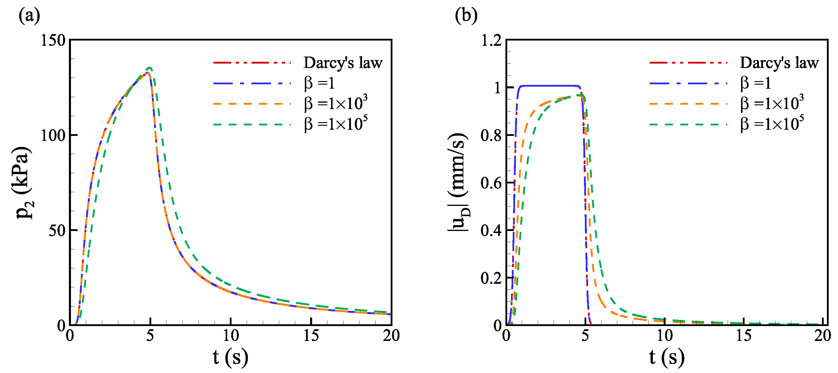
Interstitial fluid pressure plays a crucial role in governing the convective transport and absorption of drug molecules in the tissue. An approximate continuum poroelasticity model is developed to mimic the pressure build-up and relaxation by introducing the time variation of pressure. The effects of elasticity, porosity, and permeability on pressure evolution are investigated after validating the proposed poroelastic model with the analytical solution and previous computational model. The advantage of this model lies in the simplicity of implementation while maintaining good accuracy in capturing the evolution of the interstitial pressure. The small elasticity of the tissue slows down the relaxation of pressure and lowers the magnitude of pressure, while the magnitude of pressure increases dramatically with decreasing hydraulic permeability. Pressure evolution for low hydraulic permeability tends to be more sensitive to small elasticity, i.e., the relaxation time is longer for low hydraulic permeability at the same elasticity. The effect of variable porosity-dependent permeability is found to alleviate the high pressure due to increased porosity and permeability near the injection site.

To better address the microscopic structure of the lymphatic vessel membrane, an improved Kedem–Katchalsky model is developed for solute transport across the explicit vessel wall. The transport and lymphatic uptake of drug solutes in a multi-layered medium are investigated to elucidate the effect of heterogeneity of multi-layered structure and the heterogeneous vessel network. We investigate the convective diffusion of various macromolecules through the hybrid lymphatic vessel network by varying the Stokes radius and solute diffusivity across the opening lymphatic valves. With a smaller Stokes radius and larger solute diffusivity, the lymphatic uptake is significantly fast. Finally, the effect of the lymphatic vessel network structure is investigated through the fractal trees and Voronoi structures. We find that the Voronoi structure in the subcutaneous layer is more efficient in drug absorption because there are more interactions between the drug molecules and the vessel surfaces in the dermis and hypodermis layers.

For future work, the computational model can be further coupled with the mathematical model for the lymph flow inside the lymphatic vessels. In this way, the effect of the lymph flow rate can be incorporated into the model. The computational models developed here can also be coupled with the pharmacokinetic (PK) models to better predict drug bioavailability.

References

1. Swartz, M.A. The physiology of the lymphatic system. Adv. Drug Deliv. Rev. 2001, 50, 3–20. [Google Scholar] [CrossRef] [PubMed]
2. Moore, J.E.; Bertram, C.D. Lymphatic System Flows. Annu. Rev. Fluid Mech. 2018, 50, 459–482. [Google Scholar] [CrossRef] [PubMed]
3. Breslin, J.W.; Yang, Y.; Scallan, J.P.; Sweat, R.S.; Adderley, S.P.; Murfee, W.L. Lymphatic Vessel Network Structure and Physiology. Compr. Physiol. 2018, 12, 207–299. [Google Scholar] [CrossRef]
4. Oliver, G.; Kipnis, J.; Randolph, G.J.; Harvey, N.L. The Lymphatic Vasculature in the 21st Century: Novel Functional Roles in Homeostasis and Disease. Cell 2020, 182, 270–296. [Google Scholar] [CrossRef]
5. Swartz, M.A.; Kaipainen, A.; Netti, P.A.; Brekken, C.; Boucher, Y.; Grodzinsky, A.J.; Jain, R.K. Mechanics of interstitial-lymphatic fluid transport: Theoretical foundation and experimental validation. J. Biomech. 1999, 32, 1297–1307. [Google Scholar] [CrossRef]
6. Viola, M.; Sequeira, J.; Seiça, R.; Veiga, F.; Serra, J.; Santos, A.C.; Ribeiro, A.J. Subcutaneous delivery of monoclonal antibodies: How do we get there? J. Control Release 2018, 286, 301–314. [Google Scholar] [CrossRef]
7. McDonald, T.A.; Zepeda, M.L.; Tomlinson, M.J.; Bee, W.H.; Ivens, I.A. Subcutaneous administration of biotherapeutics: Current experience in animal models. Curr. Opin. Mol. Ther. 2010, 12, 461–470. [Google Scholar]
8. Dychter, S.S.; Gold, D.A.; Haller, M.F. Subcutaneous drug delivery: A route to increased safety, patient satisfaction, and reduced costs. J. Infus. Nurs. 2012, 35, 154–160. [Google Scholar] [CrossRef]
9. Reichert, J.M. Marketed therapeutic antibodies compendium. In Proceedings of the MAbs, Valencia, Spain, 4–8 June 2012; Taylor & Francis: Abingdon, UK, 2012; Volume 4, pp. 413–415. [Google Scholar]
10. Wang, S.S.; Yan, Y.S.; Ho, K. US FDA-approved therapeutic antibodies with high-concentration formulation: Summaries and perspectives. Antib. Ther. 2021, 4, 262–272. [Google Scholar] [CrossRef]
11. Han, D.; Rahimi, E.; Aramideh, S.; Ardekani, A.M. Transport and Lymphatic Uptake of Biotherapeutics Through Subcutaneous Injection. J. Pharm. Sci. 2022, 111, 752–768. [Google Scholar] [CrossRef]
12. Rahimi, E.; Aramideh, S.; Han, D.; Gomez, H.; Ardekani, A.M. Transport and lymphatic uptake of monoclonal antibodies after subcutaneous injection. Microvasc. Res. 2022, 139, 104228. [Google Scholar] [CrossRef]
13. Han, D.; Li, C.; Araimdeh, S.; Sree, V.; Rahimi, E.; Tepole, A.B.; Ardekani, A.M. Lymphatic uptake of biotherapeutics through a 3D hybrid discrete-continuum vessel network in the skin tissue. J. Control Release 2023, 354, 869–888. [Google Scholar] [CrossRef] [PubMed]
14. de Lucio, M.; Bures, M.; Ardekani, A.M.; Vlachos, P.P.; Gomez, H. Isogeometric analysis of subcutaneous injection of monoclonal antibodies. Comput. Methods Appl. Mech. Eng. 2021, 373, 113550. [Google Scholar] [CrossRef]
15. Thomsen, M.; Hernandez-Garcia, A.; Mathiesen, J.; Poulsen, M.; Sørensen, D.N.; Tarnow, L.; Feidenhans, R. Model study of the pressure build-up during subcutaneous injection. PLoS ONE 2014, 9, e104054. [Google Scholar] [CrossRef] [PubMed] [Green Version]
16. Daugherty, A.L.; Mrsny, R.J. Formulation and delivery issues for monoclonal antibody therapeutics. Adv. Drug Deliv. Rev. 2006, 58, 686–706. [Google Scholar] [CrossRef] [PubMed]
17. Doughty, D.V.; Clawson, C.Z.; Lambert, W.; Subramony, J.A. Understanding subcutaneous tissue pressure for engineering injection devices for large-volume protein delivery. J. Pharm. Sci. 2016, 105, 2105–2113. [Google Scholar] [CrossRef]
18. Kim, H.; Park, H.; Lee, S.J. Effective method for drug injection into subcutaneous tissue. Sci. Rep. 2017, 7, 9613. [Google Scholar] [CrossRef] [Green Version]
19. Speziale, S.; Tenti, G.; Sivaloganathan, S. A poroelastic model of transcapillary flow in normal tissue. Microvasc. Res. 2008, 75, 285–295. [Google Scholar] [CrossRef]
20. Sachs, D.; Wahlsten, A.; Kozerke, S.; Restivo, G.; Mazza, E. A biphasic multilayer computational model of human skin. Biomech. Model. Mechanobiol. 2021, 20, 969–982. [Google Scholar] [CrossRef] [PubMed]
21. Leiderman, R.; Barbone, P.E.; Oberai, A.A.; Bamber, J.C. Coupling between elastic strain and interstitial fluid flow: Ramifications for poroelastic imaging. Phys. Med. Biol. 2006, 51, 6291–6313. [Google Scholar] [CrossRef]
22. Leng, Y.; Wang, H.; de Lucio, M.; Gomez, H. Mixed-dimensional multi-scale poroelastic modeling of adipose tissue for subcutaneous injection. Biomech. Model. Mechanobiol. 2022, 21, 1825–1840. [Google Scholar] [CrossRef] [PubMed]
23. Taylor, D.G.; Bert, J.L.; Bowen, B.D. A mathematical model of interstitial transport: II. Microvascular exchange in mesentery. Microvasc. Res. 1990, 39, 279–306. [Google Scholar] [CrossRef]
24. MacMinn, C.W.; Dufresne, E.R.; Wettlaufer, J.S. Large deformations of a soft porous material. Phys. Rev. Appl. 2016, 5, 044020. [Google Scholar] [CrossRef] [Green Version]
25. Akalp, U.; Bryant, S.J.; Vernerey, F.J. Tuning tissue growth with scaffold degradation in enzyme-sensitive hydrogels: A mathematical model. Soft Matter 2016, 12, 752–755. [Google Scholar] [CrossRef] [Green Version]
26. Li, Z.; Biswas, A.; Finkelstein, J.; Grein, S.; Kapoor, Y.; Milewski, M.; Queisser, G. Modeling Drug Absorption from the Dermis after an Injection. J. Pharm. Sci. 2021, 110, 1279–1291.e1. [Google Scholar] [CrossRef]
27. Ibrahim, R.; Nitsche, J.M.; Kasting, G.B. Dermal Clearance Model for Epidermal Bioavailability Calculations. J. Pharm. Sci. 2012, 101, 2094–2108. [Google Scholar] [CrossRef]
28. Kampmeier, O.F. The genetic history of the valves in the lymphatic system of man. Am. J. Anat. 1928, 40, 413–457. [Google Scholar] [CrossRef]
29. Suami, H.; Scaglioni, M. Anatomy of the Lymphatic System and the Lymphosome Concept with Reference to Lymphedema. Semin. Plast. Surg. 2018, 32, 005–011. [Google Scholar] [CrossRef]
30. Deegan, A.J.; Wang, R.K. Microvascular imaging of the skin. Phys. Med. Biol. 2019, 64, 07TR01. [Google Scholar] [CrossRef]
31. Ulvmar, M.H.; Mäkinen, T. Heterogeneity in the lymphatic vascular system and its origin. Cardiovasc. Res. 2016, 111, 310–321. [Google Scholar] [CrossRef] [Green Version]
32. Biot, M.A. General Theory of Three - Dimensional Consolidation. J. Appl. Phys. 1941, 12, 155–164. [Google Scholar] [CrossRef]
33. Biot, M.A. Mechanics of Deformation and Acoustic Propagation in Porous Media. J. Appl. Phys. 1962, 33, 1482–1498. [Google Scholar] [CrossRef]
34. Biot, M.A.; Temple, G. Theory of Finite Deformations of Porous Solids. Indiana Univ. Math. J. 1972, 21, 597–620. [Google Scholar] [CrossRef]
35. Coussy, O. Poromechanics; John Wiley & Sons: Hoboken, NJ, USA, 2004. [Google Scholar]
36. Taylor, D.G.; Bert, J.L.; Bowen, B.D. A mathematical model of interstitial transport: I. Theory. Microvasc. Res. 1990, 39, 253–278. [Google Scholar] [CrossRef]
37. Steuperaert, M.; Falvo D’Urso Labate, G.; Debbaut, C.; De Wever, O.; Vanhove, C.; Ceelen, W.; Segers, P. Mathematical modeling of intraperitoneal drug delivery: Simulation of drug distribution in a single tumor nodule. Drug Deliv. 2017, 24, 491–501. [Google Scholar] [CrossRef] [Green Version]
38. Baxter, L.T.; Jain, R.K. Transport of fluid and macromolecules in tumors. I. Role of interstitial pressure and convection. Microvasc. Res. 1989, 37, 77–104. [Google Scholar] [CrossRef]
39. Teo, C.S.; Tan, W.H.K.; Lee, T.; Wang, C. Transient interstitial fluid flow in brain tumors: Effect on drug delivery. Chem. Eng. Sci. 2005, 60, 4803–4821. [Google Scholar] [CrossRef]
40. Moghadam, M.C.; Deyranlou, A.; Sharifi, A.; Niazmand, H. Numerical simulation of the tumor interstitial fluid transport: Consideration of drug delivery mechanism. Microvasc. Res. 2015, 101, 62–71. [Google Scholar] [CrossRef]
41. Biot, M.A. The elastic coefficients of the theory of consolidation. J. Appl. Mech. 1957, 24, 594–601. [Google Scholar] [CrossRef]
42. Sefidgar, M.; Soltani, M.; Raahemifar, K.; Sadeghi, M.; Bazmara, H.; Bazargan, M.; Naeenian, M.M. Numerical modeling of drug delivery in a dynamic solid tumor microvasculature. Microvasc. Res. 2015, 99, 43–56. [Google Scholar] [CrossRef]
43. Pishko, G.L.; Astary, G.W.; Mareci, T.H.; Sarntinoranont, M. Sensitivity analysis of an image-based solid tumor computational model with heterogeneous vasculature and porosity. Ann. Biomed. Eng. 2011, 39, 2360. [Google Scholar] [CrossRef] [Green Version]
44. Heppell, C.; Roose, T.; Richardson, G. A Model for Interstitial Drainage Through a Sliding Lymphatic Valve. Bull. Math. Biol. 2015, 77, 1101–1131. [Google Scholar] [CrossRef] [Green Version]
45. Adamson, R. Microvascular Endothelial Cell Shape and Size in Situ. Microvasc. Res. 1993, 46, 77–88. [Google Scholar] [CrossRef]
46. Michel, C.C.; Curry, F.E. Microvascular Permeability. Physiol. Rev. 1999, 79, 703–761. [Google Scholar] [CrossRef] [Green Version]
47. Armstrong, J.K.; Wenby, R.B.; Meiselman, H.J.; Fisher, T.C. The hydrodynamic radii of macromolecules and their effect on red blood cell aggregation. Biophys. J. 2004, 87, 4259–4270. [Google Scholar] [CrossRef] [Green Version]
48. Han, D. Quantitative Investigation of Transport and Lymphatic Uptake of Biotherapeutics through Three-Dimensional Physics-Based Computational Modeling. Ph.D. Thesis, Purdue University Graduate School, West Lafayette, IN, USA, 2023. [Google Scholar]
49. Gibney, M.A.; Arce, C.H.; Byron, K.J.; Hirsch, L.J. Skin and subcutaneous adipose layer thickness in adults with diabetes at sites used for insulin injections: Implications for needle length recommendations. Curr. Med. Res. Opin. 2010, 26, 1519–1530. [Google Scholar] [CrossRef]
50. Baxter, L.T.; Jain, R.K. Transport of fluid and macromolecules in tumors. II. Role of heterogeneous perfusion and lymphatics. Microvasc. Res. 1990, 40, 246–263. [Google Scholar] [CrossRef]
51. Baxter, L.T.; Jain, R.K. Transport of fluid and macromolecules in tumors: III. Role of binding and metabolism. Microvasc. Res. 1991, 41, 5–23. [Google Scholar] [CrossRef]
52. d’Esposito, A.; Sweeney, P.W.; Ali, M.; Saleh, M.; Ramasawmy, R.; Roberts, T.A.; Agliardi, G.; Desjardins, A.; Lythgoe, M.F.; Pedley, R.B.; et al. Computational fluid dynamics with imaging of cleared tissue and of in vivo perfusion predicts drug uptake and treatment responses in tumours. Nat. Biomed. Eng. 2018, 2, 773–787. [Google Scholar] [CrossRef] [Green Version]
53. Kalra, A.; Lowe, A. An Overview of Factors Affecting the Skins Youngs Modulus. J. Aging Sci. 2016, 4, 1000156. [Google Scholar] [CrossRef]
54. van Kuilenburg, J.; Masen, M.A.; van Der Heide, E. Contact modelling of human skin: What value to use for the modulus of elasticity? Proc. Inst. Mech. Eng. Part J Eng. Tribol. 2013, 227, 349–361. [Google Scholar] [CrossRef] [Green Version]
55. Zakaria El-R, J.; Lofthouse, M.F.; Flessner, M.F. In vivo hydraulic conductivity of muscle: Effects of hydrostatic pressure. Am. J. Physiol. 1997, 273, H2774. [Google Scholar] [CrossRef]
56. González-Suárez, A.; Gutierrez-Herrera, E.; Berjano, E.; Jimenez Lozano, J.N.; Franco, W. Thermal and elastic response of subcutaneous tissue with different fibrous septa architectures to RF heating: Numerical study. Lasers Surg. Med. 2015, 47, 183–195. [Google Scholar] [CrossRef]
57. Swartz, M.A.; Fleury, M.E. Interstitial flow and its effects in soft tissues. Annu. Rev. Biomed. Eng. 2007, 9, 229. [Google Scholar] [CrossRef] [Green Version]
58. Levick, J.R. Flow through interstitium and other fibrous matrices. Q. J. Exp. Physiol. 1987, 72, 409–437. [Google Scholar] [CrossRef]
59. Oftadeh, R.; Connizzo, B.K.; Nia, H.T.; Ortiz, C.; Grodzinsky, A.J. Biological connective tissues exhibit viscoelastic and poroelastic behavior at different frequency regimes: Application to tendon and skin biophysics. Acta Biomater. 2018, 70, 249–259. [Google Scholar] [CrossRef]
60. Barry, S.I.; Aldis, G.K. Comparison of models for flow induced deformation of soft biological tissue. J. Biomech. 1990, 23, 647–654. [Google Scholar] [CrossRef]
61. Salathe, E.P.; An, K. A mathematical analysis of fluid movement across capillary walls. Microvasc. Res. 1976, 11, 1–23. [Google Scholar] [CrossRef]
62. DuFort, C.; DelGiorno, K.; Carlson, M.; Osgood, R.; Zhao, C.; Huang, Z.; Thompson, C.; Connor, R.; Thanos, C.; Scott Brockenbrough, J.; et al. Interstitial Pressure in Pancreatic Ductal Adenocarcinoma Is Dominated by a Gel-Fluid Phase. Biophys. J. 2016, 110, 2106–2119. [Google Scholar] [CrossRef] [Green Version]
63. Ozerdem, U. Measuring interstitial fluid pressure with fiberoptic pressure transducers. Microvasc. Res. 2009, 77, 226–229. [Google Scholar] [CrossRef] [Green Version]
64. Zhao, H.; Graf, O.; Milovic, N.; Luan, X.; Bluemel, M.; Smolny, M.; Forrer, K. Formulation development of antibodies using robotic system and high-throughput laboratory (HTL). J. Pharm. Sci. 2010, 99, 2279–2294. [Google Scholar] [CrossRef]
65. Chary, S.R.; Jain, R.K. Direct measurement of interstitial convection and diffusion of albumin in normal and neoplastic tissues by fluorescence photobleaching. Proc. Natl. Acad. Sci. USA 1989, 86, 5385–5389. [Google Scholar] [CrossRef] [Green Version]
66. Ryan, T.J. Structure and Function of Lymphatics. J. Investig. Dermatol. 1989, 93, S18–S24. [Google Scholar] [CrossRef]
67. Sree, V.D.; Rausch, M.K.; Tepole, A.B. Linking microvascular collapse to tissue hypoxia in a multiscale model of pressure ulcer initiation. Biomech. Model. Mechanobiol. 2019, 18, 1947–1964. [Google Scholar] [CrossRef]
68. Roose, T.; Swartz, M.A. Multiscale modeling of lymphatic drainage from tissues using homogenization theory. J. Biomech. 2011, 45, 107–115. [Google Scholar] [CrossRef]
69. Rathore, N.; Pranay, P.; Bernacki, J.; Bruce, E.; Ji, W.; Walls, E. Characterization of protein rheology and delivery forces for combination products. J. Pharm. Sci. 2012, 101, 4472–4480. [Google Scholar] [CrossRef]
70. Khaled, A.R.; Vafai, K. The role of porous media in modeling flow and heat transfer in biological tissues. Int. J. Heat Mass Transf. 2003, 46, 4989–5003. [Google Scholar] [CrossRef]
71. Beavers, G.S.; Joseph, D.D. Boundary conditions at a naturally permeable wall. J. Fluid Mech. 1967, 30, 197–207. [Google Scholar] [CrossRef]
72. Le Reun, T.; Hewitt, D.R. High-Rayleigh-number convection in porous-fluid layers. J. Fluid Mech. 2021, 920, A35. [Google Scholar] [CrossRef]
73. Beavers, G.S.; Sparrow, E.M. Non-Darcy Flow Through Fibrous Porous Media. J. Appl. Mech. 1969, 36, 711–714. [Google Scholar] [CrossRef]
Figure 1. Illustration of a small branch of initial lymphatics.
Biology 12 00942 g001
Figure 2. Conceptual overview of the physics-based computational models for lymphatic uptake in soft skin tissue through subcutaneous injection.
Biology 12 00942 g002
Figure 3. Time evolution of (a) interstitial fluid pressure p 2 , (b) magnitude of Darcy velocity | u D | , at the point P 2 , 10 mm below the injection point, for various elastic modules E. For a rigid porous medium modeled by Darcy’s law E .
Biology 12 00942 g003
Figure 4. Time evolution of interstitial fluid pressure at (a) the injection point P 0 , (b) point 2 mm below the injection point P 1 , (c) point 10 mm below the injection point P 2 , along the symmetric axis of the domain (center line), for various hydraulic permeability k. The elastic modulus E = 80 kPa.
Biology 12 00942 g004
Figure 5. Time evolution of (a) interstitial fluid pressure p 2 and (b) magnitude of Darcy velocity | u D | for variable permeability compared to constant permeability. The pressure and velocity are results at the point P 2 , 10 mm below the injection point. The initial porosity ε = 0.01 and elasticity E v = 80 kPa.
Biology 12 00942 g005
Figure 6. Distribution of (a) interstitial fluid pressure p with values in unit of kPa , (b) porosity, (c) hydraulic permeability with values in unit of 10 13   m 2 at the end of injection t = 5.0 s in the single-layered domain with variable porosity and permeability. The initial porosity, ε 0 = 0.01 , and permeability, k 0 = 1 × 10 13 m 2 .
Biology 12 00942 g006
Figure 7. Distribution of (a) interstitial fluid pressure p with values in unit of kPa , (b) Péclet number P e and (c) lymphatic drainage ϕ l with values in unit of 10 6 s 1 , in a multi-layered domain at t = 5 s , 20 s , 60 s .
Biology 12 00942 g007
Figure 8. Vessel network of blood (in red) and lymphatic capillaries (in green).
Biology 12 00942 g008
Figure 9. (a) Time evolution of drug percentage in the tissue (solute volume normalized with the initial injection volume) for various Stokes radius r s and solute diffusivity across the discrete lymphatic vessel wall. (b) Time evolution of interstitial fluid pressure p 0 (the injection point), p 1 (2 mm above the injection point), and p 2 (5 mm below the injection point) at three different points along the symmetric axis of the domain for the baseline case ( R s = 5 nm ).
Biology 12 00942 g009
Figure 10. Lymphatic vessel networks with different structures: (a) fractal trees, (b) Voronoi structure.
Biology 12 00942 g010
Figure 11. Comparison of drug evolution in the tissue with two different lymphatic vessel network structures.
Biology 12 00942 g011
Figure 12. Comparison of drug distribution in multi-layered skin tissue with two different structures, (a) fractal trees, (b) Voronoi structure, at t = 300 s.
Biology 12 00942 g012