Article

Is It Better for a Publisher to Release an Audiobook after Its E-Book Version?

School of Business, Hubei University, Wuhan 430062, China
Systems 2024, 12(1), 33; https://doi.org/10.3390/systems12010033
Submission received: 11 December 2023 / Revised: 16 January 2024 / Accepted: 17 January 2024 / Published: 18 January 2024
(This article belongs to the Section Systems Practice in Social Science)

Abstract

:
The e-books industry is mature, and audiobooks are becoming increasingly popular. More and more publishers are coming to realize that audiobooks could be a potential revenue driver and intend to release audiobooks. Considering that there is a certain substitutability between e-books and audiobooks, publishers need to decide how to release a book in its audible version and its e-book version into the market. In this paper, we incorporate the discount factor and the consumers’ acceptance level for audiobooks into the consumer utility by dividing consumers into two types, high-value type and low-value type, and construct two different release models: releasing the audiobook and the e-book simultaneously and releasing the audiobook after the e-book. Using an optimization tool, we investigate pricing strategies of a monopolistic publisher under two different release models. By comparing the theoretical results of the two models, we find that when the consumers’ patience exceeds a certain threshold, releasing a book in its audible version after its e-book version is better for the publisher, and the publisher should adopt a skimming (refers to decreasing markups over time) pricing strategy for the e-book in this case. Further, the publisher should set a higher price for the audiobook than the e-book, whether or not they release the audiobook after the e-book. In addition, we conduct a numerical analysis to investigate how the discount factor, the percentage of high-value consumers, and the high-value consumers’ acceptance level for audiobooks affect the consumer surplus and the social welfare. This study offers publishers some managerial insights into the complex issues involving pricing and release strategies.

1. Introduction

As smartphones, and now intelligent, mini, and portable speakers, reinvent the way we live, along with the global outbreak of COVID-19 in 2019, listening to books is growing in popularity as more people are discovering the convenience and pleasure of them. According to the results from the Audio Publishers Association’s annual sales survey, released on 7 June 2022 [1], U.S. audiobook sales in 2021 amounted to USD 1.6 billion, up 25% from the previous year, and this continues the ten-year trend of double-digit revenue growth. Audiobooks are attracting more consumers, no publisher wants to miss tremendous growth opportunities on audiobooks. However, audiobooks can substitute e-books to some extent, since they deliver the same context to consumers. E-book sales peaked in 2014 but after the peak in 2014 began to fall. According to a market research report released by IBISWorld on 21 April 2022 [2], e-book sales have declined sharply over the eight years to 2022 after explosive growth in the 2000s and early 2010s.
Publishers have to take into account the impact of audiobooks on e-books. In particular, now the e-books industry is mature, leaving an opportunity for audiobooks to balance publishers’ profit, many publishers are considering how to release a book in its audible version and its e-book version. From Amazon.com, we can find that there are some books where their two versions were simultaneously released. For example, for one of the bestsellers on Amazon.com, «Everything Is F*cked: A Book About Hope», its Kindle edition and audible edition were simultaneously released on 14 May 2019. The Kindle edition and audiobook of Michelle Obama’s book «Becoming» were simultaneously released on 13 November 2018. For the book «Fear: Trump in the White House» by Bob Woodward, which is also on Amazon’s bestsellers list, its Kindle edition and audible edition were simultaneously released on 11 September 2018. However, from Amazon.com, we can also find that some books with Kindle editions were released first and then their audible editions were released into the market. For example, the Kindle edition of the classic novel «Don Quixote» was released on 29 January 2009, then its audible book was released on 29 October 2012. For the French children’s book «The Little Prince», its Kindle edition was first released on 19 May 2018, then its audible version was released on 23 May 2020. In addition, from Amazon’s site, it can also be seen that nearly all audible versions of books on Amazon are more expensive than their Kindle editions; see the book example shown in Figure 1. Figure 1 illustrates an example of retail prices from a top-ranked bestseller in Audible Books & Originals on Amazon.com. The audible version of the book is sold at about USD 29.93, but the retail price of the Kindle edition is USD 14.99.
This motivates our research questions: How does the publisher choose the right sequence of releasing audiobooks and e-books? Specifically, under what circumstances should a publisher release an audiobook after its e-book version? Or under what circumstances should a publisher release the audiobook and its e-book version simultaneously? If the publisher releases the audiobook after its e-book version, some impatient consumers, who originally intended to buy the audiobook, may turn to the e-book, and that may soften the impact of audiobooks on e-books. On the other hand, some patient consumers may choose to wait until the audiobook is released. But as time goes on, the consumers’ valuation for the book will fall if the audiobook is released after the e-book. How should the publisher could weigh these factors to make the optimal choice by setting the right price for the audiobook and the e-book? In addition, why are audiobooks more expensive than e-books? This research investigates these questions.
This paper is intended to present analyses of a monopolistic publisher’s decision about how to release e-books and audiobooks, and corresponding pricing strategies, using mathematical modeling. Specifically, we consider two release models, namely, one model under which the publisher releases a book in its audible version and its e-book version simultaneously, and the other model under which the audible version is released after the e-book version. We incorporate three important factors into our models: the discount factor, the consumers’ acceptance level for audiobooks, and the percentage of high-value consumers. By comparing the profits of the two different release models, we study the conditions in which the publisher decides which model to use, and the corresponding optimal pricing for the audiobook and the e-book. In addition, we analyze how the above three factors affect the publisher’s optimal choice, the consumer surplus, as well as social welfare.
The rest of this paper is organized as follows: we review related work in Section 2. In Section 3, we deduce the demand functions of the audiobook and the e-book under two different release models based on the consumer utility theory. Section 4 proposes corresponding decision problems of the publisher under two different release models, and analyzes the publisher’s optimal choice by solving two decision models. In Section 5, we evaluate the effects of various factors on the consumer surplus and social welfare using a numerical analysis. Section 6 discusses our main results and gives corresponding managerial implications. Finally, Section 7 concludes our study and indicates possible future extensions of this paper.

2. Literature Review

Since both e-books and audiobooks are digital products, we first review the literature related to digital products in Section 2.1. Then, we concentrate on reviewing the literature related to the book industry in Section 2.2. Finally, we summarize our contributions in Section 2.3.

2.1. Literature Related to Digital Products

Among the literature related to digital products, most studies put piracy and pricing together to analyze the optimal strategies for firms. Ref. [3] investigates how the government’s policy on punishing piracy and subsidizing legal products, and a monopolist’s pricing strategies affect social welfare. Ref. [4] focuses on analyzing how a firm sets optimal prices and the right DRM (i.e., digital rights management) protection level for the legal product. The results show that a lower DRM protection level is better for the firm if it can enforce price discrimination. Ref. [5] studies how piracy affects the firm’s profit, and strategies on pricing and quality choice. Ref. [6] also studies how piracy affects the pricing policies of producers in the music industry based on an approximate and cumulative demand function. They show that piracy may lead to a higher price for legal music products. Refs. [7,8] investigate how piracy affects the pricing and development strategies of a software firm. Ref. [9] uses a comparative case study to analyze digital business model responses of some industries most affected by piracy, and examines the characteristics of digital piracy. Ref. [10] considers how firms’ DRM limit on legal products and government’s enforcement on pirated products affect the optimal pricing and DRM protection level of the firm. Ref. [11] investigates how piracy affects a firm’s decision on the quality of digital products using a game approach. Ref. [12] investigates how piracy affects the bundling of a monopolist seller. The results show that piracy can severely diminish the appeal of bundling to the seller. Ref. [13] examines the pay-what-you-want (PWYW) pricing strategy in the presence of piracy. This study shows that it is optimal to eliminate piracy under certain conditions. Ref. [14] demonstrates the salience of explicit and implicit consumer attitudes in the presence of digital piracy. The results show that idealism has a negative effect on the explicit attitude but relativism has a positive effect on the explicit attitude.
There are also some studies centering on pricing strategies of digital products without taking into account piracy. For example, Ref. [15] analyzes how information goods firms set the optimal price for their products based on an incomplete information model. The results show that a fixed-fee pricing strategy may be optimal for firms under certain conditions. Refs. [16,17,18,19,20] analyze the equilibrium strategy of members using a game approach. Refs. [21,22] incorporate network effects into the models. They find the network effects play a key role. Ref. [23] analyzes how to concert the preference between physical and digital goods. The results show that digital goods are relatively preferred.

2.2. Literature Related to the Book Industry

Our study is closely related to the literature about digital products. Specifically, this study is more related to the literature that centers on the book industry.
There is some empirical research about the book industry. Ref. [24] analyzes how e-books and e-commerce affect the current book industry, and investigates the future evolution of the book industry, based on qualitative analysis. This study points out that printed books will not go away, but sellers should adjust development strategies of books to changing consumer preferences. Ref. [25] investigates the effects of e-books on the sales of printed books by comparing the data on bestsellers of printed books and e-books from Amazon. The results show that e-books are more likely to cannibalize the sale of printed books if the book is a hotseller. Ref. [26] also analyzes the impact of e-books on the book industry, the results show there is no obvious evidence to support the view that a rise in e-books results in a decline in individual booksellers. Ref. [27] analyzes how the U.S. online book retailers set prices for their products over the period of 2001–2006. The empirical results show that the evolving driving factors led to volatile prices over this period. Ref. [28] analyzes how e-books affect the sales of printed books using data from Amazon based on a natural experiment. The results indicate that printed books and e-books will not strongly cannibalize each other in the short term. By analyzing individual-level data from Amazon, Ref. [29] examines an intertemporal price discrimination strategy with e-books and complementary reading devices. The results indicate that firms should adopt an investing pricing strategy for e-books and a skimming pricing strategy for e-readers. Ref. [30] examines the antecedents of consumers’ intentions to adopt audiobook applications by integrating the decomposed theory of planned behavior (DTPB) with switching cost theory (SCT). This study presents some important factors in influencing consumers’ intentions to adopt audiobook applications.
In the literature related to the book industry, there are also a lot of studies that focus on analysis of pricing strategies by using game theoretical models. The agency model and the wholesale model are two prevailing pricing models in the book industry. In the agency model, suppliers (rather than retailers) set the final retail prices and sales revenue is split between suppliers and retailers according to endogenously determined shares. In the wholesale model, suppliers first offer products to retailers at wholesale prices, retailers then set retail prices to consumers. Ref. [31] uses a game theoretical model to study the pricing of e-books and e-readers in a two-echelon supply chain, which comprises a publisher and a retailer. By comparing the agency model and the wholesale model, they find that if the price of the printed books is given, the price of e-books in the agency model is higher than that in the wholesale model, but the price of e-readers is lower in the agency model. Ref. [32] uses a Stackelberg game to study the pricing of e-books and printed books. Similarly, by comparing two prevailing pricing models, this study shows that the agency model is superior to the wholesale model under most circumstances. Ref. [33] analyzes the equilibrium strategies of a publisher and a retailer in the context of an imperfect competition, by comparing two pricing models. The results show that under certain forms of demand function, the retailer can obtain more profit in the agency model, while the publisher can obtain more profit in the wholesale model. Unlike previous studies, the revenue sharing percentage under the agency model in this study is a variable, while this percentage in previous studies is exogenously fixed. Ref. [34] utilizes a game theory tool to compare the agency model and the wholesale model under decentralized and horizontally centralized channels. This study finds that in the decentralized channels, there is always a Pareto zone under the agency model; but only under certain conditions is a Pareto zone found in the horizontally centralized channels. Ref. [35] incorporates network externalities into e-book pricing models. By comparing two pricing models: the agency model and the wholesale model, this study finds that both the prices of e-books and printed books in the agency model are lower than those in the wholesale model.

2.3. Our Contributions to the Related Literature

Our study contributes to the related literature in the following ways. We develop demand functions that are specific to the e-book and audiobook markets. In this study, we use a consumer choice model which reflects the horizontal differentiation between e-books and audiobooks to deduce the demand functions of e-books and audiobooks under two different release models. Specifically, we incorporate three important factors into consumers’ utility function: consumers’ acceptance level for audiobooks, the percentage of high-value consumers, and the discount factor under the model where the audiobook is released after the e-book. By analyzing the optimal pricing strategies of the publisher and comparing the publisher’s profits under the two different release models, we study the conditions that determine which model the publisher should choose. We find the discount factor is a key factor in the publisher’s choice. If the discount factor is large enough, which means consumers have enough patience, then releasing the audiobook after the e-book is much better for the publisher; but if consumers are less patient, it is better for the publisher to release the audiobook and the e-book simultaneously.
Most studies on the book industry focus on e-books and physical books. To the best of our knowledge, this is the first work that focuses on audiobooks and e-books, and investigates the conditions under which publishers should release the audiobook after the e-book. Specifically, most related studies assume all consumers are of the same type. For example, Ref. [32] assumes all consumers’ acceptance levels for the digital product are greater than 1 or less than 1. The acceptance level for the digital product being greater than 1 means that the consumers prefer the digital version to the printed book. Unlike the existing related studies, we divide the consumers into two types: high-value type and low-value type. This is a more realistic assumption and is our main theoretical contribution to the existing literature. Our research also provides valuable insights to business managers involved in the book industry.

3. Model Development

We consider a monopolistic profit-maximizing publisher who plans to manufacture and sell a book with audible and e-book versions to consumers. The publisher needs to decide whether or not to release the book with the e-book and audible versions simultaneously to the market. Specifically, the publisher is faced with two choices: releasing a book with audible and e-book versions simultaneously, or releasing a book with the audible version after its e-book version. The publisher also needs to decide on the optimal prices of the different books.
Notably, both the audiobook and the e-book are digital products, while the printed book is a physical product. Both theoretical and technological developments of printed books are relatively mature. The interaction effects between e-books and printed books tend to be stable. The advent of audiobooks has a far greater influence on e-books than printed books. Moreover, in reality, some publications are only available digitally and there are no corresponding physical editions in a short run. For example, we can find that some books are only available in digital formats on Amazon’s U.S. site; and the development of the global network of literature is the concomitant of the new rise in digital media. Digital publishing is the first priority of online literature. Specifically, online literature publishers need to decide how to release e-book and audible versions of the content. Even if the publishers may release the printed book in the near future, the publishers’ priority is to decide how to release the e-book and audible versions in the short-run. Generally, whether the publishers will release the printed book depends on how the digital markets perform. Thus, for online publishers, releasing the printed version and releasing the digital version are not things to consider simultaneously. Thus, to concentrate our analysis on the competition between audiobooks and e-books, we do not involve printed books in our model.
To facilitate follow-up analysis and describe the publisher’s optimization problem, some notes and assumptions are first given in Section 3.1. Then, in Section 3.2 and Section 3.3, respectively, by analyzing a utility-based consumer choice model we deduce the demand functions of the audiobook and the e-book under two different release models.

3.1. Notation and Assumptions

Throughout this paper, we use the pronouns “he” and “she” to denote the publisher and a typical consumer, respectively. Consumers have heterogeneous preferences on the e-book. A consumer’s preference for the e-book is characterized by her valuation for the e-book v, which is uniformly distributed over [ 0 , 1 ] . To characterize the consumer’s preference for the audible version, we divide all consumers into two types: high-value type and low-value type, according to the consumers’ acceptance level for the audiobook. Specifically, we use θ H ( θ H > 1 ) and θ L ( θ L < 1 ) to denote high-value consumers and low-value consumers, respectively. Here, θ H denotes consumers who prefer the book in the audible version relative to its e-book version, whereas θ L denotes consumers who prefer the e-book version over the audible version. That is, high-value (low-value) consumers’ valuation for the audible version is v θ H ( v θ L ). Without loss of generality, we assume the percentage of high-value consumers is λ and the rest 1 λ of the consumers are low-value.
We use the symbol SR to denote the model where the publisher releases a book with the audible and e-book versions simultaneously, and use the symbol LR to denote the model where the publisher releases a book with the audible version after its e-book version. In the SR model, the consumer has three choices: buying the e-book, buying the audiobook, or buying nothing. The utility u e the consumer obtains from the e-book is v p e , where p e is the retail price of the e-book. The utility u a H the high-value consumer obtains from the audiobook is v θ H p a , and the utility u a L the low-value consumer obtains from the audiobook is v θ L p a , where p a is the retail price of the audiobook. If the consumer chooses not to buy any product, then her utility is 0.
In the LR model, there are two stages. In the first stage, the publisher releases only the e-book version. In the second stage, the publisher will release the book with the audible version, and both versions of the book are sold on the market in this stage. We use p e 1 to denote the retail price of the e-book in the first stage. To achieve the maximization of profit, the publisher will adjust the retail price of the e-book from p e 1 to p e 2 if the audiobook is released to the market, where p e 2 is the retail price of the e-book in the second stage. All high-value consumers make decisions after the audiobook is released in the second stage, that is, they do not buy anything in the first stage. However, in the first stage, a low-value consumer will buy the e-book if she can obtain a positive utility from the e-book with a retail price p e 1 . In the second stage, all consumers who do not buy anything in the first stage have three choices: buying the e-book, buying the audiobook, or buying nothing.
Moreover, we assume that the consumer’s valuation for the e-book will drop to δ v in the second stage, where δ ( 0 δ 1 ) is a discount factor. Here, the discount factor follows the definition in game theory [36]. The bigger the value of the discount factor, the more patient the consumer is. The utility u e 1 a consumer obtains from the e-book in the first stage is v p e 1 , the utility u e 2 a consumer obtains from the e-book in the second stage is δ v p e 2 . In the second stage, the utility u a H a high-value consumer obtains from the audiobook is δ v θ H p a , and the utility u a L a low-value consumer obtains from the audiobook is δ v θ L p a . If the consumer chooses not to buy any product, then her utility is 0.
Without loss of generality, we assume all of the aforementioned variables are between 0 and 1 expect θ H . Table 1 summarizes all the notation referred to in this model.

3.2. Demand Analysis for E-Book and Audiobook in SR Model

Considering the individual rationality (IR) constraint and the incentive compatibility (IC) constraint, the high-value consumer will choose to buy the e-book if and only if u e 0 and u e u a H ; she will choose to buy the audiobook if and only if u a H 0 and u a H u e ; otherwise, she will do nothing. Similarly, the low-value consumer will choose to buy the e-book if and only if u e 0 and u e u a L ; she will choose to buy the audiobook if and only if u a L 0 and u a L u e ; otherwise, she will do nothing.
According to these two constraints, we can, respectively, deduce the valuation threshold v ¯ H of the high-value consumer who is indifferent between buying the audiobook and the e-book, and the valuation threshold v ¯ L of the low-value consumer who is indifferent between buying the audiobook and the e-book. Specifically, these thresholds are, respectively, as follows: v ¯ H = p a p e θ H 1 , v ¯ L = p e p a 1 θ L . There are u e 0 and u e u a H if and only if v p e and v v ¯ H ; u a H 0 and u a H u e if and only if v p a θ H and v v ¯ H ; u e 0 and u e u a L if and only if v p e and v v ¯ L ; u a L 0 and u a L u e if and only if v p a θ L and v v ¯ L .
By analysis, we can derive the demand functions of the e-book and the audiobook as follows. The detailed derivation can be found in Appendix A.
D e = ( 1 λ ) ( 1 p e ) + λ ( p a p e θ H 1 p e ) p a θ H p e ( 1 λ ) ( 1 p e ) θ L p e p a θ H p e ( 1 λ ) ( 1 p e p a 1 θ L ) p a θ L p e
D a = λ ( 1 p a p e θ H 1 ) p a θ H p e λ ( 1 p a θ H ) θ L p e p a θ H p e λ ( 1 p a θ H ) + ( 1 λ ) ( p e p a 1 θ L p a θ L ) p a θ L p e

3.3. Demand Analysis for E-Book and Audiobook in LR Model

In the LR model, there are two stages. In the first stage, there is only the e-book to be sold in the market. Specifically, a low-value consumer will buy the e-book if she can obtain a positive utility from the e-book, but no high-value consumers make a decision in this stage. In the second stage, the publisher releases the book with the audible version to the market. In this stage, those low-value consumers who did not buy the e-book in the first stage and all high-value consumers will make their decisions from the following three choices: buying the e-book, buying the audiobook, or doing nothing.
Considering the individual rationality (IR) constraint and the incentive compatibility (IC) constraint, the low-value consumer will choose to buy the e-book if and only if u e 1 0 in the first stage. That is, low-value consumers in the interval [ p e 1 , 1 ] will buy the e-book in the first stage, others wait for entering the second stage. Thus, the demand for the e-book in the first stage is as follows:
D e 1 = ( 1 λ ) ( 1 p e 1 )
The low-value consumers whose valuations are less than p e 1 and all high-value consumers enter the second stage. Further, in the second stage, a low-value consumer who does not buy the e-book in the first stage will buy the e-book if and only if u e 2 0 and u e 2 u a L ; she will choose to buy the audiobook if and only if u a L 0 and u a L u e 2 ; otherwise, she will choose to do nothing. Similarly, the high-value consumer will choose to buy the e-book if and only if u e 2 0 and u e 2 u a H ; she will choose to buy the audiobook if and only if u a H 0 and u a H u e 2 ; otherwise, she will choose to do nothing.
According to the above two constraints, we can, respectively, derive the valuation threshold v ¯ L 2 of the low-value consumer who is indifferent between buying the audiobook and the e-book in the second stage under the LR model, and the valuation threshold v ¯ H 2 of the high-value consumer who is indifferent between buying the audiobook and the e-book in the second stage under the LR model. Specifically, these thresholds are, respectively, as follows: v ¯ L 2 = p e 2 p a δ ( 1 θ L ) , v ¯ H 2 = p a p e 2 δ ( θ H 1 ) .
Similarly, we can, respectively, derive the demand for the e-book and the audiobook in the second stage as follows. See Appendix B for a detailed derivation.
(1)
If p e 2 δ p e 1 , there are
D e 2 = ( 1 λ ) ( p e 1 p e 2 δ ) + λ ( 1 p e 2 δ ) p a p e 2 + δ ( θ H 1 ) ( 1 λ ) ( p e 1 p e 2 δ ) + λ ( v ¯ H 2 p e 2 δ ) θ H p e 2 p a p e 2 + δ ( θ H 1 ) ( 1 λ ) ( p e 1 p e 2 δ ) θ L p e 2 p a θ H p e 2 ( 1 λ ) ( p e 1 v ¯ L 2 ) p e 2 δ ( 1 θ L ) p e 1 p a θ L p e 2 0 p a p e 2 δ ( 1 θ L ) p e 1
D a = 0 p a p e 2 + δ ( θ H 1 ) λ ( 1 v ¯ H 2 ) θ H p e 2 p a p e 2 + δ ( θ H 1 ) λ ( 1 p a δ θ H ) θ L p e 2 p a θ H p e 2 ( 1 λ ) ( v ¯ L 2 p a δ θ L ) + λ ( 1 p a δ θ H ) p e 2 δ ( 1 θ L ) p e 1 p a θ L p e 2 ( 1 λ ) ( p e 1 p a δ θ L ) + λ ( 1 p a δ θ H ) p a p e 2 δ ( 1 θ L ) p e 1
(2)
If δ p e 1 p e 2 δ , there are
D e 2 = λ ( 1 p e 2 δ ) p a p e 2 + δ ( θ H 1 ) λ ( v ¯ H 2 p e 2 δ ) θ H p e 2 p a p e 2 + δ ( θ H 1 ) 0 p a θ H p e 2
D a = 0 p a p e 2 + δ ( θ H 1 ) λ ( 1 v ¯ H 2 ) θ H p e 2 p a p e 2 + δ ( θ H 1 ) λ ( 1 p a δ θ H ) δ θ L p e 1 p a θ H p e 2 ( 1 λ ) ( p e 1 p a δ θ L ) + λ ( 1 p a δ θ H ) p a δ θ L p e 1
(3)
If δ p e 2 θ H θ L δ , there are:
D e 2 = 0
D a = 0 p a δ θ H λ ( 1 p a δ θ H ) δ θ L p e 1 p a δ θ H ( 1 λ ) ( p e 1 p a δ θ L ) + λ ( 1 p a δ θ H ) p a δ θ L p e 1
(4)
If p e 2 θ H θ L δ , there are
D e 2 = 0
D a = 0 p a δ θ H λ ( 1 p a δ θ H ) p a δ θ H

4. Strategy Analysis of Publisher

In this section, we will explore the optimal pricing strategy of the publisher under the SR model and the LR model by solving the publisher’s optimization problems. Then, by comparing the results of the two models, we will analyze which model the publisher should choose under which conditions.

4.1. Publisher’s Optimal Pricing Strategy under SR Model

In the SR model, the publisher releases a book in its e-book and audible versions to the market simultaneously. Since both e-books and audiobooks are digital products which can be reproduced at a negligible cost, we assume both the marginal costs of the e-book and the audiobook are zero. In addition, the production costs of digital products are mainly incurred in pre-production and the costs are usually sunk. Thus, the costs of the e-book and the audiobook are not involved in the model. The publisher needs to decide the retail prices of the e-book and the audiobook. Thus, the publisher’s optimization problem is as follows:
max p e , p a ( 0 , 1 ) π = p e D e + p a D a
where D e , D a are given in Section 3.2; please refer to Equations (1) and (2).
By solving the above optimization problem, we have the following theorem. The proof of this theorem and all the proofs of subsequent conclusions are available in Appendix D, Appendix E, Appendix F, Appendix G, Appendix H and Appendix I.
Theorem 1. 
If the publisher releases a book in its e-book and audible versions simultaneously to the market, the optimal prices of the e-book and the aduiobook, p e * , p a * , as well as the corresponding demand for the e-book and the audiobook, D e * , D a * , and the publisher’s total profit π * are, respectively, as follows:
p e * = 1 2 , p a * = θ H 2 , D e * = 1 λ 2 , D a * = λ 2 , π * = 1 + λ ( θ H 1 ) 4
From the above theorem, it can be seen that the publisher’s profit increases with the increasing percentage of high-value consumers. More high-value consumers means that there are more consumers that prefer the audiobook to the e-book. Increasing the proportion of high-value consumers will result in a decline in demand for the e-book, but a rise in sales of the audiobook. Further, from Theorem 1, it can be seen that the price of the audiobook is higher than that of the e-book. Thus, the profit increment of the audiobook can make up for the profit loss of the e-book, thereby boosting the publisher’s total profit. High-value consumers are the main force behind purchasing the audiobook. This result suggests that the publisher should devote himself to enhancing the percentage of high-value consumers if he plans to release the audiobook and the e-book simultaneously.
In addition, it can also be seen that the publisher’s profit increases with the increase in high-value consumers’ acceptance level for the audiobook. The main reason behind this it is that the publisher could set a higher price for the audiobook as high-value consumers’ acceptance level increases. However, the price of the e-book, and the demand for e-book and audiobook, are not affected by this acceptance level. Therefore, the publisher can benefit from a higher acceptance level of high-value consumers.

4.2. Publisher’s Optimal Pricing Strategy under LR Model

In the LR model, there are two stages. In the first stage, the publisher only releases the book in the e-book version to the market. He needs to decide the retail price of the e-book p e 1 . In the second stage, the publisher releases the book in the audible version to the market. He needs to decide the retail price of the audiobook p a and adjust the retail price of the e-book from p e 1 to p e 2 . The publisher’s profit function is as follows: π = p e 1 D e 1 + p e 2 D e 2 + p a D a , where D e 1 , D e 2 , and D a can be found in Section 3.3; please refer to Equations (3)–(11).
Using backward induction, we consider the publisher’s pricing model as the following three-step sequential decision:
Step 1. Given the price of the e-book in the first stage p e 1 , find the optimal pricing combination ( p e 2 ( p e 1 ) , p a ( p e 1 ) ) that maximizes the publisher’s profit π ( p e 1 , p e 2 , p a ) ;
Step 2. Find the optimal price of the e-book in the first stage p e 1 * that maximizes the publisher’s profit π ( p e 1 , p e 2 ( p e 1 ) , p a ( p e 1 ) ) ;
Step 3. Substituting the above p e 1 * back into the combination ( p e 2 ( p e 1 ) , p a ( p e 1 ) ) in step 1, the optimal price combination ( p e 2 * , p a * ) can be derived.
On the basis of the above steps and demand analysis under four cases in Section 3.3, we have the following conclusions after tedious mathematical derivation.
Lemma 1. 
When p e 2 δ p e 1 , the optimal prices of the e-book in the two stages p e 1 * , p e 2 * and the optimal price of the audiobook p a * , as well as the corresponding demand for the e-book and the audiobook, D e * , D a * , and the publisher’s optimal profit π * are, respectively, as follows:
p e 1 * = 2 + δ λ 4 δ ( 1 λ ) , p e 2 * = δ ( 1 + λ ) 4 δ ( 1 λ ) , p a * = δ θ H ( 4 δ ( 1 λ ) ) ( 1 λ ) ( 2 δ ) 2 ( 4 δ ( 1 λ ) ) , D e * = ( 1 λ ) ( 6 δ ( 2 λ ) ) 2 ( 4 δ ( 1 λ ) ) , D a * = λ 2 , π * = δ λ θ H ( 4 δ ( 1 λ ) ) + δ ( 1 λ ) + 4 ( 1 λ ) 4 ( 4 δ ( 1 λ ) ) .
Lemma 2. 
When δ p e 1 p e 2 δ , the optimal price of the e-book in the two stages p e 1 * , p e 2 * and the optimal price of the audiobook p a * , as well as the corresponding demand for the e-book and the audiobook, D e * , D a * , and the publisher’s optimal profit π * are, respectively, as follows:
(1) 
If λ θ L 4 θ H 3 θ L δ θ H θ L , there are p e 1 * = 1 2 , p e 2 * = δ 2 , p a * = δ θ H 2 , D e * = 1 λ 2 , D a * = λ 2 , π * = 1 λ + δ λ θ H 4 .
(2) 
If λ θ L 4 θ H 3 θ L δ θ H θ L , there are p e 1 * = 2 ( 1 λ ) θ H + λ θ L + δ λ θ H θ L 4 ( 1 λ ) θ H + λ θ L ( 1 λ ) δ θ H θ L , p e 2 * can be any value in the interval [ δ p e 1 * , δ ] , p a * = δ ( 1 + λ ) θ H θ L 4 ( 1 λ ) θ H + λ θ L ( 1 λ ) δ θ H θ L , D e * = ( 1 λ ) ( 2 ( 1 λ ) θ H + λ θ L + δ λ θ H θ L ) 2 ( 1 λ ) θ H + λ θ L δ θ H θ L ( 4 ( 1 λ ) θ H + λ θ L ( 1 λ ) δ θ H θ L ) 2 , D a * = ( 1 + λ ) ( ( 1 λ ) θ H + λ θ L ) 4 ( 1 λ ) θ H + λ θ L ( 1 λ ) δ θ H θ L , π * = ( 1 λ ) ( 1 λ ) θ H + λ θ L + δ λ θ H θ L 4 ( 1 λ ) θ H + λ θ L δ ( 1 λ ) θ H θ L .
Lemma 3. 
When δ p e 2 θ H θ L δ , the optimal price of the e-book in the two stages p e 1 * , p e 2 * and the optimal price of the audiobook p a * , as well as the corresponding demand for the e-book and the audiobook, D e * , D a * , and the publisher’s optimal profit π * are, respectively, as follows:
(1) 
If λ θ L 4 θ H 3 θ L δ θ H θ L , there are p e 1 * = 1 2 , p e 2 * can be any value in the interval [ δ , θ H θ L δ ] , p a * = δ θ H 2 , D e * = 1 λ 2 , D a * = λ 2 , π * = 1 λ + δ λ θ H 4 ;
(2) 
If λ θ L 4 θ H 3 θ L δ θ H θ L , there are p e 1 * = 2 ( 1 λ ) θ H + λ θ L + δ λ θ H θ L 4 ( 1 λ ) θ H + λ θ L ( 1 λ ) δ θ H θ L , p e 2 * can be any value in the interval [ δ , θ H θ L δ ] , p a * = δ ( 1 + λ ) θ H θ L 4 ( 1 λ ) θ H + λ θ L ( 1 λ ) δ θ H θ L , D e * = ( 1 λ ) ( 2 ( 1 λ ) θ H + λ θ L + δ λ θ H θ L ) 2 ( 1 λ ) θ H + λ θ L δ θ H θ L ( 4 ( 1 λ ) θ H + λ θ L ( 1 λ ) δ θ H θ L ) 2 , D a * = ( 1 + λ ) ( ( 1 λ ) θ H + λ θ L ) 4 ( 1 λ ) θ H + λ θ L ( 1 λ ) δ θ H θ L , π * = ( 1 λ ) ( 1 λ ) θ H + λ θ L + δ λ θ H θ L 4 ( 1 λ ) θ H + λ θ L δ ( 1 λ ) θ H θ L .
Lemma 4. 
When p e 2 θ H θ L δ , the optimal price of the e-book in the two stages p e 1 * , p e 2 * and the optimal price of the audiobook p a * , as well as the corresponding demand for the e-book and the audiobook, D e * , D a * , and the publisher’s optimal profit π * are, respectively, as follows:
p e 1 * = 1 2 , p e 2 * c a n b e a n y v a l u e i n t h e i n t e r v a l [ θ H θ L δ , 1 ] , p a * = δ θ H 2 , D e * = 1 λ 2 , D a * = λ 2 , π * = 1 λ + δ λ θ H 4 .
By comparing the above four optimal profits in Lemmas 1–4, we have the following theorem, which gives the publisher’s optimal pricing strategy under the LR model.
Theorem 2. 
If the publisher releases a book in its audible version after its e-book version to the market, the optimal price of the e-book in the two stages p e 1 * , p e 2 * , and the optimal price of the aduiobook p a * , as well as the corresponding demand for the e-book and the audiobook, D e 1 * , D e 2 * , D e * , D a * , and the publisher’s optimal profit π * are, respectively, as follows:
p e 1 * = 2 + δ λ 4 δ ( 1 λ ) , p e 2 * = δ ( 1 + λ ) 4 δ ( 1 λ ) , p a * = δ θ H ( 4 δ ( 1 λ ) ) ( 1 λ ) ( 2 δ ) 2 ( 4 δ ( 1 λ ) ) , D e 1 * = ( 1 λ ) ( 2 δ ) 4 δ ( 1 λ ) , D e 2 * = ( 1 λ ) ( 2 + δ λ ) 2 ( 4 δ ( 1 λ ) ) , D e * = ( 1 λ ) ( 6 δ ( 2 λ ) ) 2 ( 4 δ ( 1 λ ) ) , D a * = λ 2 , π * = δ λ θ H ( 4 δ ( 1 λ ) ) + δ ( 1 λ ) + 4 ( 1 λ ) 4 ( 4 δ ( 1 λ ) ) .

4.3. Publisher’s Optimal Choice

Let δ 1 = λ ( 5 λ ) θ H + ( 1 λ ) 2 ( ( λ ( λ + 3 ) θ H ) 2 + 2 λ ( 1 λ ) ( λ 2 + 2 λ + 5 ) θ H + ( 1 λ ) 4 2 λ ( 1 λ ) ( θ H 1 ) . It can be easily verified that 0 δ 1 1 . By comparing the two profits in Theorems 1 and 2, we have the following result.
Theorem 3. 
The publisher’s optimal choice about the order of releasing books and the corresponding pricing strategies are, respectively, as follows:
1. 
If δ δ 1 , releasing a book in its audible and e-book versions simultaneously is the optimal choice of the publisher. The corresponding optimal pricing for the books, the demand for the e-book and the audiobook, and the publisher’s optimal profit are, respectively, as follows:
p e * = 1 2 , p a * = θ H 2 , D e * = 1 λ 2 , D a * = λ 2 , π * = 1 + λ ( θ H 1 ) 4 ;
2. 
If δ δ 1 , releasing a book in its audible version after its e-book version is the optimal choice of the publisher. The corresponding optimal pricing for the books, the demand for the e-book and the audiobook, and the publisher’s optimal profit are, respectively, as follows:
p e 1 * = 2 + δ λ 4 δ ( 1 λ ) , p e 2 * = δ ( 1 + λ ) 4 δ ( 1 λ ) , p a * = δ θ H ( 4 δ ( 1 λ ) ) ( 1 λ ) ( 2 δ ) 2 ( 4 δ ( 1 λ ) ) , D e * = ( 1 λ ) ( 6 δ ( 2 λ ) ) 2 ( 4 δ ( 1 λ ) ) , D a * = λ 2 , π * = δ λ θ H ( 4 δ ( 1 λ ) ) + δ ( 1 λ ) + 4 ( 1 λ ) 4 ( 4 δ ( 1 λ ) ) .
Theorem 3 indicates a main result: if consumers are more patient, it is better for the publisher to release the audiobook after the e-book; but if consumers are less patient, it is better for the publisher to release the audiobook and the e-book simultaneously.
Since patient consumers tend to wait and see, and their valuations of products do not go down fast over time, they prefer making purchasing decisions in the second stage under the LR model. Thus, in the first stage under the LR model, their demand for the e-book is relatively inelastic. In this stage, if the publisher sets a higher price for the e-book, the demand for the e-book will not be significantly affected, then the publisher can obtain more profit from the e-book. By comparing the optimal solutions in Theorem 3, we have the following inequalities: p e 1 * = 2 + δ λ 4 δ ( 1 λ ) p e * = 1 2 p e 2 * = δ ( 1 + λ ) 4 δ ( 1 λ ) . This means that the price of the e-book in the first stage under the LR model is higher than the price of the e-book under the SR model, but the price of the e-book in the second stage under the LR model is lower than the price of the e-book under the SR model. Releasing the audiobook after the e-book enables the publisher to implement a skimming pricing strategy for the e-book. Further, there is δ θ H ( 4 δ ( 1 λ ) ) ( 1 λ ) ( 2 δ ) 2 ( 4 δ ( 1 λ ) ) θ H 2 . This means that the price of the audiobook in the LR model is lower than that in the SR model, but the demand for the audiobook in the two models is equal. This indicates that the publisher will obtain less profit from the audiobook in the LR model. However, there is ( 1 λ ) ( 6 δ ( 2 λ ) ) 2 ( 4 δ ( 1 λ ) ) λ 2 , which means that the demand for the e-book in the LR model is higher than that in the SR model. The publisher’s profit increment of the e-book from the SR model to the LR model is enough to make up for the profit loss of the audiobook only if the consumers have enough patience. Thus, in this case, releasing the audiobook after the e-book is better for the publisher.
On the other hand, if the consumers are less patient, they usually do not like to wait. In this case, they can easily make purchasing decisions provided that the e-book’s price is not too high. In addition, there are less consumers to enter the second stage if the publisher adopts the LR model. Further, the consumers’ valuations of the products will drop faster from the first stage to the second stage in the LR model. The sales of the audiobook is a major source of the publisher’s profit. In this case, if the publisher releases two types of books simultaneously, and sets a higher price for the audiobook, he will obtain more total profits. Thus, in this case, it would be better for the publisher to release the two types of books simultaneously.
Further, from Theorem 3, it can also be seen that the publisher’s profit increases with high-value consumers’ acceptance level for the audiobook, no matter whether the publisher releases the audiobook after the e-book. This is intuitive. High-value consumers are the main force behind audiobook consumption. The more consumers value the audiobook, the higher the price of the audiobook. But the demand for the audiobook and the e-book is not affected by this acceptance level. Therefore, the publisher can obtain more total profit.

5. Numerical Analysis

This section follows Ref. [37] to present a comprehensive numerical analysis to investigate the effects of the discount factor δ , the percentage of high-value consumers λ , and the high-value consumers’ acceptance level for the audiobook θ H on the consumer surplus and social welfare. Before performing the simulated analysis, we give the expressions of the consumer surplus and the social welfare. From the prior demand analysis in Theorem 3, we can derive the consumer surplus C S and the social welfare S W in two different release models.
In the SR model, the consumer surplus is
C S S = ( 1 λ ) 1 2 1 ( v 1 2 ) d v + λ 1 2 1 ( v θ H θ H 2 ) d v = 1 + λ ( θ H 1 ) 8 ;
the social welfare is S W S = π S * + C S S = 3 1 + λ ( θ H 1 ) 8 .
In the LR model, the consumer surplus is
C S L = ( 1 λ ) 2 + δ λ 4 δ ( 1 λ ) 1 ( v 2 + δ λ 4 δ ( 1 λ ) ) d v + ( 1 λ ) 1 + λ 4 δ ( 1 λ ) 2 + δ λ 4 δ ( 1 λ ) ( δ v δ ( 1 + λ ) 4 δ ( 1 λ ) ) d v + λ 1 + λ 4 δ ( 1 λ ) 1 2 ( δ v δ ( 1 + λ ) 4 δ ( 1 λ ) ) d v + λ 1 2 1 ( δ v θ H δ θ H ( 4 δ ( 1 λ ) ) ( 1 λ ) ( 2 δ ) 2 ( 4 δ ( 1 λ ) ) ) d v = 4 ( 1 λ ) ( 2 δ ) 2 + δ ( 1 λ + δ λ ) 2 + δ λ 4 3 λ δ ( 1 λ ) 2 + ( θ H 1 ) 4 δ ( 1 λ ) 2 8 ( 4 δ ( 1 λ ) ) 2 ; t h e s o c i a w e l f a r e i s : S W L = π L * + C S L = δ λ ( 1 + 3 θ H ) 4 δ ( 1 λ ) 2 + 8 λ 4 δ ( 1 λ ) + 4 ( 1 + λ ) 2 + 4 ( 1 λ ) ( 2 δ ) 2 + δ ( 1 λ + δ λ ) 2 + 2 4 δ ( 1 λ ) 8 4 δ ( 1 λ ) 2 .
The simulated data used for carrying out the study are assumed to represent general cases as far as possible. From Theorem 3, it can be seen that the optimal strategy of the publisher mainly depends on the value range of δ . To focus on analyzing effects of δ , we set λ = 0.5 , which denotes a medium percentage of high-value consumers, and set θ H = 1.5 , which denotes medium-level acceptance of high-value consumers for the audiobook. To analyze the effects of λ , θ H , we set three different levels of the discount factor, δ = 0.1 , 0.5 , 1 , which, respectively, denote a low level, medium level, and high level of patience of the consumers. Python 3.11 was used for conducting this numerical analysis.

5.1. Effects of Discount Factor

Given the values of λ and θ H , as λ = 0.5 and θ H = 1.5 , we test the effects of the discount factor δ on the consumer surplus and the social welfare. In the following figures, the subscripts L and S represent the lagged release model and the simultaneous release model, respectively.
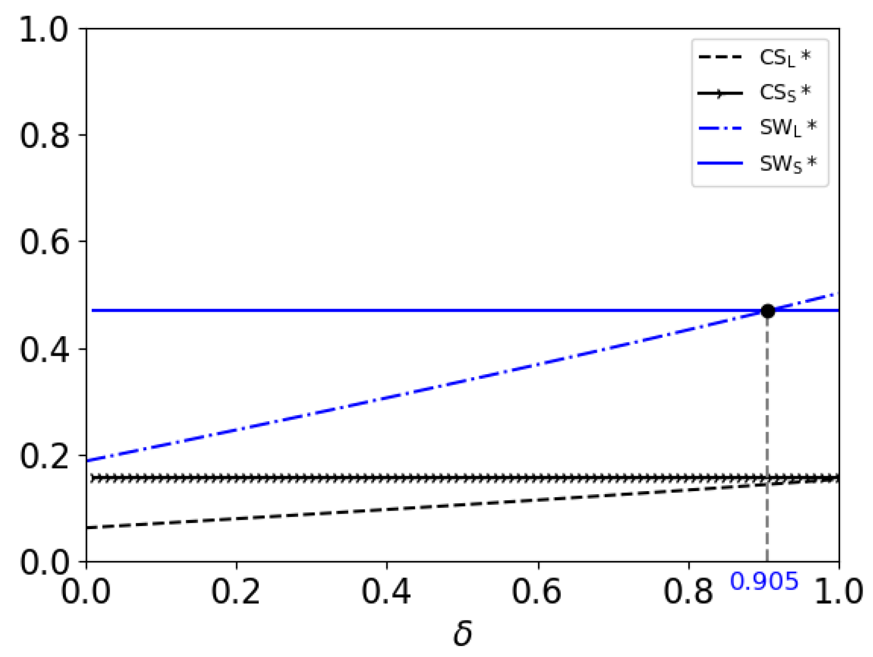
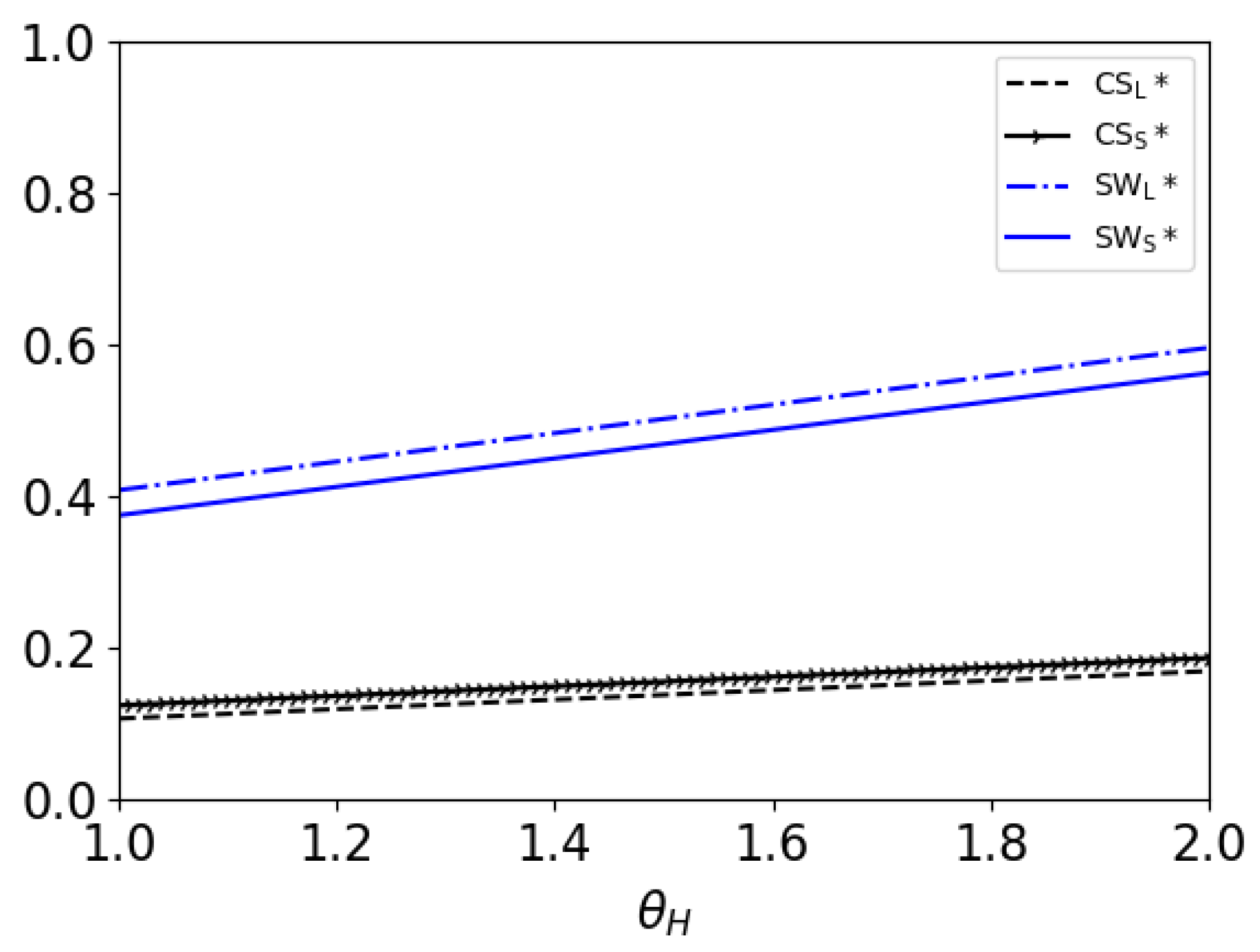
Figure 2 shows that the consumer surplus and the social welfare both increase with the discount factor in the LR model. This result indicates that consumers and publisher both benefit from a stronger discount factor. Figure 2 also shows that the consumer surplus in the SR model is higher than that in the LR model; the social welfare in the SR model is higher if δ 0.905 ; the social welfare in the LR model is higher if δ 0.905 . From Theorem 3, it can be seen that the price of the e-book in the SR model is lower than that in the first stage of the LR model. The price of the e-book in the second stage of the LR model falls to less than the price of the e-book in the SR model. As in the previous analysis, the publisher can obtain more consumer surplus by adopting skimming pricing for the e-book under the LR model. Thus, the consumer cannot obtain more surplus in the LR model. This result indicates that most consumers prefer the SR model. However, as mentioned above, the publisher prefers to release the audiobook after the e-book if the consumers are patient enough. In this case, the publisher can obtain more profit, which results in a higher social welfare.

5.2. Effects of Percentage of High-Value Consumers

In this section, given the values of δ and θ H , as δ = 0.1 , 0.5 , 1 and θ H = 1.5 , we explore the effects of the high-value consumers percentage λ on the consumer surplus and the social welfare.
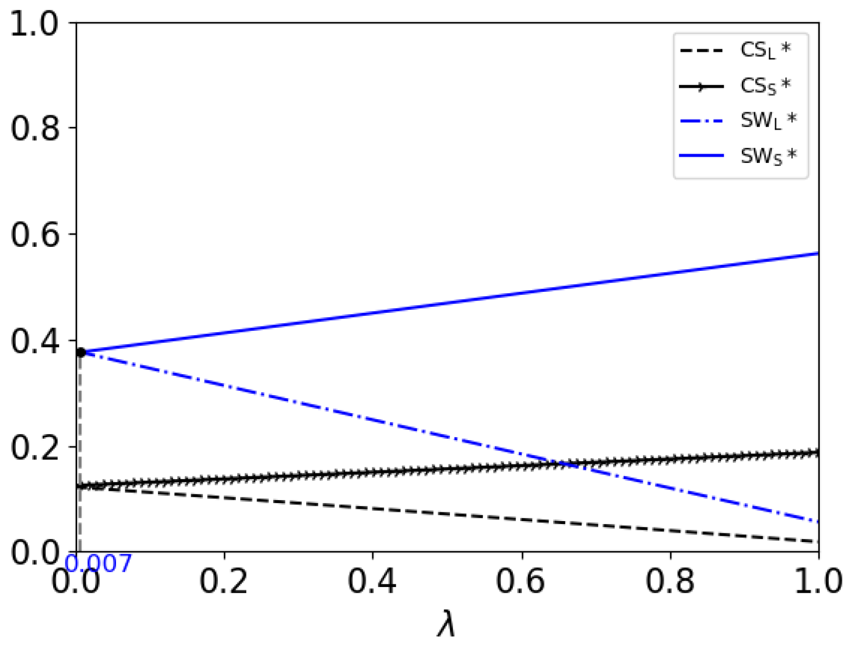
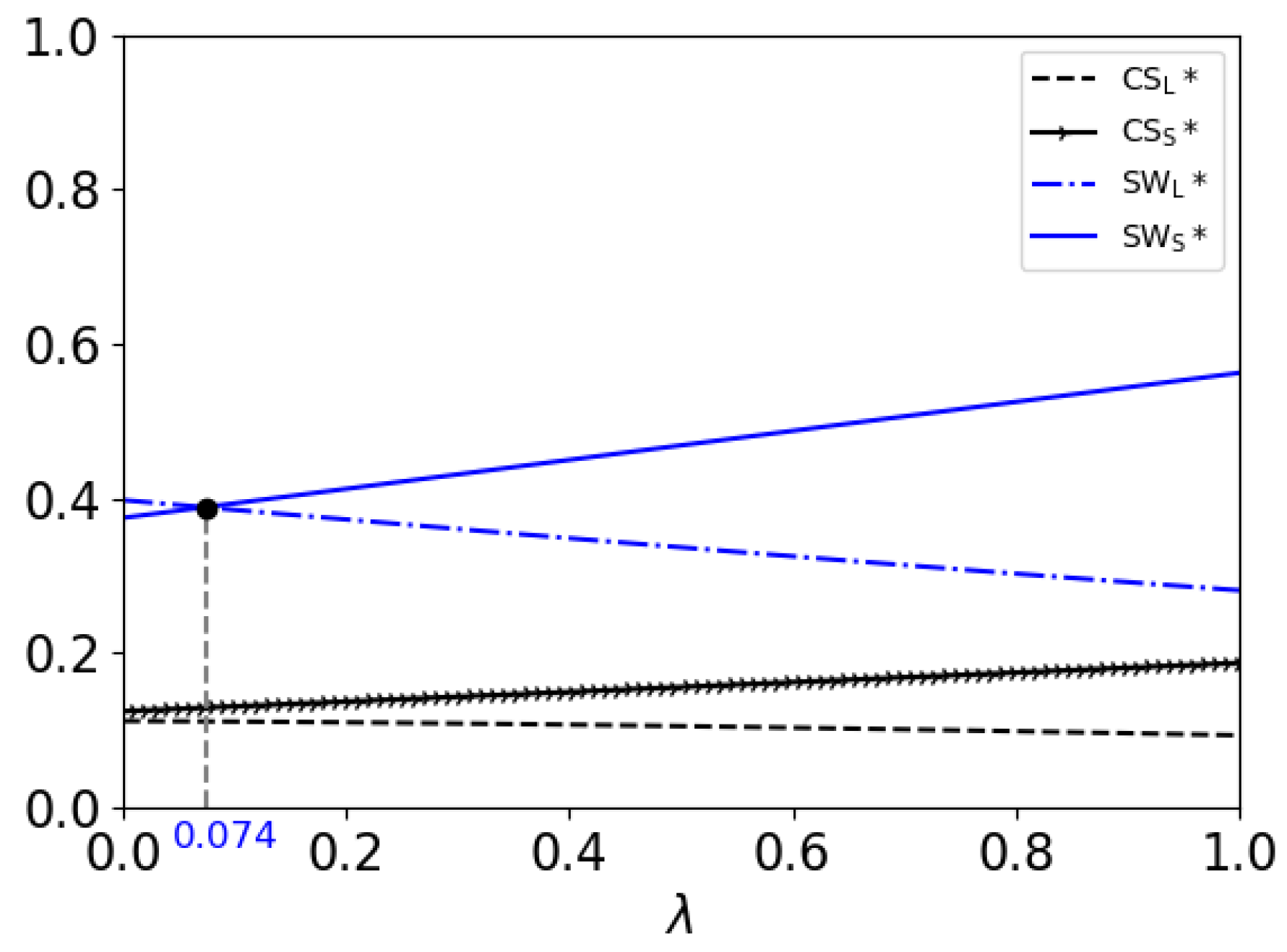
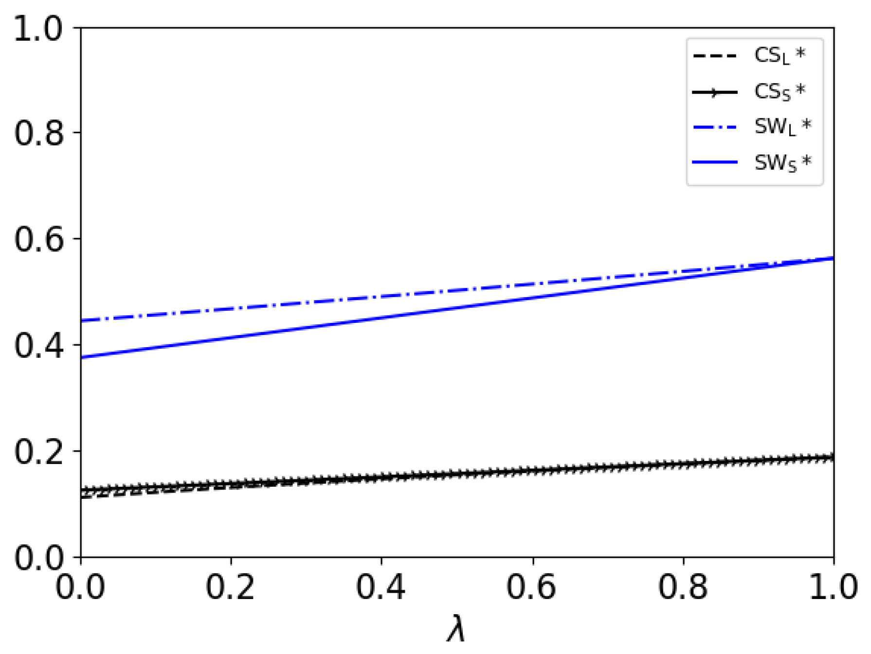
Figure 3, Figure 4 and Figure 5 show the results.
1.
The consumer surplus in the SR model is higher than that in the LR model. This result is the same as that in Section 5.1.
2.
When δ = 0.1 , 0.5 , C S L and S W L both decrease with λ ; when δ = 1 , C S L and S W L both increase with λ . In addition, C S S and S W S both increase with λ .
This result shows that in the LR model, as the percentage of high-value consumers increases, the consumer surplus and the social welfare will both decrease if the consumers’ patience is not strong enough; but if the consumers have enough patience, both the firm and consumers can benefit. In the SR model, the firm and consumers can both benefit from a higher percentage of high-value consumers.
3.
When δ = 0.1 , the social welfare in the SR model is higher than that in the LR model if λ 0.007 ; otherwise, if λ 0.007 , the social welfare in the LR model is higher. When δ = 0.5 , the social welfare in the SR model is higher than that in the LR model if λ 0.074 ; otherwise, if λ 0.074 , the social welfare in the LR model is higher. When δ = 1 , the social welfare in the LR model is higher than that in the SR model.
From Figure 2, we can see that in the LR model, the patience of the consumers helps to improve the social welfare. But, the percentage of high-value consumers hurts the social welfare when the patience of the consumers is not strong enough. Thus, as the patience of the consumers increases, the condition for the percentage of high-value consumers, under which the social welfare is higher in the LR model, will be less strict.

5.3. Effects of High-Value Consumers’ Acceptance Level of Audiobook

In this section, given the values of δ and λ , as δ = 0.1 , 0.5 , 1 and λ = 0.5 , we explore the effects of the high-value consumers’ acceptance level of the audiobook θ H on the consumer surplus and the social welfare.
In Figure 6, subscripts 1, 2, and 3 correspond to δ = 0.1 , 0.5 , and 1, respectively. From Figure 6, we can see that:
1.
π L and π S both increase with θ H . As the above analysis shows, a higher acceptance level results in a higher price of the audiobook, thus the publisher can obtain more profit from the audiobook. Therefore, he can obtain more total profits.
2.
When δ = 0.1 , 0.5 , π L π S ; when δ = 1 , π L π S . From the above analysis, it can be seen that a stronger patience of the consumers helps the monopolist to choose the LR model. When the consumers are less patient, the monopolist prefers the SR model. But when the patience of the consumers is strong enough, the monopolist prefers the LR model. This result agrees with Theorem 3.
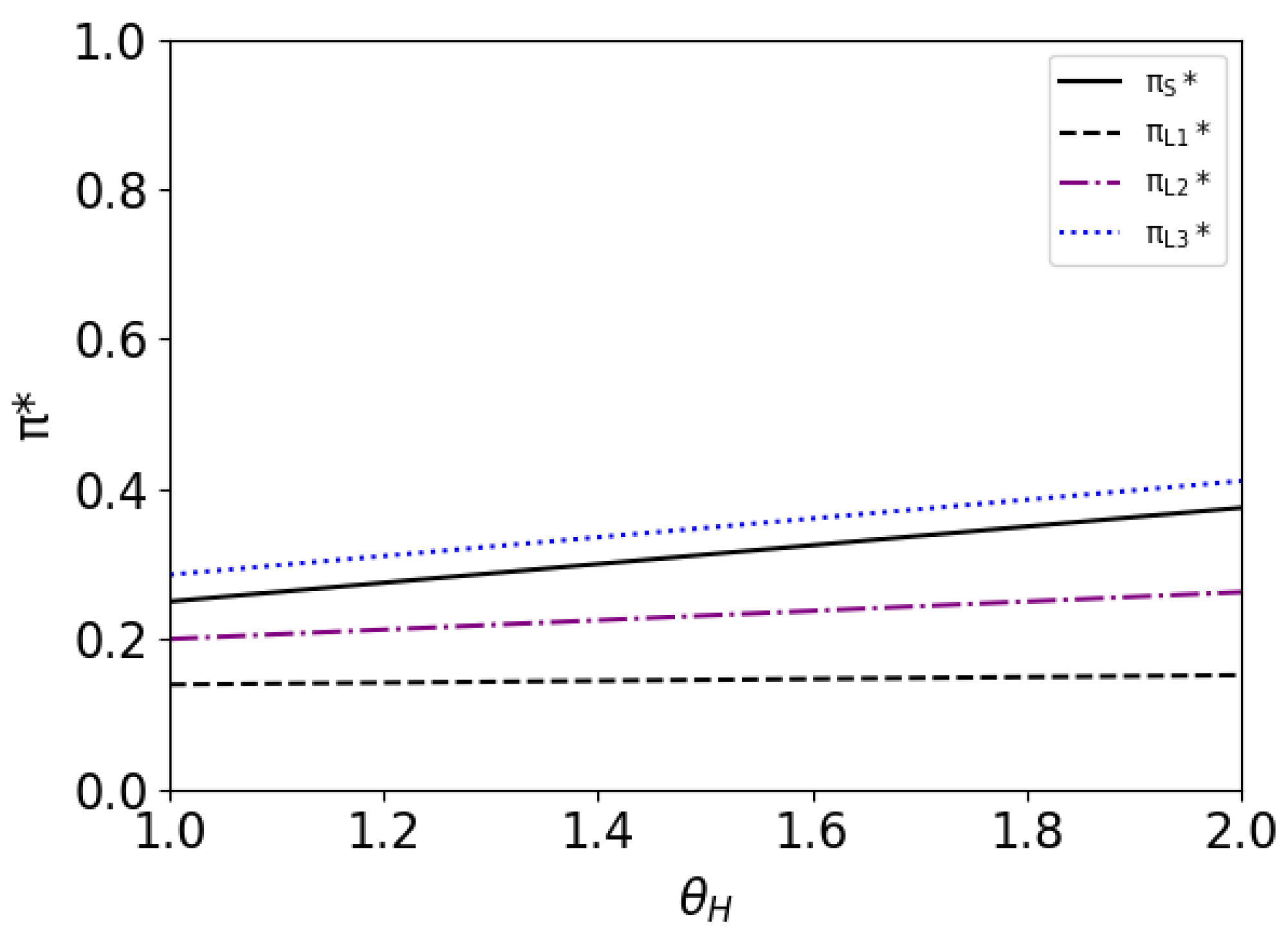
Figure 6. Publisher’s profit relations with high-value consumers’ acceptance level for audiobook in two models when δ = 0.1 , 0.5 , 1 .
Systems 12 00033 g006
Figure 7, Figure 8 and Figure 9 show the following results:
1.
The consumer surplus in the SR model is higher than that in the LR model. This result is the same as those in Section 5.1 and Section 5.2. This means that no matter how these three factors ( δ , λ , θ H ) change, this result always holds.
2.
C S L and S W L , C S S and S W S all increase with θ H .
This result shows that as the acceptance level of high-value consumers increases, the consumers can obtain more surplus. Further, as shown in Theorem 2, the publisher’s profit will also rise with the acceptance level. Thus, a higher acceptance level will result in higher social welfare.
3.
When δ = 0.1 , 0.5 , the social welfare in the SR model is higher than that in the LR model; when δ = 1 , the social welfare in the LR model is higher than that in the SR model.
From Figure 6, it can be seen that when δ = 0.1 , 0.5 , π L π S ; when δ = 1 , π L π S . Further, from Figure 7, it can be seen that C S L C S S . Thus, this result follows.

6. Discussion

Based on the results obtained from the theoretical analysis in the previous sections and the above numerical simulations, we sum our main results and the relations between the discount factor δ , the high-value consumers percentage λ , and the high-value consumers’ acceptance level for the audiobook θ H with the publisher’s pricing strategies and profits, as well as the consumer surplus and the social welfare, in the following findings.
Based on the main result, Theorem 3, the following finding can be obtained.
Finding 1. 
Releasing the audiobook after the e-book is better for the publisher if consumers have enough patience; but if consumers are less patient, it is better for the publisher to release the audiobook and the e-book simultaneously.
Generally, consumers do not have enough patience with new books. Most readers expect to be able to purchase the new book as soon as possible, no matter which version the publisher releases. On the contrary, consumers may be more patient with classic books. Our finding suggests that releasing the e-book and audible versions simultaneously may be better for some new books, but releasing the audible version after the e-book version may be more suitable for some classic books. This finding may help explain the following realities of Amazon publishing.
On Amazon.com, we can find that most recently published books’ various versions are simultaneously released. For example, for «A Promised Land», written by Barack Obama, as the top of the list (until 26 November 2020) among New Releases in Audible Books & Originals on Amazon.com, its Kindle and audible editions were simultaneously released on 17 November 2020. For «Ready Player Two: A Novel», written by Ernest Cline, the second-ranked of the list, its Kindle and audible editions were simultaneously released on 24 November 2020. For «Greenlights», written by Matthew McConaughey, third place in the list, its Kindle and audible editions were simultaneously released on 20 October 2020. For other books in the top ten of the list, such as «Becoming», «Rhythm of War: The Stormlight Archive, Book 4», «The Awakening: The Dragon Heart Legacy, Book 1», and «Daylight (An Atlee Pine Thriller Book 3)», their Kindle and audible editions were all simultaneously released. From Amazon.com, we can also see that the classic novel «Don Quixote»’s Kindle edition was released on 29 January 2009, then its audible book was released on 29 October 2012; For the French children’s book «The Little Prince», its Kindle edition was first released on 19 May 2018, then its audible version was released on 23 May 2020.
By comparing the optimal prices in Theorem 3, the following conclusion can be easily obtained.
Finding 2. 
Whether or not the publisher releases the audiobook after the e-book, the price of the audiobook is higher than the price of the e-book when these two kinds of books are sold in the market simultaneously; if the publisher releases the audiobook after the e-book, he should adopt a skimming pricing strategy for the e-book.
This finding suggests that the publisher should set a higher price for the audiobook than the e-book. In addition, the publisher should lower the price of the e-book when the audiobook is released to the market. The intuition behind this result is obvious. In the first stage, the publisher can obtain more profit by setting a higher price for the e-book since there is only the e-book to be sold in the market. By the second stage, with the consumers’ valuation falling and the competition from the audiobook, lowering the price of the e-book may be a better choice for the publisher.
Notably, the cost of audiobooks is intrinsically higher than that of e-books, which could be one reason of leading to the fact that the audiobook is more expensive than the e-book. Ref. [38] has a similar analysis. However, the costs of digital products are sunk. This cost does not change the optimal strategy in our model. Thus, from another angle, Finding 2 helps to explain the fact that almost all books’ audible versions are much more expensive than their e-book versions on Amazon Audible when the independently priced Kindle edition and audiobook of a particular book are sold at the same time. Finding 2 also helps to explain why the price of a book’s Kindle edition goes down when its audible edition is released.
We can find the following book examples to support the above realities, in addition to Figure 1 in the Introduction. See Figure 10 as an example, on 17 November 2020, when Amazon released the Kindle and audible editions of the book «A Promised Land», written by Barack Obama, simultaneously. From Figure 10, it can be seen that the Kindle edition was priced at USD 17.99, whereas the audible edition was USD 39.81.
From Figure 11 and Figure 12, we can see that: when Amazon first released the Kindle edition of the French children’s book «The Little Prince» on 19 May 2018, it was priced at USD 0.99. When its audible version was released on 23 May 2020, the audible edition was priced at USD 17.95, whereas the price of the Kindle edition dropped to USD 0.2.
From Theorem 2, we can investigate how the factors δ , λ , and θ H affect the publisher’s optimal strategy in the LR model. The corresponding conclusions can be summarized as the following Findings 3–5.
First, the first-order derivatives of p e 1 * , p e 2 * , p a * , D e 1 * , D e 2 * , D e * , D a * , and π * with respect to δ are:
d p e 1 * d δ = 2 ( 1 + δ ) 4 δ ( 1 λ ) 2 0 , d p e 2 * d δ = 4 ( 1 + δ ) 4 δ ( 1 λ ) 2 0 , d p a * d δ = 2 ( 1 + δ ) θ H 4 δ ( 1 λ ) + δ ( 1 λ ) θ H ( 4 δ ( 1 λ ) ) ( 1 λ ) ( 2 δ ) 2 4 δ ( 1 λ ) 2 0 , d D e 1 * d δ = 2 ( 1 λ 2 ) 4 δ ( 1 λ ) 2 0 , d D e 2 * d δ = 1 λ 2 4 δ ( 1 λ ) 2 0 , d D e * d δ = 1 λ 2 4 δ ( 1 λ ) 2 0 , d D a * d δ = 0 , d π * d δ = 2 λ ( 2 δ ( 1 λ ) ) θ H + δ ( 1 λ ) ( 4 δ ( 1 λ ) ) + ( 1 λ ) δ λ θ H ( 4 δ ( 1 λ ) ) + δ ( 1 λ ) + 4 ( 1 λ ) 4 4 δ ( 1 λ ) 2 0 .
To sum up, we have the following conclusion.
Finding 3. 
If the publisher releases the audiobook after the e-book, as the discount factor increases, the price of the e-book in the two stages and the price of the audiobook will all rise, the publisher’s profit, the consumer surplus, and the social welfare will all increase.
A higher discount factor δ means that consumers have more patience for the e-book. The above conclusion suggests that the publisher should set a higher price for his e-book and audiobook if consumers are more patient. The underlying reason behind this is that if consumers are more patient, there will be more consumers to enter the second stage. In the second stage, the consumers’ valuations for the e-book and the audiobook will not fall quickly. The publisher could set a higher prices for the e-book and the audiobook to reap more profits. In the first stage, there is no need for the publisher to adopt a low-price strategy to keep low-value consumers. On the contrary, if he sets a higher price for the e-book in the first stage, it will drive more consumers into the second stage, thereby promoting sales of the e-book in the second stage. Even if the publisher has to bear a profit loss of the e-book in the first stage, he can still gain enough profit from the the e-book and the audiobook in the second stage to make up for the profit loss in the first-stage. Thus, the publisher can benefit from a higher discount factor. If consumers are more patient, their valuations for the books will not fall markedly. Even though the prices of the books are higher, the consumers still can obtain more surpluses. Likewise, the publisher could obtain more profit by setting a higher price for his products when consumers are more patient. Thus, a stronger discount factor will also improve the social welfare.
Second, based on Theorem 2, taking the first-order derivatives of p e 1 * , p e 2 * , p a * , D e 1 * , D e 2 * , D e * , D a * , and π * with respect to λ , we have:
d p e 1 * d λ = δ ( 2 δ ) 4 δ ( 1 λ ) 2 0 , d p e 2 * d λ = 2 δ ( 2 δ ) 4 δ ( 1 λ ) 2 0 , d p a * d λ = 2 δ ( 2 δ ) 4 δ ( 1 λ ) 2 0 , d D e 1 * d λ = 4 δ ( 2 δ ) 4 δ ( 1 λ ) 2 0 , d D e 2 * d λ = δ 2 ( 1 λ ) 2 4 ( 2 δ + 2 δ λ ) 2 4 δ ( 1 λ ) 2 0 , d D e * d λ = d D e 1 * d λ + d D e 2 * d λ 0 , d D a * d λ = 1 2 0 , d π * d λ = ( θ H 1 ) δ 3 λ 2 + 2 ( θ H 1 ) δ 2 ( 4 δ ) λ ( 4 δ ) 4 + ( θ H 1 ) δ 2 4 δ θ H 4 δ 4 4 δ ( 1 λ ) 2 = ( θ H 1 ) δ 3 ( λ λ 1 ) ( λ λ 2 ) 4 4 δ ( 1 λ ) 2 ,
where λ 1 , 2 = ( θ H 1 ) δ 2 ( 4 δ ) ± 2 δ ( 2 δ ) δ ( θ H 1 ) ( θ H 1 ) δ 3 . Further, by computation, there are λ 1 1 if θ H 4 + δ 2 4 δ ; 0 λ 1 1 if 4 + δ 2 4 δ θ H δ 3 4 δ 2 + 16 δ ( 4 δ ) 2 ; λ 1 0 if θ H δ 3 4 δ 2 + 16 δ ( 4 δ ) 2 ; λ 2 0 . Then, the publisher’s profit π * is increasing function of the high-value consumers percentage λ if θ H δ 3 4 δ 2 + 16 δ ( 4 δ ) 2 , or, 4 + δ 2 4 δ θ H δ 3 4 δ 2 + 16 δ ( 4 δ ) 2 and λ λ 1 ; π * is a decreasing function of the high-value consumers percentage λ if 4 + δ 2 4 δ θ H δ 3 4 δ 2 + 16 δ ( 4 δ ) 2 and λ λ 1 , or θ H 4 + δ 2 4 δ .
To sum up, we have the following conclusion.
Finding 4. 
If the publisher releases the audiobook after the e-book, as the percentage of high-value consumers increases, the price of the e-book in the two stages and the price of the audiobook will all rise; the publisher’s profit, the consumer surplus, and the social welfare will increase if the consumers have enough patience, otherwise they will decrease.
The above conclusion suggests that the publisher should set a higher price for his e-book and audiobook if there are increasing high-value consumers. The reason behind this result may be that when there are more high-value consumers, the demand for the audiobook will rise even though the price of the audiobook is higher. In this case, the sales of the audiobook is the main profit source for the publisher. It is unwise for the publisher to adopt a low-price strategy for keeping low-value consumers.
This conclusion also suggests that the publisher should strive to turn low-value consumers into high-value consumers when high-value consumers’ acceptance level for the audiobook is higher than a certain level; otherwise, the publisher should retain low-value consumers when high-value consumers’ acceptance level for the audiobook is relatively low. The underlying reason may be that when high-value consumers’ acceptance level for the audiobook is relatively high, the publisher can achieve more profit from the audiobook, which can make up for the profit loss of the e-book. However, when high-value consumers’ acceptance level for the audiobook is relatively low, the publisher cannot achieve enough profit from the audiobook to make up for the profit loss of the e-book. Thus, in this time, the publisher’s total profit will fall as the percentage of high-value consumers rises.
Finally, from Theorem 3 and the above numerical analysis, the following conclusion can be easily obtained.
Finding 5. 
Whether or not the publisher releases the audiobook after the e-book, as the high-value consumers’ acceptance level for the audiobook increases, the price of the e-book is not affected, but the price of the audiobook will rise; the publisher’s profit, the consumer surplus, and the social welfare will also increase with the acceptance level.
The above conclusion suggests that the publisher should set a higher price for his audiobook if high-value consumers’ acceptance level for the audiobook is higher. The prices and demand for the e-book in the two stages will not be affected by this acceptance level. This means that the publisher’s profit from the e-book will not be affected by this acceptance level, but the publisher can obtain more profit from the audiobook. Thus, in total, the publisher can still benefit from a higher acceptance level of high-value consumers’ for the audiobook.
This result also indicates that the consumers and the publisher will both benefit from high-quality audiobooks. The higher the quality of the audiobook, the greater the consumers’ acceptance level of the audiobook. This result suggests that the publisher should devote efforts to improving the quality of the audiobook from various aspects, thereby enhancing the consumers’ acceptance level of the audiobook, especially turning more low-value consumers into high-value consumers. Now, with worldwide demand for audiobooks soaring, the stars want to be heard reading unabridged books. For example, Audible is the largest producer of audiobooks in the world. It signed some talented performers like Emma Thompson, Mahershala Ali, and Nick Offerman to interpret great texts through nuanced performances. These efforts mean millions of listeners can enjoy audiobooks anytime, anywhere, and bring wonderful experiences to consumers, which in turn greatly promotes the sales of audiobooks.

7. Conclusions

In this paper, we analyze the optimal pricing strategies of a monopolistic publisher under two different release models: releasing a book with audible version and e-book version simultaneously and releasing a book in its audible version after its e-book version. By comparing the profits in the two models, we give the conditions under which the publisher should release the audiobook after the e-book. Our results show that if consumers have enough patience, the publisher should release the audiobook after the e-book, and he should adopt a skimming pricing strategy for the e-book in this release model. Otherwise, if consumers are less patient, the publisher should release the audiobook and the e-book simultaneously. Further, our results indicate that whether or not the publisher releases the audiobook after the e-book, he should set a higher price for the audiobook than e-book. This helps to explain why the price of audiobooks is higher than that of e-books in the real market. Our study could provide references for researchers in related fields, and also provides some valuable explorations for managerial practitioners to make decisions on pricing and release strategies.
We propose several possible future research directions and suggestions. First, we focus on a comparative analysis of the two release models: releasing the audiobook and e-book simultaneously and releasing the audiobook after the e-book. However, we do not consider the case under which the e-book is released after the audiobook. It would be more complex to analyze and compare three models. Based on this study, we will explore this issue in our future research. Second, we consider a monopolistic publisher who both manufactures and sells the books to consumers in this study. In reality, some manufacturers are not usually retailers. Considering manufacturers and retailers as separate players in the model would be a meaningful study. In addition, we focus on the case of monopolist in this study. It would be interesting to investigate how would the optimal choice of the publisher changes if multiple publishers are competing against each other in this model. Last but not least, we only perform a preliminary extension to this study by involving printed books in the model, and basing the models on some rigorous assumptions. It would be more complicated and also be meaningful to conduct research by incorporating printed books in the model, both analytically and empirically. We are fully aware that the results in this study are only suggestive. Although we have tried to make the assumptions made in the model as reasonable as possible, they still need to be justified by a substantial empirical endeavor. We hope that this paper can serve as a stepping stone for future empirical work.

Funding

This research was funded in part by MOE (Ministry of Education in China) Project of Humanities and Social Sciences [grant number 22YJC630203], and the Social Science Foundation of Hubei Province of China [grant number HBSKJJ20233291].

Data Availability Statement

The data that support the findings of this study are available from the corresponding author upon reasonable request.

Conflicts of Interest

The authors declare no conflicts of interest.

Appendix A. Derivation of Demand for the E-Book and the Audiobook under the SR Model
By analysis, we have the following conclusions:
(1) If p a θ H p e , then there is v ¯ H p a θ H p e , v ¯ L 0 p a θ L p e . We have the following results:
High-value consumers in the interval [ v ¯ H , 1 ] will buy the audiobook and high-value consumers in the interval [ p e , v ¯ H ] will buy the e-book; other high-value consumers choose not to buy any product. Low-value consumers in the interval [ p e , 1 ] will buy the e-book; other low-value consumers choose not to buy any product. This may be because the price of the audiobook is so high that no low-value consumers will buy the audiobook.
(2) If θ L p e p a θ H p e , then we have v ¯ H p a θ H p e p a θ L , v ¯ L p e p a θ L .
High-value consumers in the interval [ p a θ H , 1 ] will buy the audiobook; other high-value consumers choose not to buy any product. This may be because the price of the e-book is too high for the high-value consumers, no one will buy the e-book. Low-value consumers in the interval [ p e , 1 ] will buy the e-book; other low-value consumers choose not to buy any product.
(3) If p a θ L p e , then there is v ¯ H p a θ H p a θ L p e v ¯ L . We have the following results:
High-value consumers in the interval [ p a θ H , 1 ] will buy the audiobook; other high-value consumers choose not to buy any product. This may be because the price of the audiobook is so low for the high-value consumers that no one will buy the e-book. Low-value consumers in the interval [ p a θ L , v ¯ L ] will buy the audiobook and low-value consumers in the interval [ v ¯ L , 1 ] will buy the e-book; other low-value consumers choose not to buy any product.
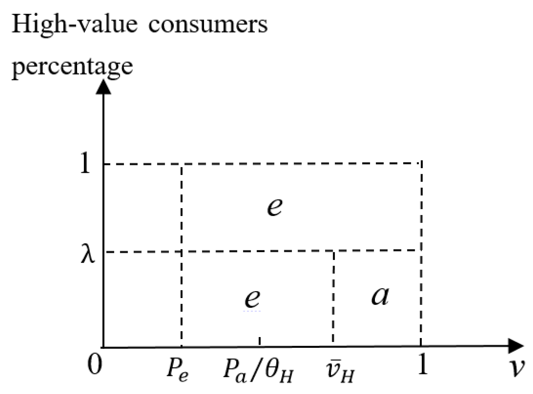
See Figure A1 for an illustration of consumers’ choice when p a θ H p e .
In Figure A1, the area below letter λ along the vertical axis denotes high-value consumers, those with a horizontal interval [ p e , v ¯ H ] buy the e-book (indicated by letter e), and those with a horizontal interval [ v ¯ H , 1 ] buy the audiobook (indicated by letter a). Similarly, among the low-value consumers (above letter λ along the vertical axis in Figure A1), those with a horizontal interval [ p e , 1 ] buy the e-book, and the rest buy nothing. Thus, the areas [ p e , v ¯ H ] × [ 0 , λ ] and [ p e , 1 ] × [ λ , 1 ] correspond to the demand for the e-book, the area [ v ¯ H , 1 ] × [ 0 , λ ] corresponds to the demand for the audiobook.
Figure A1. An illustration of consumers’ choice when p a θ H p e .
Systems 12 00033 g0a1
By similar analysis for the remaining two cases: θ L p e p a θ H p e , p a θ L p e , and computing the corresponding area, we can derive the demand functions of the e-book and the audiobook as follows:
D e = ( 1 λ ) ( 1 p e ) + λ ( p a p e θ H 1 p e ) p a θ H p e ( 1 λ ) ( 1 p e ) θ L p e p a θ H p e ( 1 λ ) ( 1 p e p a 1 θ L ) p a θ L p e
D a = λ ( 1 p a p e θ H 1 ) p a θ H p e λ ( 1 p a θ H ) θ L p e p a θ H p e λ ( 1 p a θ H ) + ( 1 λ ) ( p e p a 1 θ L p a θ L ) p a θ L p e

Appendix B. Derivation of Demand for the E-Book and the Audiobook in the Second Stage under LR Model

According to the previous analysis, there are u e 2 0 and u e 2 u a L if and only if v p e 2 δ and v v ¯ L 2 ; u a L 0 and u a L u e 2 if and only if v p a δ θ L and v v ¯ L 2 ; u e 2 0 and u e 2 u a H if and only if v p e 2 δ and v v ¯ H 2 ; u a H 0 and u a H u e 2 if and only if v p a δ θ H and v v ¯ H 2 . That is, a low-value consumer will buy the e-book if her valuation v m a x p e 2 δ , v ¯ L 2 , and she will buy the audiobook if her valuation v [ p a δ θ L , v ¯ L 2 ] under the condition that p a δ θ L v ¯ L 2 ; a high-value consumer will buy the e-book if her valuation v [ p e 2 δ , v ¯ H 2 ] under the condition that p e 2 δ v ¯ H 2 , and she will buy the audiobook if her valuation v m a x p a δ θ H , v ¯ H 2 .
Further, there are v ¯ L 2 p e 2 δ = θ L p e 2 p a δ ( 1 θ L ) , v ¯ L 2 p a δ θ L = θ L p e 2 p a δ θ L ( 1 θ L ) , v ¯ H 2 p e 2 δ = p a θ H p e 2 δ ( θ H 1 ) , v ¯ H 2 p a δ θ H = p a θ H p e 2 δ θ H ( θ H 1 ) . To analyze the demand for the e-book and the audiobook in the second stage, we divide our analysis into the following four cases.
Remark A1. 
p e 2 δ p e 1
Some of the low-value consumers who do not obtain a positive utility from the e-book in the first stage may achieve a positive utility from the e-book in the second stage under this case. All consumers in this stage are faced with three choices: buying the e-book, buying the audiobook, or doing nothing.
(1) If p a p e 2 + δ ( θ H 1 ) , there are v ¯ H 2 1 , v ¯ L 2 p e 2 δ p a δ θ L .
In this case, this may be because the price of the audiobook is so high that no consumers will buy the audiobook. Low-value consumers in the interval [ p e 2 δ , p e 1 ] and high-value consumers in the interval [ p e 2 δ , 1 ] will buy the e-book; other consumers choose not to buy any product.
(2) If θ H p e 2 p a p e 2 + δ ( θ H 1 ) , there are p e 2 δ p a δ θ H v ¯ H 2 1 , v ¯ L 2 p e 2 δ p a δ θ L .
Low-value consumers in the interval [ p e 2 δ , p e 1 ] will buy the e-book; other low-value consumers choose not to buy any book. This may be because the price of the audiobook is still too high for low-value consumers, no one will buy the audiobook. High-value consumers in the interval [ p e 2 δ , v ¯ H 2 ] will buy the e-book and high-value consumers in the interval [ v ¯ H 2 , 1 ] will buy the audiobook; other high-value consumers choose not to buy any product.
(3) If θ L p e 2 p a θ H p e 2 , there are v ¯ H 2 p a δ θ H p e 2 δ 1 , v ¯ L 2 p e 2 δ p a δ θ L .
Low-value consumers in the interval [ p e 2 δ , p e 1 ] will buy the e-book; other low-value consumers choose not to buy any book. High-value consumers in the interval [ p a δ θ H , 1 ] will buy the audiobook; other high-value consumers choose not to buy any product.
(4) If p e 2 δ ( 1 θ L ) p e 1 p a θ L p e 2 , there are v ¯ H 2 p a δ θ H p e 2 δ 1 , p a δ θ L p e 2 δ v ¯ L 2 p e 1 .
Low-value consumers in the interval [ v ¯ L 2 , p e 1 ] will buy the e-book; and low-value consumers in the interval [ p a δ θ L , v ¯ L 2 ] will buy the audiobook; other low-value consumers choose not to buy any book. High-value consumers in the interval [ p a δ θ H , 1 ] will buy the audiobook; other high-value consumers choose not to buy any product.
(5) If p a p e 2 δ ( 1 θ L ) p e 1 , there are v ¯ H 2 p a δ θ H p a δ θ L p e 2 δ p e 1 v ¯ L 2 .
Low-value consumers in the interval [ p a δ θ L , p e 1 ] and high-value consumers in the interval [ p a δ θ H , 1 ] will buy the audiobook. Other consumers choose not to buy any product. In this case, this may be because the price of the audiobook is so low that no consumers will buy the e-book.
Above all, if p e 2 δ p e 1 , the demand functions of the e-book and the audiobook in the second stage can be concluded as follows:
D e 2 = ( 1 λ ) ( p e 1 p e 2 δ ) + λ ( 1 p e 2 δ ) p a p e 2 + δ ( θ H 1 ) ( 1 λ ) ( p e 1 p e 2 δ ) + λ ( v ¯ H 2 p e 2 δ ) θ H p e 2 p a p e 2 + δ ( θ H 1 ) ( 1 λ ) ( p e 1 p e 2 δ ) θ L p e 2 p a θ H p e 2 ( 1 λ ) ( p e 1 v ¯ L 2 ) p e 2 δ ( 1 θ L ) p e 1 p a θ L p e 2 0 p a p e 2 δ ( 1 θ L ) p e 1
D a = 0 p a p e 2 + δ ( θ H 1 ) λ ( 1 v ¯ H 2 ) θ H p e 2 p a p e 2 + δ ( θ H 1 ) λ ( 1 p a δ θ H ) θ L p e 2 p a θ H p e 2 ( 1 λ ) ( v ¯ L 2 p a δ θ L ) + λ ( 1 p a δ θ H ) p e 2 δ ( 1 θ L ) p e 1 p a θ L p e 2 ( 1 λ ) ( p e 1 p a δ θ L ) + λ ( 1 p a δ θ H ) p a p e 2 δ ( 1 θ L ) p e 1
Remark A2. 
δ p e 1 p e 2 δ
Since p e 2 δ p e 1 under this case, the low-value consumers who do not obtain a positive utility from the e-book in the first stage still cannot obtain a positive utility from the e-book in the second stage. Thus, no low-value consumers will buy the e-book in the second stage. Specifically,
(1) If p a p e 2 + δ ( θ H 1 ) , there are v ¯ H 2 1 , v ¯ L 2 p e 2 δ p a δ θ L , p e 2 δ p a δ θ H v ¯ H 2 . High-value consumers in the interval [ p e 2 δ , 1 ] will buy the e-book. Other consumers choose not to buy any product.
(2) If θ H p e 2 p a p e 2 + δ ( θ H 1 ) , there are p e 2 δ p a δ θ H v ¯ H 2 1 , v ¯ L 2 p e 2 δ p a δ θ L . High-value consumers in the interval [ p e 2 δ , v ¯ H 2 ] will buy the e-book; and high-value consumers in the interval [ v ¯ H 2 , 1 ] will buy the audiobook. Other consumers choose not to buy any product.
(3) If θ L p e 2 p a θ H p e 2 , there are v ¯ H 2 p a δ θ H p e 2 δ 1 , v ¯ L 2 p e 2 δ p a δ θ L . High-value consumers in the interval [ p a δ θ H , 1 ] will buy the audiobook. Other consumers choose not to buy any product.
(4) If δ θ L p e 1 p a θ L p e 2 , there are v ¯ H 2 p a δ θ H p e 2 δ 1 , p e 1 p a δ θ L p e 2 δ v ¯ L 2 . High-value consumers in the interval [ p a δ θ H , 1 ] will buy the audiobook. Other consumers choose not to buy any product.
(5) If p a δ θ L p e 1 , there are v ¯ H 2 p a δ θ H p e 2 δ 1 , p a δ θ L p e 1 p e 2 δ v ¯ L 2 . Low-value consumers in the interval [ p a δ θ L , p e 1 ] and high-value consumers in the interval [ p a δ θ H , 1 ] will buy the audiobook. Other consumers choose not to buy any product.
Above all, if δ p e 1 p e 2 δ , the demand functions of the e-book and the audiobook in the second stage can be concluded as follows:
D e 2 = λ ( 1 p e 2 δ ) p a p e 2 + δ ( θ H 1 ) λ ( v ¯ H 2 p e 2 δ ) θ H p e 2 p a p e 2 + δ ( θ H 1 ) 0 p a θ H p e 2
D a = 0 p a p e 2 + δ ( θ H 1 ) λ ( 1 v ¯ H 2 ) θ H p e 2 p a p e 2 + δ ( θ H 1 ) λ ( 1 p a δ θ H ) δ θ L p e 1 p a θ H p e 2 ( 1 λ ) ( p e 1 p a δ θ L ) + λ ( 1 p a δ θ H ) p a δ θ L p e 1
Remark A3. 
δ p e 2 θ H θ L δ
No consumers can obtain a positive utility from the e-book under this case since p e 2 δ 1 p e 1 . Thus, no consumers will buy the e-book in the second stage. That is, the demand for the e-book is 0 in the second stage. Next, we analyze the demand for the audiobook. Specifically,
(1) If p a δ θ H , there are 1 p a δ θ H p a δ θ L . In this case, this may be because the price of the audiobook is so high that no consumers can obtain a positive utility from the audiobook. Thus, no consumers choose to buy any product under this case.
(2) If δ θ L p e 1 p a δ θ H , there are v ¯ H 2 p a δ θ H 1 , p e 1 p a δ θ L . High-value consumers in the interval [ p a δ θ H , 1 ] will buy the audiobook. Other consumers choose not to buy any product.
(3) If p a δ θ L p e 1 , there are v ¯ H 2 p a δ θ H p a δ θ L p e 1 1 p e 2 δ v ¯ L 2 . Low-value consumers in the interval [ p a δ θ L , p e 1 ] and high-value consumers in the interval [ p a δ θ H , 1 ] will buy the audiobook. Other consumers choose not to buy any product.
Above all, if δ p e 2 θ H θ L δ , the demand functions of the e-book and the audiobook in the second stage can be concluded as follows: D e 2 = 0 ,
D a = 0 p a δ θ H λ ( 1 p a δ θ H ) δ θ L p e 1 p a δ θ H ( 1 λ ) ( p e 1 p a δ θ L ) + λ ( 1 p a δ θ H ) p a δ θ L p e 1
Remark A4. 
p e 2 θ H θ L δ
Similarly, no consumers can obtain a positive utility from the e-book under this case since p e 2 δ 1 p e 1 . Thus, the demand for the e-book is 0 in the second stage. Next, we analyze the demand for the audiobook. Specifically,
(1) If p a δ θ H , there is 1 p a δ θ H p a δ θ L . In this case, no consumers can obtain a positive utility from the audiobook. Thus, all consumers choose not to buy any product under this case.
(2) If p a δ θ H , there is v ¯ H 2 p a δ θ H 1 p a δ θ L . High-value consumers in the interval [ p a δ θ H , 1 ] will buy the audiobook. Other consumers choose not to buy any product.
Above all, if p e 2 θ H θ L δ , the demand functions of the e-book and the audiobook in the second stage can be concluded as follows: D e 2 = 0 ,
D a = 0 p a δ θ H λ ( 1 p a δ θ H ) p a δ θ H

Appendix C

Proof of Theorem 1. 
The publisher’s optimization problem is
max p e , p a ( 0 , 1 ) π = p e D e + p a D a ,
where D e , D a are given in Section 3.2.
(1) When p a θ H p e , there is π = p e ( 1 λ ) ( 1 p e ) + λ ( p a p e θ H 1 p e ) + p a λ ( 1 p a p e θ H 1 ) . We first solve for p e * from π p e = 0 , then we substitute it into π p a = 0 and solve for p a * . We obtain p e * = 1 2 , p a * = θ H 2 . To verify the second-order conditions, we derive the 2 × 2 Hessian matrix H. We find H 11 = 2 π p e 2 = 2 ( λ + θ H 1 ) θ H 1 < 0 , and H = 4 λ θ H 1 > 0 . Therefore, π ( p e , p a ) is jointly concave, and its value is maximized at ( p e * , p a * ) . We substitute ( p e * , p a * ) into the demand functions of the e-book and the audiobook D e , D a , and the profit function of the publisher π , then we can obtain the corresponding demands D e = 1 λ 2 , D a = λ 2 , and the publisher’s optimal profit under this case as follows: π 1 = 1 + λ ( θ H 1 ) 4 .
(2) When θ L p e p a θ H p e , there is π = p e ( 1 λ ) ( 1 p e ) + p a λ ( 1 p a θ H ) . Similarly, we first solve for p e * from π p e = 0 , then we substitute it into π p a = 0 and solve for p a * . We can obtain: p e * = 1 2 , p a * = θ H 2 . The following analysis is same as that of the first case. Thus, the publisher’s optimal profit under this case is as follows: π 2 = 1 + λ ( θ H 1 ) 4 .
(3) When p a θ L p e , there is π = p e ( 1 λ ) ( 1 p e p a 1 θ L ) + p a λ ( 1 p a θ H ) + ( 1 λ ) ( p e p a 1 θ L p a θ L ) . We first solve for p e * from π p e = 0 , then we substitute it into π p a = 0 and solve for p a * . We can obtain p e * = 1 θ L 2 + θ L θ H 2 ( ( 1 λ ) θ H + λ θ L ) , p a * = θ L θ H 2 ( ( 1 λ ) θ H + λ θ L ) . Since p a * θ L p e * = ( 1 θ L ) λ θ L ( θ H θ L ) 2 ( ( 1 λ ) θ H + λ θ L ) 0 , then the above solution ( p e * , p a * ) is beyond the constraint condition p a θ L p e . Thus, the optimal solution should be achieved at the boundary condition p a = θ L p e .
We substitute p a = θ L p e into the profit function π and take its first-order derivative with respect to p e . We can obtain p e * = θ H ( 1 λ + λ θ L ) 2 ( ( 1 λ ) θ H + λ θ L 2 ) , p a * = θ L p e * = θ L θ H ( 1 λ + λ θ L ) 2 ( ( 1 λ ) θ H + λ θ L 2 ) . We substitute ( p e * , p a * ) into the demand functions of the e-book and the audiobook D e , D a , and the publisher’s profit function π , then we can obtain: D e = ( 1 λ ) θ H ( 1 λ ) + λ θ L ( 2 θ L θ H ) 2 ( ( 1 λ ) θ H + λ θ L 2 ) , D a = λ ( 2 θ H θ L ) ( 1 λ ) + λ θ L 2 2 ( ( 1 λ ) θ H + λ θ L 2 ) , and the publisher’s optimal profit under this case as follows: π 3 = θ H ( 1 λ + λ θ L ) 2 4 ( ( 1 λ ) θ H + λ θ L 2 ) .
By comparing the above three profits, we have: π 1 = π 2 , π 3 π 1 = λ ( 1 λ ) ( θ H θ L ) 2 4 ( ( 1 λ ) θ H + λ θ L 2 ) 0 , Thus, the optimal profit of the publisher is π 1 . The result follows. □

Appendix D

Proof of Lemma 1. 
When p e 2 δ p e 1 , the publisher’s profit function is π = p e 1 D e 1 + p e 2 D e 2 + P a D a , where D e 1 = ( 1 λ ) ( 1 p e 1 ) , D e 2 , and D a are given in case 2 of Section 3.3
(1) If p a p e 2 + δ ( θ H 1 ) , there is π = ( 1 λ ) p e 1 ( 1 p e 1 ) + p e 2 ( 1 λ ) ( p e 1 p e 2 δ ) + λ ( 1 p e 2 δ ) . Taking the first-order derivative of π with respect to p e 2 and setting the derivation to zero, we have p e 2 = δ ( λ + ( 1 λ ) p e 1 ) 2 . Substituting p e 2 into π , then taking the first-order derivative of π with respect to p e 1 and setting the derivation to zero, we have p e 1 * = 2 + δ λ 4 δ ( 1 λ ) . Substituting the value of p e 1 * back into the previous p e 2 , we have p e 2 * = δ ( 1 + λ ) 4 δ ( 1 λ ) . Since δ ( 1 + λ ) 4 δ ( 1 λ ) δ ( 2 + δ λ ) 4 δ ( 1 λ ) , that is, the above p e 1 * and p e 2 * satisfy the constraint p e 2 δ p e 1 , the maximum value of π can be achieved in this case. Substituting the value combination ( p e 1 * , p e 2 * ) into the profit function π , we can obtain the optimal profit under this case as follows: π 1 = 1 λ + δ λ 4 δ ( 1 λ ) .
(2) If θ H p e 2 p a p e 2 + δ ( θ H 1 ) , there is π = ( 1 λ ) p e 1 ( 1 p e 1 ) + p e 2 ( 1 λ ) ( p e 1 p e 2 δ ) + λ ( v ¯ H 2 p e 2 δ ) + λ p a ( 1 v ¯ H 2 ) . We first solve for p e 2 from π p e 2 = 0 , then we substitute it into π p a = 0 and solve for p a . We can obtain p e 2 = δ ( λ + ( 1 λ ) p e 1 ) 2 , p a = δ ( λ + θ H 1 + ( 1 λ ) p e 1 ) 2 . Substituting the above ( p e 2 , p a ) into π , then taking the first-order derivative of π with respect to p e 1 and setting the derivation to zero, we have p e 1 * = 2 + δ λ 4 δ ( 1 λ ) . Substituting p e 1 * back into the previous p e 2 and p a , we have p e 2 * = δ ( 1 + λ ) 4 δ ( 1 λ ) , p a * = δ θ H ( 4 δ ( 1 λ ) ) ( 1 λ ) ( 2 δ ) 2 ( 4 δ ( 1 λ ) ) . It can be easily verified that the above optimal prices p e 1 * , p e 2 * , p a * satisfy the constraint conditions p e 2 δ p e 1 and θ H p e 2 p a p e 2 + δ ( θ H 1 ) . Thus, the maximum value of π can be achieved in this case. Substituting the value combination ( p e 1 * , p e 2 * , p a * ) into the profit function π , we can obtain the optimal profit under this case as follows: π 2 = δ λ θ H ( 4 δ ( 1 λ ) ) + δ ( 1 λ ) + 4 ( 1 λ ) 4 ( 4 δ ( 1 λ ) ) .
(3) If θ L p e 2 p a θ H p e 2 , there is π = ( 1 λ ) p e 1 ( 1 p e 1 ) + ( 1 λ ) p e 2 ( p e 1 p e 2 δ ) + λ p a ( 1 p a δ θ H ) . We first solve for p e 2 from π p e 2 = 0 , then we substitute it into π p a = 0 and solve for p a . We can obtain p e 2 = δ p e 1 2 , p a = δ θ H 2 . In this case, since δ θ H 2 θ H δ p e 1 2 , the above solutions p e 2 and p a are beyond the constraint p a θ H p e 2 . Thus, the optimal solutions should be on the boundary p a = θ H p e 2 .
Substituting p a = θ H p e 2 into the profit function π , then taking the first-order derivative of π with respect to p e 2 and setting the derivative to zero, we have p e 2 = δ ( ( 1 λ ) p e 1 + λ θ H ) 2 ( 1 λ + λ θ H ) , then p a = δ θ H ( ( 1 λ ) p e 1 + λ θ H ) 2 ( 1 λ + λ θ H ) .
Substituting the above ( p e 2 , p a ) into π , then taking the first-order derivative of π with respect to p e 1 and setting the derivation to zero, we have p e 1 * = 2 ( 1 λ + λ θ H ) + δ λ θ H 4 ( 1 λ + λ θ H ) δ ( 1 λ ) . Substituting p e 1 * back into the previous p e 2 and p a , we have p e 2 * = δ ( 1 λ + 2 λ θ H ) 4 ( 1 λ + λ θ H ) δ ( 1 λ ) , p a * = δ θ H ( 1 λ + 2 λ θ H ) 4 ( 1 λ + λ θ H ) δ ( 1 λ ) . It can be easily verified that the above optimal prices p e 1 * , p e 2 * , p a * satisfy the constraint conditions p e 2 δ p e 1 and θ L p e 2 p a θ H p e 2 . Thus, the maximum value of π can be achieved in this case. Substituting the value combination ( p e 1 * , p e 2 * , p a * ) into the profit function π , we can obtain the optimal profit under this case as follows: π 3 = ( 1 λ + λ θ H ) ( 1 λ + δ λ θ H ) 4 ( 1 λ + λ θ H ) δ ( 1 λ ) .
(4) If p e 2 δ ( 1 θ L ) p e 1 p a θ L p e 2 , there is π = ( 1 λ ) p e 1 ( 1 p e 1 ) + ( 1 λ ) p e 2 ( p e 1 v ¯ L 2 ) + p a ( 1 λ ) ( v ¯ L 2 p a δ θ L ) + λ ( 1 p a δ θ H ) . We first solve for p e 2 from π p e 2 = 0 , then we substitute it into π p a = 0 and solve for p a . We can obtain p e 2 = δ ( 1 θ L ) p e 1 2 + δ θ H θ L ( λ + ( 1 λ ) p e 1 ) 2 ( λ θ L + ( 1 λ ) θ H ) , p a = δ θ H θ L ( λ + ( 1 λ ) p e 1 ) 2 ( λ θ L + ( 1 λ ) θ H ) . In this time, since p a θ L p e 2 = δ λ θ L ( 1 θ L ) ( θ H θ L p e 1 ) 2 ( λ θ L + ( 1 λ ) θ H ) > 0 , which is beyond the constraint p a θ L p e 2 . Thus, the optimal solutions should be on the boundary p a = θ L p e 2 .
Substituting p a = θ L p e 2 into the profit function π , then taking the first-order derivative of π with respect to p e 2 and setting the derivative to zero, we have p e 2 = δ θ H ( ( 1 λ ) p e 1 + λ θ L ) 2 ( 1 λ ) θ H + λ θ L 2 , then p a = δ θ H θ L ( ( 1 λ ) p e 1 + λ θ L ) 2 ( 1 λ ) θ H + λ θ L 2 .
Substituting the above ( p e 2 , p a ) into π , then taking the first-order derivative of π with respect to p e 1 and setting the derivation to zero, we have p e 1 * = δ λ θ H θ L + 2 ( 1 λ ) θ H + 2 λ θ L 2 ( 4 δ ) ( 1 λ ) θ H + 4 λ θ L 2 . Substituting p e 1 * back into the previous p e 2 and p a , we can obtain p e 2 * and p a * which satisfy the constraint conditions. Similarly, we can obtain the optimal profit under this case as follows: π 4 = λ θ L 2 ( 1 λ + δ λ θ H ) + ( 1 λ ) θ H ( 1 λ + δ λ θ L ) ( 4 δ ) ( 1 λ ) θ H + 4 λ θ L 2 .
(5) If p a p e 2 δ ( 1 θ L ) p e 1 , there is π = ( 1 λ ) p e 1 ( 1 p e 1 ) + p a ( 1 λ ) ( p e 1 p a δ θ L ) + λ ( 1 p a δ θ H ) . Taking the first-order derivative of π with respect to p a and setting the derivation to zero, we have p a = δ θ H θ L ( λ + ( 1 λ ) p e 1 ) 2 ( λ θ L + ( 1 λ ) θ H ) . Substituting p a into π , then taking the first-order derivative of π with respect to p e 1 and setting the derivation to zero, we have p e 1 * = 2 ( λ θ L + ( 1 λ ) θ H ) + δ λ θ H θ L 4 ( λ θ L + ( 1 λ ) θ H ) δ ( 1 λ ) θ H θ L . Substituting the value of p e 1 * back into the profit function π , we can obtain the optimal profit under this case as follows: π 5 = ( 1 λ ) ( λ θ L + ( 1 λ ) θ H ) + δ λ θ H θ L 4 ( λ θ L + ( 1 λ ) θ H ) δ ( 1 λ ) θ H θ L .
By comparing the above five profits, we have:
π 2 π 1 = δ λ ( θ H 1 ) 4 0 ; π 2 π 3 = δ λ ( 1 λ ) 2 ( θ H 1 ) ( 1 δ + δ 2 ) 4 ( 4 δ ( 1 λ ) ) ( 4 ( 1 λ + λ θ H ) δ ( 1 λ ) ) 0 .
π 2 π 4 = δ λ ( 1 λ ) f ( θ L ) 4 ( 4 δ ( 1 λ ) ) ( 4 δ ) ( 1 λ ) θ H + 4 λ θ L 2 , where f ( θ L ) = 4 ( 1 λ + δ λ ) θ L 2 4 ( 4 δ ( 1 λ ) θ H θ L ) + ( 4 δ ) ( 4 δ ( 1 λ ) ) θ H 2 ( 2 δ ) 2 ( 1 λ ) θ H . Further, d f ( θ L ) d θ L = 4 2 ( 1 λ + δ λ ) θ L ( 4 δ ( 1 λ ) ) θ H . Since 0 < θ L < 1 , θ H > 1 , 2 ( 1 λ + δ λ ) < 4 δ ( 1 λ ) , then d f ( θ L ) d θ L < 0 . That is, f ( θ L ) is an decreasing function of θ L when 0 < θ L < 1 . In addition, there are f ( 1 ) = ( 4 δ ) ( 4 δ ( 1 λ ) ) θ H 2 ( ( 2 δ ) 2 ( 1 λ ) + 4 ( 4 δ ( 1 λ ) ) ) θ H + 4 ( 1 λ + δ λ ) = g ( θ H ) , d g ( θ H ) d θ H = 2 ( 4 δ ) ( 4 δ ( 1 λ ) ) θ H ( 2 δ ) 2 ( 1 λ ) + 4 ( 4 δ ( 1 λ ) ) . Since 2 ( 4 δ ) ( 4 δ ( 1 λ ) ) ( 2 δ ) 2 ( 1 λ ) + 4 ( 4 δ ( 1 λ ) ) = 2 ( 6 δ ) ( 4 δ ( 1 λ ) ) ( 2 δ ) 2 ( 1 λ ) > 0 and θ H > 1 , then d g ( θ H ) d θ H > 0 . Thus, g ( θ H ) is an increasing function of θ H when θ H > 1 . That is, f ( 1 ) = g ( θ H ) > g ( 1 ) = 4 ( 1 δ ) > 0 . Since f ( θ L ) is a decreasing function of θ L when 0 < θ L < 1 , then f ( θ L ) > f ( 1 ) > 0 . Thus, π 2 π 4 > 0 .
π 2 π 5 = δ ( 1 λ ) λ ( θ H θ L ) 12 δ ( 4 δ ) ( 1 λ ) θ H 4 ( 1 λ + δ λ ) + 4 θ H ( 1 θ L ) + δ λ ( 4 δ ( 1 λ ) ) θ H 2 ( 1 θ L ) 4 ( 4 δ ( 1 λ ) ) 4 ( λ θ L + ( 1 λ ) θ H ) δ ( 1 λ ) θ H θ L 0 ;
Above all, the optimal profit of the publisher is π * = π 2 .
The result follows. □

Appendix E

Proof of Lemma 2. 
When δ p e 1 p e 2 δ , the publisher’s profit function is π = p e 1 D e 1 + p e 2 D e 2 + P a D a , where D e 1 = ( 1 λ ) ( 1 p e 1 ) , D e 2 , and D a are given in case 2 of Section 3.3
(1) If p a p e 2 + δ ( θ H 1 ) , there is π = ( 1 λ ) p e 1 ( 1 p e 1 ) + λ p e 2 ( 1 p e 2 δ ) .
Taking the first-order derivative of π with respect to p e 2 and setting the derivation to zero, we have p e 2 * = δ 2 . Substituting p e 2 * into π , then taking the first-order derivative of π with respect to p e 1 and setting the derivation to zero, we have p e 1 * = 1 2 . It can be easily verified that p e 1 * , p a * , and p e 2 * satisfy the constraint conditions. Substituting the value combination ( p e 1 * , p e 2 * ) into the profit function π , we can obtain the optimal profit under this case as follows: π 1 = 1 λ + δ λ 4 .
(2) If θ H p e 2 p a p e 2 + δ ( θ H 1 ) , there is π = ( 1 λ ) p e 1 ( 1 p e 1 ) + λ p e 2 ( v ¯ H 2 p e 2 δ ) + λ p a ( 1 v ¯ H 2 ) .
We first solve for p e 2 * from π p e 2 = 0 , then we substitute it into π p a = 0 and solve for p a * . We can obtain p e 2 * = δ 2 , p a * = δ θ H 2 . Substituting the above ( p e 2 * , p a * ) into π , then taking the first-order derivative of π with respect to p e 1 and setting the derivation to zero, we have p e 1 * = 1 2 . It can be easily verified that p e 1 * , p a * , and p e 2 * satisfy the constraint conditions. Substituting the value combination ( p e 1 * , p e 2 * ) into the profit function π , we can obtain the optimal profit under this case as follows: π 2 = 1 λ + δ λ θ H 4 .
(3) If δ θ L p e 1 p a θ H p e 2 , there is π = ( 1 λ ) p e 1 ( 1 p e 1 ) + λ p a ( 1 p a δ θ H ) .
Taking the first-order derivative of π with respect to p a and setting the derivation to zero, we have p a * = δ θ H 2 . Substituting p a * into π , then taking the first-order derivative of π with respect to p e 1 and setting the derivation to zero, we have p e 1 * = 1 2 . It can be easily verified that p e 1 * , p a * , and p e 2 * satisfy the constraint conditions. Substituting the value combination ( p a * , p e 1 * ) into the profit function π , we can obtain the optimal profit under this case as follows: π 3 = 1 λ + δ λ θ H 4 .
(4) If p a δ θ L p e 1 , there is π = ( 1 λ ) p e 1 ( 1 p e 1 ) + p a ( 1 λ ) ( p e 1 p a δ θ L ) + λ ( 1 p a δ θ H ) .
Taking the first-order derivative of π with respect to p a and setting the derivation to zero, we have p a = δ θ H θ L ( ( 1 λ ) p e 1 + λ ) 2 ( ( 1 λ ) θ H + λ θ L ) . Substituting p a * into π , then taking the first-order derivative of π with respect to p e 1 and setting the derivation to zero, we have p e 1 * = 2 ( ( 1 λ ) θ H + λ θ L ) + δ λ θ H θ L 4 ( ( 1 λ ) θ H + λ θ L ) ( 1 λ ) δ θ H θ L . Substituting p e 1 * back into the above p a , we have p a * = δ ( 1 + λ ) θ H θ L 4 ( ( 1 λ ) θ H + λ θ L ) ( 1 λ ) δ θ H θ L . If λ θ H 3 θ H 2 θ L δ θ H θ L , there is p a * δ θ L p e 1 * which satisfy the constraint condition p a δ θ L p e 1 . Thus, π can be maximized at ( p a * , p e 1 * ) in this time.
If λ θ H 3 θ H 2 θ L δ θ H θ L , then there is p a * δ θ L p e 1 * , which is beyond the constraint condition p a δ θ L p e 1 . Thus, the optimal solution should be on the boundary constraint p a = δ θ L p e 1 . Substituting p a = δ θ L p e 1 into the profit function π , then taking the first-order derivative of π with respect to p e 1 and setting the derivative to zero, we have p e 1 * = λ θ H ( 1 λ ) θ H + 2 λ θ L , p a * = δ θ L p e 1 * = δ λ θ H θ L ( 1 λ ) θ H + 2 λ θ L .
Substituting the value combination ( p a * , p e 1 * ) into the profit function π , we can obtain the optimal profit π 4 as follows:
If λ θ H 3 θ H 2 θ L δ θ H θ L , π 4 = ( 1 λ ) ( 1 λ ) θ H + λ θ L + δ λ θ H θ L 4 ( 1 λ ) θ H + λ θ L δ ( 1 λ ) θ H θ L ;
If λ θ H 3 θ H 2 θ L δ θ H θ L , π 4 = λ ( 1 λ ) θ H ( ( 1 2 λ ) θ H + 2 λ θ L ) + δ θ L ( ( 1 λ ) θ H + λ θ L ) ( 1 λ ) θ H + 2 λ θ L 2 .
Finally, we compare the above four profits. Obviously, there is π 1 π 2 = π 3 . Next, we compare π 2 and π 4 .
If λ θ H 3 θ H 2 θ L δ θ H θ L , π 4 π 2 = δ θ H ( 1 λ ) ( θ L λ ( 4 θ H 3 θ L δ θ H θ L ) ) 4 ( 1 λ ) θ H + λ θ L δ ( 1 λ ) θ H θ L . In this case, there is π 4 π 2 when λ θ L 4 θ H 3 θ L δ θ H θ L ; π 4 π 2 when λ θ L 4 θ H 3 θ L δ θ H θ L .
If λ θ H 3 θ H 2 θ L δ θ H θ L , π 4 π 2 = ( 1 λ ) ( ( ( 1 3 λ ) θ H + 2 λ θ L ) 2 + δ λ ( 1 λ ) θ H 3 ) 4 ( 1 λ ) θ H + 2 λ θ L 2 0 .
Above all, if λ θ L 4 θ H 3 θ L δ θ H θ L , π 2 is the optimal profit; if λ θ L 4 θ H 3 θ L δ θ H θ L , π 4 is the optimal profit.
The result follows. □

Appendix F

Proof of Lemma 3. 
When δ p e 2 θ H θ L δ , the publisher’s profit function is π = p e 1 D e 1 + p e 2 D e 2 + P a D a , where D e 1 = ( 1 λ ) ( 1 p e 1 ) , D e 2 , and D a are given in case 3 of Section 3.3
(1) If p a δ θ H , there is π = ( 1 λ ) p e 1 ( 1 p e 1 ) .
Taking the first-order derivative of π with respect to p e 1 and setting the derivation to zero, we have p e 1 * = 1 2 . Substituting p e 1 * into π , we can obtain the optimal profit under this case as follows: π 1 = 1 λ 4 .
(2) If δ θ L p e 1 p a δ θ H , there is π = ( 1 λ ) p e 1 ( 1 p e 1 ) + λ p a ( 1 p a δ θ H ) .
Taking the first-order derivative of π with respect to p a and setting the derivation to zero, we have p a * = δ θ H 2 . Substituting p a * into π , then taking the first-order derivative of π with respect to p e 1 and setting the derivation to zero, we have p e 1 * = 1 2 . It can be easily verified that p e 1 * , p a * , and p e 2 * satisfy the constraint conditions. Substituting the value combination ( p e 1 * , p a * ) into the profit function π , we can obtain the optimal profit under this case as follows: π 2 = 1 λ + δ λ θ H 4 .
(3) If p a δ θ L p e 1 , there is π = ( 1 λ ) p e 1 ( 1 p e 1 ) + p a ( λ ( 1 p a δ θ H ) + ( 1 λ ) ( p e 1 p a δ θ L ) ) . The analysis is the same as the fourth case in the above proof of Lemma 2.
Finally, we compare the above three profits. By the similar analysis as the proof of Lemma 2, we have the result of Lemma 3. □

Appendix G

Proof of Lemma 4. 
When p e 2 θ H θ L δ , the publisher’s profit function is π = p e 1 D e 1 + p e 2 D e 2 + P a D a , where D e 1 = ( 1 λ ) ( 1 p e 1 ) , D e 2 , and D a are given in case 4 of Section 3.3
(1) If p a δ θ H , there is π = ( 1 λ ) p e 1 ( 1 p e 1 ) .
Taking the first-order derivative of π with respect to p e 1 and setting the derivation to zero, we have p e 1 * = 1 2 . Substituting p e 1 * into π , we can obtain the optimal profit under this case as follows: π 1 = 1 λ 4 .
(2) If p a δ θ H , there is π = ( 1 λ ) p e 1 ( 1 p e 1 ) + λ p a ( 1 p a δ θ H ) .
Taking the first-order derivative of π with respect to p a and setting the derivation to zero, we have p a * = δ θ H 2 . Substituting p a * into π , then taking the first-order derivative of π with respect to p e 1 and setting the derivation to zero, we have p e 1 * = 1 2 . It can be easily verified that p e 1 * , p a * , and p e 2 * satisfy the constraint conditions. Substituting the value combination ( p e 1 * , p a * ) into the profit function π , we can obtain the optimal profit under this case as follows: π 2 = 1 λ + δ λ θ H 4 .
Obviously, there is π 2 π 1 . The result follows. □

Appendix H

Proof of Theorem 2. 
To analyze the publisher’s optimal profit in the LR model, we need to compare the four optimal profits obtained in the proofs of the above four Lemmas. In Lemma 1, we have proved
δ λ θ H ( 4 δ ( 1 λ ) ) + δ ( 1 λ ) + 4 ( 1 λ ) 4 ( 4 δ ( 1 λ ) ) ( 1 λ ) ( λ θ L + ( 1 λ ) θ H ) + δ λ θ H θ L 4 ( λ θ L + ( 1 λ ) θ H ) δ ( 1 λ ) θ H θ L = δ ( 1 λ ) λ ( θ H θ L ) 12 δ ( 4 δ ) ( 1 λ ) θ H 4 ( 1 λ + δ λ ) + 4 θ H ( 1 θ L ) + δ λ ( 4 δ ( 1 λ ) ) θ H 2 ( 1 θ L ) 4 ( 4 δ ( 1 λ ) ) 4 ( λ θ L + ( 1 λ ) θ H ) δ ( 1 λ ) θ H θ L 0 .
In Lemma 2, we have proved: if λ θ H 3 θ H 2 θ L δ θ H θ L ,
( 1 λ ) ( λ θ L + ( 1 λ ) θ H ) + δ λ θ H θ L 4 ( λ θ L + ( 1 λ ) θ H ) δ ( 1 λ ) θ H θ L 1 λ + δ λ θ H 4 = δ θ H ( 1 λ ) ( θ L λ ( 4 θ H 3 θ L δ θ H θ L ) ) 4 ( 1 λ ) θ H + λ θ L δ ( 1 λ ) θ H θ L 0 .
Further, if λ θ H 3 θ H 2 θ L δ θ H θ L , there is
δ λ θ H ( 4 δ ( 1 λ ) ) + δ ( 1 λ ) + 4 ( 1 λ ) 4 ( 4 δ ( 1 λ ) ) 1 λ + δ λ θ H 4 = δ ( 1 λ ) ) ( 1 λ + δ λ ) 4 ( 4 δ ( 1 λ ) ) 0 .
To sum up, the publisher can obtain the optimal profit under the conditions in Lemma 1. The results follow. □

Appendix I

Proof of Theorem 3. 
To analyze the publisher’s optimal choice, we need to compare the profit in Theorem 1 and the profit in Theorem 2.
Since δ λ θ H ( 4 δ ( 1 λ ) ) + δ ( 1 λ ) + 4 ( 1 λ ) 4 ( 4 δ ( 1 λ ) ) 1 + λ ( θ H 1 ) 4 = f ( δ ) 4 ( 4 δ ( 1 λ ) ) , where f ( δ ) = λ ( 1 λ ) ( θ H 1 ) δ 2 + ( λ ( 5 λ ) θ H + ( 1 λ ) 2 ) δ 4 λ θ H . Further, f ( δ ) = ( δ δ 1 ) ( δ δ 2 ) , where δ 2 , 1 = λ ( 5 λ ) θ H + ( 1 λ ) 2 ± ( ( λ ( λ + 3 ) θ H ) 2 + 2 λ ( 1 λ ) ( λ 2 + 2 λ + 5 ) θ H + ( 1 λ ) 4 2 λ ( 1 λ ) ( θ H 1 ) . It can be easily verified that 0 δ 1 1 , δ 2 1 . Since 0 δ 1 , then f ( δ ) 0 if δ δ 1 ; f ( δ ) 0 if δ δ 1 . The result follows. □

References

  1. Audio Publishers Association. Audiobook Publishers Report Tenth Straight Year of Double-Digit Growth. 2022. Available online: https://www.audiopub.org/uploads/pdf/Sales-and-Consumer-Surveys-Press-Release-2022.pdf (accessed on 16 January 2024).
  2. IBISWorld. E-Book Publishing Industry in the US -Market Research Report. 2022. Available online: https://www.ibisworld.com/united-states/market-research-reports/e-book-publishing-industry/ (accessed on 16 January 2024).
  3. Chen, Y.N.; Png, I. Information Goods Pricing and Copyright Enforcement: Welfare Analysis. Inf. Syst. Res. 2003, 14, 107–123. [Google Scholar] [CrossRef]
  4. Sundararajan, A. Managing Digital Piracy: Pricing and Protection. Inf. Syst. Res. 2004, 15, 287–308. [Google Scholar] [CrossRef]
  5. Jain, S. Digital Piracy: A Competitive Analysis. Mark. Sci. 2008, 27, 610–626. [Google Scholar]
  6. Khouja, M.; Rajagopalan, H.K. Can Piracy Lead to Higher Prices in the Music and Motion Picture Industries? J. Oper. Res. Soc. 2009, 60, 372–383. [Google Scholar]
  7. Kogan, K.; Ozinci, Y.; Perlman, Y. Containing Piracy with Product Pricing, Updating and Protection Investments. Int. J. Prod. Econ. 2013, 144, 468–478. [Google Scholar] [CrossRef]
  8. Wu, D.; Nan, G.; Li, M. Optimal Software Upgrade Strategy: Should We Sell Products or Premium Services in the Presence of Piracy? Electron. Commer. Res. Appl. 2018, 28, 219–229. [Google Scholar]
  9. Aversa, P.; Hervas-Drane, A.; Evenou, M. Business Model Responses to Digital Piracy. Calif. Manag. Rev. 2019, 61, 30–58. [Google Scholar] [CrossRef]
  10. Zhang, L.; Fan, L.; Peng, H.; Zhang, Y. Optimal Piracy Control and Pricing Strategies Considering Quality Degradation: The Effects of Policy Instruments. Commer. Res. Appl. 2021, 48, 1–14. [Google Scholar]
  11. Chai, Y.X.; Ren, J.F.; Zhang, J.Q. The Impacts of Digital Content Piracy and Copyright Protection Policies when Consumers are Loss Averse. J. Ind. Manag. Optim. 2022, 18, 3587–3612. [Google Scholar]
  12. Jin, C.; Wu, C.A.; Lahiri, A. Piracy and Bundling of Information Goods. J. Manag. Inf. Syst. 2022, 39, 906–933. [Google Scholar]
  13. Kim, B.; Park, S.E.; Straub, D.W. Pay-What-You-Want Pricing in the Digital Product Marketplace: A Feasible Alternative to Piracy Prevention? Inf. Syst. Res. 2022, 33, 784–793. [Google Scholar] [CrossRef]
  14. Serenko, A. Antecedents and Consequences of Explicit and Implicit Attitudes toward Digital Piracy. Inf. Manag. 2022, 59, 1–16. [Google Scholar]
  15. Sundararajan, A. Nonlinear Pricing of Information Goods. Manag. Sci. 2004, 50, 1660–1673. [Google Scholar]
  16. Yu, A.; Hu, Y.; Fan, M. Pricing Strategies for Tied Digital Contents and Devices. Decis. Support Syst. 2011, 51, 405–412. [Google Scholar]
  17. Li, M.; Feng, H.; Chen, F. Optimal Versioning and Pricing of Information Products with Considering or not Common Valuation of Customers. Comput. Ind. Eng. 2012, 63, 173–183. [Google Scholar] [CrossRef]
  18. Zhang, Z.; Nan, G.; Li, M.; Tan, Y. Duopoly Pricing Strategy for Information Products with Premium Service: Free Product or Bundling? J. Manag. Inf. Syst. 2016, 33, 260–295. [Google Scholar] [CrossRef]
  19. Dou, Y.; Hu, Y.J.; Wu, D.J. Selling or Leasing? Pricing Information Goods with Depreciation of Consumer Valuation. Inf. Syst. Res. 2017, 28, 582–602. [Google Scholar] [CrossRef]
  20. Zhang, L. Protection in DRM and Pricing Strategies in a Two-echelon Digital Product Supply Chain. Int. J. Syst. Sci. Oper. Logist. 2019, 6, 356–367. [Google Scholar] [CrossRef]
  21. Cheng, H.K.; Li, S.; Liu, Y. Optimal Software Free Trial Strategy: Limited Version, Time-locked, or Hybrid? Prod. Oper. Manag. 2015, 24, 504–517. [Google Scholar] [CrossRef]
  22. Xu, B.; Yao, Z.; Tang, P. Pricing Strategies for Information Products with Network Effects and Complementary Services in a Duopolistic Market. Int. J. Prod. Res. 2018, 56, 4243–4263. [Google Scholar]
  23. Catapano, R.; Shennib, F.; Levav, J. Preference Reversals Between Digital and Physical Goods. J. Mark. Res. 2022, 59, 353–373. [Google Scholar] [CrossRef]
  24. Maxim, A.; Maxim, A. The Role of E-books in Reshaping the Publishing Industry. Procedia Soc. Behav. Sci. 2012, 62, 1046–1050. [Google Scholar]
  25. Bounie, D.; Eang, B.; Sirbu, M.; Waelbroeck, P. Superstars and Outsiders in Online Markets: An Empirical Analysis of Books. Electron. Commer. Res. Appl. 2013, 12, 52–59. [Google Scholar] [CrossRef]
  26. Gilbert, R.J. E-books: A Tale of Digital Disruption. J. Econ. Perspect. 2015, 29, 165–184. [Google Scholar] [CrossRef]
  27. Luo, J.; Zhang, H.; Li, H. Pricing Strategies in Online Book Industry: A Comparative Study. Inf. Syst. E-Bus. Manag. 2018, 16, 791–816. [Google Scholar] [CrossRef]
  28. Chen, H.; Hu, Y.J.; Smith, M.D. The Impact of E-book Distribution on Print Sales: Analysis of a Natural Experiment. Manag. Sci. 2019, 65, 19–31. [Google Scholar] [CrossRef]
  29. Li, H. Intertemporal Price Discrimination with Complementary Products: E-Books and E-Readers. Manag. Sci. 2019, 65, 2665–2694. [Google Scholar] [CrossRef]
  30. Srivastava, N.; Mishra, A.; Dwivedi, Y.K. Investigating Antecedents of Adoption Intention for Audiobook Applications. J. Comput. Inf. Syst. 2022, 62, 1–13. [Google Scholar] [CrossRef]
  31. Hao, L.; Fan, M. An Analysis of Pricing Models in the Electronic Book Market. MIS Q. 2014, 38, 1017–1032. [Google Scholar] [CrossRef]
  32. Tan, Y.; Carrillo, J.E. Strategic Analysis of the Agency Model for Digital Goods. Prod. Oper. Manag. 2017, 26, 724–741. [Google Scholar] [CrossRef]
  33. Johnson, J.P. The Agency Model and MFN Clauses. Rev. Econ. Stud. 2017, 84, 1–47. [Google Scholar] [CrossRef]
  34. Lu, Q.; Shi, V.; Huang, J. Who Benefit from Agency Model: A Strategic Analysis of Pricing Models in Distribution Channels of Physical Books and E-books. Eur. J. Oper. Res. 2018, 264, 1074–1091. [Google Scholar]
  35. Zhang, L.; Fan, L. Strategic Analysis of E-book Pricing Models in the Presence of Network Externalities. Eur. J. Int. Manag. 2024, 22, 80–103. [Google Scholar] [CrossRef]
  36. Zhang, W. Game Theory and Information Economics; Shanghai People’s Publishing House: Shanghai, China, 2006. [Google Scholar]
  37. Myatt, D.P.; Wallace, C. Cournot Competition and the Social Value of Information. J. Econ. Theory 2015, 158, 466–506. [Google Scholar] [CrossRef]
  38. Goldsticker, R.P.; Agrrawal, P. The Effects of Blending Primary and Diluted Eps Data. Financ. Anal. J. 1999, 55, 51–60. [Google Scholar]
Figure 1. An example of book on price on Amazon.com (screenshot was taken on 19 August 2023).
Systems 12 00033 g001
Figure 2. Consumer surplus relations with discount factor in two models as well as social welfare.
Systems 12 00033 g002
Figure 3. Consumer surplus relations with percentage of high-value consumers in two models as well as social welfare when δ = 0.1 .
Systems 12 00033 g003
Figure 4. Consumer surplus relations with percentage of high-value consumers in two models as well as social welfare when δ = 0.5 .
Systems 12 00033 g004
Figure 5. Consumer surplus relations with percentage of high-value consumers in two models as well as social welfare when δ = 1 .
Systems 12 00033 g005
Figure 7. Consumer surplus relations with high-value consumers’ acceptance level for audiobook in two models as well as social welfare when δ = 0.1 .
Systems 12 00033 g007
Figure 8. Consumer surplus relations with high-value consumers’ acceptance level for audiobook in two models as well as social welfare when δ = 0.5 .
Systems 12 00033 g008
Figure 9. Consumer surplus relations with high-value consumers’ acceptance level for audiobook in two models as well as social welfare when δ = 1 .
Systems 12 00033 g009
Figure 10. First example of book retail price on Amazon.com (screenshot was taken on 28 November 2020).
Systems 12 00033 g010
Figure 11. Second example of book retail price on Amazon.com (screenshot was taken on 28 November 2020).
Systems 12 00033 g011
Figure 12. Third example of book retail price on Amazon.com (screenshot was taken on 28 November 2020).
Systems 12 00033 g012
Table 1. Summary of notation.
v Consumer’s valuation of the e-book.
θ H High-value consumers’ acceptable level for the audiobook.
θ L Low-value consumers’ acceptable level for the audiobook.
λ Percentage of high-value consumers.
S R The model where publisher releases the audiobook and the e-book simultaneously.
L R The model where publisher releases the audiobook after the e-book.
p e Retail price of the e-book under the SR model.
p e i Retail price of the e-book in stage i under the LR model, i = 1 , 2 .
p a Retail price of the audiobook.
u e Consumer’s utility if she buys the e-book under the SR model.
u a L Low-value consumer’s utility if she buys the audiobook.
u a H High-value consumer’s utility if she buys the audiobook.
u e i Consumer’s utility if she buys the e-book in stage i under the LR model, i = 1 , 2 .
δ Discount factor of the e-book under the LR model.
v ¯ H Valuation threshold of high-value consumer who is indifferent
between buying the audiobook and the e-book under SR model.
v ¯ L Valuation threshold of low-value consumer who is indifferent
between buying the audiobook and the e-book under the SR model.
v ¯ H 2 Valuation threshold of high-value consumer who is indifferent between
buying the audiobook and the e-book in the second stage under LR model.
v ¯ L 2 Valuation threshold of low-value consumer who is indifferent between
buying the audiobook and the e-book in the second stage under the LR model.
D e Demand for the e-book under the SR model.
D e i Demand for the e-book in stage i under the LR model, i = 1 , 2 .
D a Demand for the audiobook.
π Total profit of the publisher.
Disclaimer/Publisher’s Note: The statements, opinions and data contained in all publications are solely those of the individual author(s) and contributor(s) and not of MDPI and/or the editor(s). MDPI and/or the editor(s) disclaim responsibility for any injury to people or property resulting from any ideas, methods, instructions or products referred to in the content.