A Slacks-Based Measure Model for Computing Game Cross-Efficiency

Abstract

This paper introduces an improved slack-based game cross-efficiency measurement model that enhances the existing cross-efficiency framework and integrates it with the Data Envelopment Analysis (DEA) game cross-efficiency. The model ensures the fairness of its results through the implementation of a more stringent selection of frontier face weights. It accounts for the competitive relationships among Decision Making Units (DMUs), achieving a Nash equilibrium solution through continuous iterations. Furthermore, the model accounts for undesirable outputs and various strategic orientations, enhancing its applicability. The model’s effectiveness is validated through comparative analyses of diverse case studies. Additionally, the model’s practical utility is demonstrated through the analysis of industrial data from various Chinese provinces between 2010 and 2019. Analysis results show that the proposed model measures production efficiency with greater precision and comparability than alternative models.

1. Introduction

Data envelopment analysis (DEA) is a popular technique used for measuring efficiency. Numerous scholars utilize the DEA model to analyze industries, manufacturing sectors, energy, resource allocation, and various other fields. However, the traditional DEA model encounters some issues when measuring efficiency. Initially, numerous decision-making units (DMUs) attain an efficiency score of one, rendering them incomparable and thus, incomplete for ranking purposes. Furthermore, in the traditional DEA model, each decision-making unit selects a weight optimizing its benefits, which leads to the overestimation of efficiency scores for certain units.

The DEA cross-efficiency approach emerges as a robust tool, facilitating the comparative evaluation of decision-making units. This approach allows decision-making units to employ evaluations from other units to ascertain cross-evaluation efficiency. By averaging the self-evaluated efficiency and cross-evaluation efficiency, the approach is able to provide a final cross-efficiency for the evaluated decision unit, thus mitigating any exaggeration of advantages under traditional DEA self-evaluation systems. The advantage of this method is that it can achieve a fair and complete ordering of all decision units. Additionally, it avoids the exaggeration of the efficiency scores of decision units. However, the DEA cross-efficiency approach encompasses several drawbacks [1]. For instance, the optimal weight of the decision unit being evaluated may not always be unique, and as a result, the solution may not necessarily be unique. Moreover, the application of diverse calculation software can lead to variations in cross-efficiency calculations, potentially culminating in inaccurate final cross-efficiency values. Overall, the DEA cross-efficiency approach can serve as a highly effective means of evaluating decision units, but it is important to recognize and address its limitations in order to optimize its use.

The current cross-efficiency models include the traditional model [1] and the slacks-based measure (SBM) cross-efficiency model proposed by Kao and Liu [2]. In comparison to the traditional DEA model, the SBM model provides enhanced advantages by incorporating the slack variables of each input and output factor directly into the objective function.

Numerous DEA applications reveal the presence of either direct or indirect competition among the studied DMUs. Indeed, competition is intrinsically present in scenarios where DMUs vie for limited funding. In large corporations, research and development (R&D) project proposals submitted by various departments enter into competition due to financial limitations. These proposals can be regarded as DMUs for the purpose of DEA, enabling the evaluation and selection of the most viable project proposals within budgetary constraints. DEA analyses in the literature concerning banks and bank branches often exemplify indirect competition. Specifically, corporate management, assessing subsidiary branch efficiency, focuses on underperforming branches, possibly leading to closures or consolidations. Similarly, these observations apply to fiscally constrained institutions, like hospitals and schools, competing for national or provincial funding.

Liang et al. introduced a game cross-efficiency model, employing non-cooperative game theory to scrutinize the competitive dynamics among DMUs [3]. This model provides a solution for dealing with competition between decision units. The approach conceptualizes decision units as participants within the game, regarding their cross-efficiency values as the respective gains. Liang’s model enhances the collective cross-efficiency among decision units, concurrently optimizing the efficiency of the unit under evaluation. This approach not only elevates the evaluated unit’s cross-efficiency but also its individual efficiency value. The unique solution obtained by this method is the game cross-efficiency of the decision unit.

In summary, despite the ongoing optimization of DEA models, gaps persist in current cross-efficiency and game cross-efficiency models. Kao and Liu’s cross-efficiency model requires further refinement, notably in tightening constraints and incorporating undesirable outputs. Liang et al.’s game cross-efficiency approach, grounded in the traditional CCR framework, omits an SBM-based game cross-efficiency variant. This paper addresses this critical gap by proposing a novel approach. We develop an SBM game cross-efficiency model, enhancing the SBM framework and integrating game cross-efficiency concepts. We construct the SBM cross-game non-oriented, input-oriented, and output-oriented models. The non-oriented model simultaneously accounts for inputs and outputs. It aligns with the objectives of synchronizing economic development, energy conservation, and emissions reduction. The input-oriented model’s objective function focuses on cost minimization, making it suitable for the “energy conservation” orientation. The output-oriented model emphasizes output maximization, making it suitable for the “economic growth and emissions reduction” orientation. Upon verifying model effectiveness with case data, we applied these models to industrial data from Chinese provinces (2010–2019). This analysis revealed shifts in production and energy efficiency within China’s industries.

2. Literature Review

2.1. DEA Model for Cross-Efficiency

DEA is a model used to evaluate the relative efficiency of a set of DMUs. It was first proposed by Charnes et al. [4] as a method for assessing production efficiency, and it can handle various situations where each decision unit has multiple inputs and outputs, in contrast to other efficiency measures like stochastic frontier analysis. One prominent characteristic of this approach is that it enables each DMU to calculate efficiency by selecting the most favorable weights for inputs and outputs. The resulting efficiency score reflects the best performance that the DMU can achieve. However, this aspect can also lead to some shortcomings, such as a focus on the inputs or outputs that favor the DMUs while completely ignoring the unfavorable factors. This issue may make some inefficient DMUs appear more efficient than some efficient DMUs in reality.

Addressing the aforementioned shortcomings, Sexton et al. proposed the cross-efficiency method [5], in which each DMU maximizes its efficiency using the traditional DEA model by Charnes et al. [4] and selects a set of optimal weights to evaluate the efficiency of all other DMUs. In this case, each DMU has a set of cross-efficiencies, and their average value represents the final efficiency score of the DMU. This method was further extended and applied by Wu et al. [6]. Some approaches select appropriate weights from alternative options to avoid significant differences between weights, such as Wang [7] using lower bounds and Wang et al. [8] employing ordered weighted averaging operators.

The cross-efficiency evaluation method introduces a peer evaluation model, making evaluations more reasonable and often enabling sufficient ranking of DMUs [9]; thus, it has been extensively studied and applied [10,11,12]. However, the method calculates non-unique optimal weights for each DMU, leading to non-unique peer evaluation results [1]. To address this issue, Doyle and Green [1] first proposed that each DMU, while ensuring its overall efficiency maximization, establish a Benevolent or Aggressive secondary objective function to determine a set of optimal weights and then perform peer evaluations. The Benevolent secondary objective aims to maximize the efficiency of other DMUs without reducing one’s efficiency, while the Aggressive secondary objective seeks to minimize the efficiency of other DMUs without reducing one’s efficiency. Subsequently, various scholars proposed different secondary objective functions to improve the cross-efficiency evaluation method [6,9,12]. Additionally, in traditional DEA cross-efficiency models, negative efficiency measurements may occur under variable returns to scale. Lim and Zhu [13] transformed negative efficiency values into positive ones through coordinate transformation. Lim [14] introduced the max–min formula for cross-efficiency, where the secondary objective minimizes (or maximizes) the best (or worst) cross-efficiency of equivalent DMUs. Lin [15] used the range-directional measure proposed by Portela et al. [16] to calculate efficiency.

Kao and Liu [11] have expanded the Benevolent Secondary Objective Function [1] to the network structure to define a series of optimal weights for each DMU, then evaluated the overall and sub-stage efficiencies of DMUs using cross-efficiency evaluation techniques. Unlike the approach of Kao and Liu [11], Örkcü et al. [17] have devised a set of optimal weights for each DMU by extending the Neutral Secondary Objective Function [8] to the network structure to give meaning to each DMU’s indicator as much as possible. Kao and Liu [2] have extended the cross-efficiency model to the SBM model to overcome the problems of inconsistent ranking of efficiency values, potential negative efficiency values, and an inability to realistically assess the efficiency of weakly effective decision units when dealing with variable returns of scale (VRS) in traditional DEA cross-efficiency.

The DEA cross-efficiency model avoids the exaggeration and unrealistic efficiency values of evaluated DMUs through mutual evaluation, ensuring the results are authentic and fair. However, there are certain limitations, including: (1) the optimal weights of evaluated DMUs may not be unique and can be influenced by calculation software, leading to non-unique final cross-efficiency values; (2) secondary objective functions possess subjectivity, and evaluation results differ depending on whether a Benevolent or Aggressive strategy is chosen; (3) due to resource scarcity, there is a degree of competition among DMUs. Therefore, it is not suitable to evaluate and rank DMUs using the traditional DEA cross-efficiency model.

A better description of competitive situations can be found in game theory. By introducing game theory into the DEA model and conducting game-related DEA research, more insights can be provided for realistic efficiency evaluation.

2.2. DEA Model for Game Cross-Efficiency

At the explanation stage of DEA, a two-person zero-sum game is established to further elaborate the core concept of DEA and effectively analyze the intrinsic relationship between game theory and DEA. This stage is derived from the pioneering work of Banker [18], who introduced an unconstrained two-person zero-sum finite game to give a game-theoretic explanation of traditional DEA. The game theoretic analysis of DEA interprets the DEA efficiency value as the outcome of the competition between the evaluated DMU and the reference-set DMU. While previous researchers, such as Hao et al. [19], have made significant contributions to this area of research, the application of their work, similar to traditional studies, remains limited. This limitation was only overcome with the introduction of the DEA Game model by Nakabayashi and Tone [20]. It should be noted that, while Nakabayashi and Tone’s model only accounted for the game between inputs or outputs, or the difference between them, Liang et al. [3] proposed the DEA cross-efficiency game to extend this to the case of the input–output ratio.

Liang et al. [3] have introduced a non-cooperative game among all DMUs to extend the traditional DEA cross-efficiency model, called the DEA Game Cross-Efficiency model, in order to further optimize the cross-efficiency. In this model, all DMUs are regarded as game participants to attain high peer evaluation efficiency. Each participant joins the game until the game achieves Nash equilibrium. Each DMU can achieve Nash equilibrium by engaging in the game, and the peer evaluation results in equilibrium yield non-unique cross-efficiency scores. Notably, the model respects the objective state of each DMU as a “rational actor” who seeks to establish greater efficiency, leading to non-cooperative competition. As a result of these benefits, the DEA game cross-efficiency model has been applied to environmental efficiency assessment [21], energy efficiency assessment [22,23], sports efficiency assessment [24], fixed cost allocation [25,26], and water efficiency assessment [27].

The efficiency evaluation of decision units should include considerations for mutual evaluation and competition. Despite the usefulness of DEA, there remain limitations to its current methodology. Namely, (1) traditional game cross-efficiency models do not account for the influence of slack allocation and require improvement, (2) SBM models focus solely on cross-efficiency and disregard competition among decision units, and (3) the SBM cross-efficiency model of Kao and Liu [2] did not consider the influence of undesirable output.

3. Model Development

3.1. SBM Cross-Efficiency Model

DEA models are typically divided into two types: the constant returns to scale (CRS) model and the VRS model. The assumption of CRS pertains to situations in which manufacturers are operating at optimal capacity. However, existing constraints, such as imperfect market competition, government regulations, and limited resources, impede manufacturers from producing and operating at an optimal scale. Consequently, when measuring relative efficiency, it is essential to ensure that the evaluated decision units are only compared with decision units of a similar magnitude and to assess the genuine pure technical efficiency of VRS cases. Let N represent the number of decision units, each with M inputs and S outputs, where and represent the i-th input and the r-th output of DMU_j, respectively. According to Tone [28], the specific model of the non-oriented traditional SBM model under VRS conditions is illustrated below.

$$\begin{gathered} {\mathsf{\rho }}_{\mathrm{d}\mathrm{d}}=\mathrm{m}\mathrm{i}\mathrm{n}\frac{1-\frac{1}{\mathrm{M}}{\sum }_{\mathrm{i}=1}^{\mathrm{M}}\frac{{\mathrm{s}}_{\mathrm{i}\mathrm{d}}^{-}}{{\mathrm{x}}_{\mathrm{i}\mathrm{d}}}}{1+\frac{1}{\mathrm{S}}{\sum }_{\mathrm{r}=1}^{\mathrm{S}}\frac{{\mathrm{s}}_{\mathrm{r}\mathrm{d}}^{+}}{{\mathrm{y}}_{\mathrm{r}\mathrm{d}}}} \\ \mathrm{s}.\mathrm{t}.{\mathrm{x}}_{\mathrm{i}\mathrm{d}}={\sum }_{\mathrm{j}=1}^{\mathrm{N}}{\mathrm{\lambda }}_{\mathrm{j}\mathrm{d}}{\mathrm{x}}_{\mathrm{i}\mathrm{j}}+{\mathrm{s}}_{\mathrm{i}\mathrm{d}}^{-}, \\ {\mathrm{y}}_{\mathrm{r}\mathrm{d}}=\sum _{\mathrm{j}=1}^{\mathrm{N}}{\mathrm{\lambda }}_{\mathrm{j}\mathrm{d}}{\mathrm{y}}_{\mathrm{r}\mathrm{j}}-{\mathrm{s}}_{\mathrm{r}\mathrm{d}}^{+}, \\ \sum _{\mathrm{j}=1}^{\mathrm{N}}{\mathrm{\lambda }}_{\mathrm{j}\mathrm{d}}=1 \\ \mathrm{\lambda }\ge 0,{\mathrm{s}}_{\mathrm{i}\mathrm{d}}^{-}\ge 0,{\mathrm{s}}_{\mathrm{r}\mathrm{d}}^{+}\ge 0, \\ \mathrm{i}=1,2,\dots ,\mathrm{M};\mathrm{r}=1,2,\dots ,\mathrm{S};\mathrm{j}=1,2,\dots ,\mathrm{N} \end{gathered}$$

(1)

The ${\mathrm{s}}_{\mathrm{i}\mathrm{d}}^{-}$ and ${\mathrm{s}}_{\mathrm{r}\mathrm{d}}^{+}$ in the model are the slack variables for the i-th input indicator x_id and the r-th output indicator y_rd of $\mathrm{D}\mathrm{M}{\mathrm{U}}_{\mathrm{d}}$. This model represents the initial stage in measuring the cross-efficiency of the SBM, and the fractional form can be linearized using the Charnes–Cooper transformation.

According to Kao and Liu [2], when each decision unit has M inputs and S outputs, the number of valid decision units contained in the corresponding frontier surface may be M + S or less than M + S. Therefore, the number of effective decision units required for the frontier surface should be no more than M + S. The specific proof has been elaborately discussed in the paper by Kao and Liu [2], and will not be reiterated in this article. Owing to this conclusion, the frontier surface of the model by Kao et al. adopts the following setting. Let Z denote the set of valid decision units, and the target decision unit on the hyperplane frontier surface can be expressed as ${\sum }_{\mathrm{j}\in \mathrm{Z}}{\mathrm{\lambda }}_{\mathrm{j}\mathrm{k}}({\mathrm{x}}_{\mathrm{j}},{\mathrm{y}}_{\mathrm{j}})$. For all points $\mathrm{j}\notin \mathrm{Z}$, it holds that λ_jk = 0. This condition applies to all benchmark decision units represented by this group of decision units.

$$\begin{gathered} -{\mathrm{M}}_1{\mathrm{B}}_{\mathrm{j}}\le {\mathrm{\lambda }}_{\mathrm{j}\mathrm{k}}\le {\mathrm{M}}_1{\mathrm{B}}_{\mathrm{j}},\mathrm{j}\in \mathrm{Z},\mathrm{k}=1,2,\dots ,\mathrm{N} \\ \sum _{\mathrm{j}\in \mathrm{Z}}{\mathrm{B}}_{\mathrm{j}}\le \mathrm{M}+\mathrm{S} \end{gathered}$$

(2)

where ${\mathrm{M}}_1$ in formula (2) is a predetermined larger constant that is used to determine the range of values for the target decision unit |λ_jk|. Theoretically, |λ_jk| should not exceed the ratio of the maximum observed value to the minimum observed value. $\left|{\mathrm{\lambda }}_{\mathrm{j}\mathrm{k}}\right|\le {\mathrm{M}}_1=\mathrm{m}\mathrm{a}\mathrm{x}\{{\mathrm{x}}_{\mathrm{i}}^{\mathrm{m}\mathrm{a}\mathrm{x}}⁄{\mathrm{x}}_{\mathrm{i}}^{\mathrm{m}\mathrm{i}\mathrm{n}},\mathrm{i}=1,2,\dots ,\mathrm{M};{\mathrm{y}}_{\mathrm{r}}^{\mathrm{m}\mathrm{a}\mathrm{x}}⁄{\mathrm{y}}_{\mathrm{r}}^{\mathrm{m}\mathrm{i}\mathrm{n}},\mathrm{r}=1,2,\dots ,\mathrm{S}\}$. Considering that the target decision unit on the hyperplane usually cannot exceed 1000 times the input–output ratio of the effective decision units, it is simpler to set M to 1000 and there is no need to calculate the ratio. If the optimal solution of |λ_jk| is equal to 1000, it is recommended to employ a larger ${\mathrm{M}}_1$ value to recalibrate the model and seek solution. In this way, the set of constraints ensures that there are, at most, M + S valid decision units available to represent the target values of all decision units.

To measure the SBM cross-efficiency, firstly, we need to measure the relative efficiency value of decision unit d in the self-assessment case ρ_dd using Equation (1). Secondly, from the perspective of the decision unit DMU_k starting, the cross-efficiency of all decision units in the VRS case is measured using the model of Kao and Liu [2], and the specific model is shown in Equation (3).

$$\begin{gathered} {\mathsf{\rho }}_{\mathrm{d}\mathrm{k}}=\mathrm{m}\mathrm{a}\mathrm{x}\frac{1-\frac{1}{\mathrm{M}}{\sum }_{\mathrm{i}=1}^{\mathrm{M}}\frac{{\mathrm{s}}_{\mathrm{i}\mathrm{k}}^{-}}{{\mathrm{x}}_{\mathrm{i}\mathrm{k}}}}{1+\frac{1}{\mathrm{S}}{\sum }_{\mathrm{r}=1}^{\mathrm{S}}\frac{{\mathrm{s}}_{\mathrm{r}\mathrm{k}}^{+}}{{\mathrm{y}}_{\mathrm{r}\mathrm{k}}}} \\ \mathrm{s}.\mathrm{t}.\left(1-\frac{1}{\mathrm{M}}\sum _{\mathrm{i}=1}^{\mathrm{M}}\frac{{\mathrm{s}}_{\mathrm{i}\mathrm{d}}^{\left(\mathrm{d}\right)-}}{{\mathrm{x}}_{\mathrm{i}\mathrm{d}}}\right)={\mathsf{\rho }}_{\mathrm{d}\mathrm{d}}(1+\frac{1}{\mathrm{S}}\sum _{\mathrm{r}=1}^{\mathrm{S}}\frac{{\mathrm{s}}_{\mathrm{r}\mathrm{d}}^{\left(\mathrm{d}\right)+}}{{\mathrm{y}}_{\mathrm{r}\mathrm{d}}}) \\ {\mathrm{x}}_{\mathrm{i}\mathrm{k}}={\sum }_{\mathrm{j}\in \mathrm{Z}}{\mathrm{\lambda }}_{\mathrm{j}\mathrm{k}}{\mathrm{x}}_{\mathrm{i}\mathrm{j}}+{\mathrm{s}}_{\mathrm{i}\mathrm{k}}^{\left(\mathrm{d}\right)-},\mathrm{i}=1,2,\dots ,\mathrm{M},\mathrm{k}=1,2,\dots ,\mathrm{N} \\ {\mathrm{y}}_{\mathrm{r}\mathrm{k}}=\sum _{\mathrm{j}\in \mathrm{Z}}{\mathrm{\lambda }}_{\mathrm{j}\mathrm{k}}{\mathrm{y}}_{\mathrm{r}\mathrm{j}}-{\mathrm{s}}_{\mathrm{r}\mathrm{k}}^{\left(\mathrm{d}\right)+},\mathrm{r}=1,2,\dots ,\mathrm{S},\mathrm{k}=1,2,\dots ,\mathrm{N} \\ \sum _{\mathrm{j}\in \mathrm{Z}}{\mathrm{\lambda }}_{\mathrm{j}\mathrm{k}}=1,\mathrm{k}=1,2,\dots ,\mathrm{N} \\ -{\mathrm{M}}_1{\mathrm{B}}_{\mathrm{j}}\le {\mathrm{\lambda }}_{\mathrm{j}\mathrm{k}}\le {\mathrm{M}}_1{\mathrm{B}}_{\mathrm{j}},\mathrm{j}\in \mathrm{U},\mathrm{k}=1,2,\dots ,\mathrm{N} \\ \sum _{\mathrm{j}\in \mathrm{Z}}{\mathrm{B}}_{\mathrm{j}}\le \mathrm{M}+\mathrm{S} \\ {\mathrm{B}}_{\mathrm{j}}=0 \mathrm{o}\mathrm{r} 1,\mathrm{j}\in \mathrm{Z} \\ {\mathrm{\lambda }}_{\mathrm{j}\mathrm{k}} \mathrm{u}\mathrm{n}\mathrm{r}\mathrm{e}\mathrm{s}\mathrm{t}\mathrm{r}\mathrm{i}\mathrm{c}\mathrm{t}\mathrm{e}\mathrm{d} \mathrm{i}\mathrm{n} \mathrm{s}\mathrm{i}\mathrm{g}\mathrm{n},\mathrm{j}\in \mathrm{Z}, \\ \mathrm{k}=1,2,\dots ,\mathrm{N},\mathrm{k}\ne \mathrm{d} \end{gathered}$$

(3)

To differentiate the slacks ${\mathrm{s}}_{\mathrm{i}\mathrm{d}}^{-}$ and ${\mathrm{s}}_{\mathrm{r}\mathrm{d}}^{+}$ associated with different DMU_d, we use ${\mathrm{s}}_{\mathrm{i}\mathrm{k}}^{\left(\mathrm{d}\right)-}$ and ${\mathrm{s}}_{\mathrm{r}\mathrm{k}}^{\left(\mathrm{d}\right)+}$ to denote the slacks between the kth DMU and its target on the frontier hyperplane constructed from the viewpoint of DMU_d for the ith input and rth output, respectively. Additionally, we use ${\mathrm{s}}_{\mathrm{i}\mathrm{d}}^{\left(\mathrm{d}\right)-}$ and ${\mathrm{s}}_{\mathrm{r}\mathrm{d}}^{\left(\mathrm{d}\right)+}$ to denote the slacks between the dth DMU and its target on the frontier hyperplane constructed from the viewpoint of DMU_d for the ith input and rth output, respectively.

In Equation (3), the first constraint $\left(1-\frac{1}{\mathrm{M}}{\sum }_{\mathrm{i}=1}^{\mathrm{M}}\frac{{\mathrm{s}}_{\mathrm{i}\mathrm{d}}^{\left(\mathrm{d}\right)-}}{{\mathrm{x}}_{\mathrm{i}\mathrm{d}}}\right)={\rho }_{\mathrm{d}\mathrm{d}}(1+\frac{1}{\mathrm{S}}{\sum }_{\mathrm{r}=1}^{\mathrm{S}}\frac{{\mathrm{s}}_{\mathrm{r}\mathrm{d}}^{\left(\mathrm{d}\right)+}}{{\mathrm{y}}_{\mathrm{r}\mathrm{d}}})$ is intended to restrict the choice of the frontier to those that are able to produce an efficiency score ρ_dd for DMU_d. The number of B_j in the equation with a value of 1 will not exceed (M + S). The decision units corresponding to non-zero λ_jk constitute the frontier surface, and each decision unit can use this frontier surface to find the objective value for efficiency measurement. In the optimal case, each term in the objective function is the SBM cross-efficiency of DMU_d.

$${\mathsf{\rho }}_{\mathrm{d}\mathrm{k}}=\frac{1-\frac{1}{\mathrm{M}}{\sum }_{\mathrm{i}=1}^{\mathrm{M}}\frac{{\mathrm{s}}_{\mathrm{i}\mathrm{k}}^{\left(\mathrm{d}\right)-\mathrm{\ast }}}{{\mathrm{x}}_{\mathrm{i}\mathrm{k}}}}{1+\frac{1}{\mathrm{S}}{\sum }_{\mathrm{r}=1}^{\mathrm{S}}\frac{{\mathrm{s}}_{\mathrm{r}\mathrm{k}}^{\left(\mathrm{d}\right)+\mathrm{\ast }}}{{\mathrm{y}}_{\mathrm{r}\mathrm{k}}}}$$

(4)

The solutions ${\mathrm{s}}_{\mathrm{i}\mathrm{d}}^{-\mathrm{\ast }}$ and ${\mathrm{s}}_{\mathrm{r}\mathrm{d}}^{+\mathrm{\ast }}$ denote the optimal solutions of ${\mathrm{s}}_{\mathrm{i}\mathrm{d}}^{-}$ and ${\mathrm{s}}_{\mathrm{r}\mathrm{d}}^{+}$ on the hyperplane frontier, respectively. The model is solved repeatedly for each DMU_d, d = 1, 2, …, N. The final efficiency of DMU_k is the average of ρ_dk obtained from different DMU_d, that is:

$${\mathsf{\rho }}_{\mathrm{k}}^{\mathrm{\ast }}=\frac{1}{\mathrm{N}}\sum _{\mathrm{d}=1}^{\mathrm{N}}{\mathsf{\rho }}_{\mathrm{d}\mathrm{k}}$$

(5)

The determination of the cross-efficiency frontier in Equation (3) relies primarily on Equation (2) for the initial identification of frontier decision units, followed by further restriction by the first constraint in Equation (3).

This approach presents both benefits and drawbacks. The advantage is that it resolves the issue of the SBM cross-model potentially yielding negative values. However, the disadvantage lies in the challenge of selecting a frontier surface that is most favorable for the decision-making unit’s own measurement. For instance, consider seven DMUs A-G, with the frontier surface DMU set as Z = {A, B, C, D}. Suppose for DMUe, the frontier surface DMU set is Ze = {B, C}. In measuring ρ_ef by the aforementioned method, the set of λ ≠ 0 ensures {λ_jf ≠ 0, j = B, C}. Yet, the specific λ ≠ 0 set could be {λ_jf ≠ 0, j = B, C}, or {λ_jf ≠ 0, j = A, B, C}, or {λ_jf ≠ 0, j = B, C, D}, and so on. Consequently, when measuring efficiency, a DMU still has a limited range of choices to select the frontier surface that maximizes its own efficiency.

3.2. A Non-Oriented SBM Game Cross-Efficiency Model with Undesirable Outputs

This article posits that the model by Kao and Liu [2], as mentioned above, can be further improved. Firstly, regarding the model’s shortcomings, the main issue lies in evaluating the efficiency of DMU_k from the perspective of DMU_d. Kao et al.’s approach involves initially restricting the number of frontier surface DMUs (constraints 5–7 in Equation (3)), and then further limiting the frontier surface through constraint 1 to achieve an efficiency of ρ_dd for DMU_d. This paper suggests that a similar effect can be achieved, and the aforementioned shortcomings addressed, by further tightening constraints 5–7. Secondly, Kao et al.’s model does not account for undesirable outputs, which should be considered in today’s increasingly environmentally-conscious context. Finally, this article proposes combining the ideas of Liang et al.’s [3] game cross-efficiency model to improve it into an SBM game cross-efficiency model.

In the DEA game cross-efficiency model [3], each DMU participates in a one-to-one game as a player. The strategy of the DMU in each round of the game is to maximize its own efficiency under the condition that the opponent’s efficiency score is estimated to be greater than or equal to the result of the last round of the game. The game ends when the efficiency score of each DMU reaches an equilibrium state.

The concept of the game cross-efficiency model first involves considering undesirable outputs when measuring self-assessed efficiency ρ_dd, a model that was already proposed in Tone [28]. The non-oriented model of SBM with undesirable output is shown below.

$$\begin{gathered} {\mathsf{\rho }}_{\mathrm{d}\mathrm{d}}=\min \frac{1-\frac{1}{\mathrm{M}}{\sum }_{\mathrm{i}=1}^{\mathrm{M}}\frac{{\mathrm{s}}_{\mathrm{i}\mathrm{d}}^{-}}{{\mathrm{x}}_{\mathrm{i}\mathrm{d}}}}{1+\frac{1}{{\mathrm{S}}_1+{\mathrm{S}}_2}\left({\sum }_{{\mathrm{r}}_1=1}^{{\mathrm{S}}_1}\frac{{\mathrm{s}}_{{\mathrm{r}}_1\mathrm{d}}^{\mathrm{g}+}}{{\mathrm{y}}_{{\mathrm{r}}_1\mathrm{d}}^{\mathrm{g}}}+{\sum }_{{\mathrm{r}}_2=1}^{{\mathrm{S}}_2}\frac{{\mathrm{s}}_{{\mathrm{r}}_2\mathrm{d}}^{\mathrm{b}-}}{{\mathrm{y}}_{{\mathrm{r}}_2\mathrm{d}}^{\mathrm{b}}}\right)} \\ \mathrm{s}.\mathrm{t}.{\mathrm{x}}_{\mathrm{i}\mathrm{d}}=\sum _{\mathrm{j}=1}^{\mathrm{N}}{\mathrm{\lambda }}_{\mathrm{j}\mathrm{d}}{\mathrm{x}}_{\mathrm{i}\mathrm{j}}+{\mathrm{s}}_{\mathrm{i}\mathrm{d}}^{-}, \\ {\mathrm{y}}_{{\mathrm{r}}_1\mathrm{d}}^{\mathrm{g}}=\sum _{\mathrm{j}=1}^{\mathrm{N}}{\mathrm{\lambda }}_{\mathrm{j}\mathrm{d}}{\mathrm{y}}_{{\mathrm{r}}_1\mathrm{j}}^{\mathrm{g}}-{\mathrm{s}}_{{\mathrm{r}}_1\mathrm{d}}^{\mathrm{g}+}, \\ {\mathrm{y}}_{{\mathrm{r}}_2\mathrm{d}}^{\mathrm{b}}=\sum _{\mathrm{j}=1}^{\mathrm{N}}{\mathrm{\lambda }}_{\mathrm{j}\mathrm{d}}{\mathrm{y}}_{{\mathrm{r}}_2\mathrm{j}}^{\mathrm{b}}+{\mathrm{s}}_{{\mathrm{r}}_2\mathrm{d}}^{\mathrm{b}-}, \\ \sum _{\mathrm{j}=1}^{\mathrm{N}}{\mathrm{\lambda }}_{\mathrm{j}\mathrm{d}}=1 \\ \mathrm{\lambda }\ge 0,{\mathrm{s}}_{\mathrm{i}\mathrm{d}}^{-}\ge 0,{\mathrm{s}}_{{\mathrm{r}}_1\mathrm{d}}^{\mathrm{g}}\ge 0,{\mathrm{s}}_{{\mathrm{r}}_2\mathrm{d}}^{\mathrm{b}}\ge 0 \\ \mathrm{i}=1,2,\dots ,\mathrm{M};{\mathrm{r}}_1=1,2,\dots ,{\mathrm{S}}_1;{\mathrm{r}}_2=1,2,\dots ,{\mathrm{S}}_2;\mathrm{j}=1,2,\dots ,\mathrm{N} \end{gathered}$$

(6)

where output ${\mathrm{y}}_{{\mathrm{r}}_1\mathrm{d}}^{\mathrm{g}}$ is used to denote the ${\mathrm{r}}_1$-th desirable output of DMU_d, and there exists a total of ${\mathrm{S}}_1$ desirable outputs; output ${\mathrm{y}}_{{\mathrm{r}}_2\mathrm{d}}^{\mathrm{b}}$ denotes the ${\mathrm{r}}_2$-th undesirable output of DMU_d, and there exists a total of ${\mathrm{S}}_2$ undesirable outputs.

Subsequently, this paper proposes improvements to the model by Kao and Liu [2]. As mentioned at the beginning of this section, modifications have been made to the constraints. The first constraint of Equation (3) has been removed, and the seventh constraint of Equation (3) has been tightened. The modified constraint is set as B_j = 1, for j belonging to Z_d, i.e., the frontier surface of DMU_d. The advantage of this modification lies in enabling a more equitable comparison of the efficiency of each DMU. As previously discussed, in the original equation for measuring ρ_ef, the set of λ_jf ≠ 0 could be {λ_jf ≠ 0, j = B, C}, or {λ_jf ≠ 0, j = A, B, C}, or {λ_jf ≠ 0, j = B, C, D}. With the modifications proposed in this paper, the set of λ_jf ≠ 0 is {λ_jf ≠ 0, j = B, C}. This directly restricts the frontier surface to the vector BC, ensuring fairness while reducing the number of constraints (by eliminating the first constraint of Equation (3)). The specific equation is illustrated below.

$$\begin{gathered} {\mathsf{\rho }}_{\mathrm{d}\mathrm{k}}^{\mathrm{t}}=\max \frac{1-\frac{1}{\mathrm{M}}{\sum }_{\mathrm{i}=1}^{\mathrm{M}}\frac{{\mathrm{s}}_{\mathrm{i}\mathrm{k}}^{\left(\mathrm{d}\right)-}}{{\mathrm{x}}_{\mathrm{i}\mathrm{k}}}}{1+\frac{1}{{\mathrm{S}}_1+{\mathrm{S}}_2}\left({\sum }_{{\mathrm{r}}_1=1}^{{\mathrm{S}}_1}\frac{{\mathrm{s}}_{{\mathrm{r}}_1\mathrm{k}}^{\left(\mathrm{d}\right)\mathrm{g}+}}{{\mathrm{y}}_{{\mathrm{r}}_1\mathrm{k}}^{\mathrm{g}}}+{\sum }_{{\mathrm{r}}_2=1}^{{\mathrm{S}}_2}\frac{{\mathrm{s}}_{{\mathrm{r}}_2\mathrm{k}}^{\left(\mathrm{d}\right)\mathrm{b}-}}{{\mathrm{y}}_{{\mathrm{r}}_2\mathrm{k}}^{\mathrm{b}}}\right)} \\ \mathrm{s}.\mathrm{t}.{\mathrm{x}}_{\mathrm{i}\mathrm{k}}=\sum _{\mathrm{j}=1}^{\mathrm{N}}{\mathrm{\lambda }}_{\mathrm{j}\mathrm{d}}{\mathrm{x}}_{\mathrm{i}\mathrm{j}}+{\mathrm{s}}_{\mathrm{i}\mathrm{k}}^{\left(\mathrm{d}\right)-},\mathrm{i}=1,2,\dots ,\mathrm{M},\mathrm{k}=1,2,\dots ,\mathrm{N} \\ {\mathrm{y}}_{{\mathrm{r}}_1\mathrm{k}}^{\mathrm{g}}=\sum _{\mathrm{j}=1}^{\mathrm{N}}{\mathrm{\lambda }}_{\mathrm{j}\mathrm{d}}{\mathrm{y}}_{{\mathrm{r}}_1\mathrm{j}}^{\mathrm{g}}-{\mathrm{s}}_{{\mathrm{r}}_1\mathrm{k}}^{\left(\mathrm{d}\right)\mathrm{g}+},{\mathrm{r}}_1=1,2,\dots ,{\mathrm{S}}_1,\mathrm{k}=1,2,\dots ,\mathrm{N} \\ {\mathrm{y}}_{{\mathrm{r}}_2\mathrm{k}}^{\mathrm{b}}=\sum _{\mathrm{j}=1}^{\mathrm{N}}{\mathrm{\lambda }}_{\mathrm{j}\mathrm{d}}{\mathrm{y}}_{{\mathrm{r}}_2\mathrm{j}}^{\mathrm{b}}+{\mathrm{s}}_{{\mathrm{r}}_2\mathrm{k}}^{\left(\mathrm{d}\right)\mathrm{b}-},{\mathrm{r}}_2=1,2,\dots ,{\mathrm{S}}_2,\mathrm{k}=1,2,\dots ,\mathrm{N} \\ -{\mathrm{M}}_1{\mathrm{B}}_{\mathrm{j}}\le {\mathrm{\lambda }}_{\mathrm{j}\mathrm{k}}\le {\mathrm{M}}_1{\mathrm{B}}_{\mathrm{j}},\mathrm{j}=1,2,\dots ,\mathrm{N} \\ \sum _{\mathrm{j}\in {\mathrm{Z}}_{\mathrm{d}}}{\mathrm{B}}_{\mathrm{j}}\le \mathrm{M}+{\mathrm{S}}_1+{\mathrm{S}}_2 \\ {\mathrm{B}}_{\mathrm{j}}=1,\mathrm{j}\in {\mathrm{Z}}_{\mathrm{d}} \\ {\mathrm{B}}_{\mathrm{j}}=0,\mathrm{j}\notin {\mathrm{Z}}_{\mathrm{d}} \\ {\mathrm{\lambda }}_{\mathrm{j}\mathrm{k}} \mathrm{u}\mathrm{n}\mathrm{r}\mathrm{e}\mathrm{s}\mathrm{t}\mathrm{r}\mathrm{i}\mathrm{c}\mathrm{t}\mathrm{e}\mathrm{d} \mathrm{i}\mathrm{n} \mathrm{s}\mathrm{i}\mathrm{g}\mathrm{n},\mathrm{j}\in {\mathrm{Z}}_d, \\ {\mathrm{s}}_{\mathrm{i}\mathrm{k}}^{\left(\mathrm{d}\right)-}\ge 0,{\mathrm{s}}_{{\mathrm{r}}_1\mathrm{k}}^{\left(\mathrm{d}\right)\mathrm{g}+}\ge 0,{\mathrm{s}}_{{\mathrm{r}}_2\mathrm{k}}^{\left(\mathrm{d}\right)\mathrm{b}-}\ge 0 \\ \mathrm{k}=1,2,\dots ,\mathrm{N},\mathrm{k}\ne \mathrm{d} \\ \mathrm{i}=1,2,\dots ,\mathrm{M};{\mathrm{r}}_1=1,2,\dots ,{\mathrm{S}}_1;{\mathrm{r}}_2=1,2,\dots ,{\mathrm{S}}_2;\mathrm{j}=1,2,\dots ,\mathrm{N} \end{gathered}$$

(7)

To differentiate from slack variables for inputs and desirable and undesirable outputs of $\mathrm{D}\mathrm{M}{\mathrm{U}}_{\mathrm{k}}$ in the traditional model, we use ${\mathrm{s}}_{\mathrm{i}\mathrm{k}}^{\left(\mathrm{d}\right)-}$, ${\mathrm{s}}_{{\mathrm{r}}_1\mathrm{k}}^{\left(\mathrm{d}\right)\mathrm{g}+}$, and ${\mathrm{s}}_{{\mathrm{r}}_2\mathrm{k}}^{\left(\mathrm{d}\right)\mathrm{b}-}$ to denote the corresponding slack variables when $\mathrm{D}\mathrm{M}{\mathrm{U}}_{\mathrm{k}}$ is evaluated according to the frontier surface of $\mathrm{D}\mathrm{M}{\mathrm{U}}_{\mathrm{d}}$.

Building on the previous step, this paper integrates the ideas from the game cross-efficiency model proposed by Liang et al. [3], resulting in the development of an SBM game cross-efficiency model that includes undesirable outputs. Initially, it is necessary to measure the game cross-efficiency of DMU_k relative to DMU_d. To achieve this, the following mathematical programming problem can be considered.

$$\begin{gathered} {\mathsf{\rho }}_{\mathrm{d}\mathrm{k}}^{\mathrm{t}}=\max \frac{1-\frac{1}{\mathrm{M}}{\sum }_{\mathrm{i}=1}^{\mathrm{M}}\frac{{\mathrm{s}}_{\mathrm{i}\mathrm{k}}^{\left(\mathrm{d}\right)-}}{{\mathrm{x}}_{\mathrm{i}\mathrm{k}}}}{1+\frac{1}{{\mathrm{S}}_1+{\mathrm{S}}_2}\left({\sum }_{{\mathrm{r}}_1=1}^{{\mathrm{S}}_1}\frac{{\mathrm{s}}_{{\mathrm{r}}_1\mathrm{k}}^{\left(\mathrm{d}\right)\mathrm{g}+}}{{\mathrm{y}}_{{\mathrm{r}}_1\mathrm{k}}^{\mathrm{g}}}+{\sum }_{{\mathrm{r}}_2=1}^{{\mathrm{S}}_2}\frac{{\mathrm{s}}_{{\mathrm{r}}_2\mathrm{k}}^{\left(\mathrm{d}\right)\mathrm{b}-}}{{\mathrm{y}}_{{\mathrm{r}}_2\mathrm{k}}^{\mathrm{b}}}\right)} \\ \mathrm{s}.\mathrm{t}.{\mathrm{x}}_{\mathrm{i}\mathrm{k}}=\sum _{\mathrm{j}=1}^{\mathrm{N}}{\mathrm{\lambda }}_{\mathrm{j}\mathrm{d}}{\mathrm{x}}_{\mathrm{i}\mathrm{j}}+{\mathrm{s}}_{\mathrm{i}\mathrm{k}}^{\left(\mathrm{d}\right)-},\mathrm{i}=1,2,\dots ,\mathrm{M},\mathrm{k}=1,2,\dots ,\mathrm{N} \\ {\mathrm{y}}_{{\mathrm{r}}_1\mathrm{k}}^{\mathrm{g}}={\mathsf{\rho }}_{\mathrm{d}}^{\mathrm{t}-1}{\sum }_{\mathrm{j}=1}^{\mathrm{N}}{\mathrm{\lambda }}_{\mathrm{j}\mathrm{d}}{\mathrm{y}}_{{\mathrm{r}}_1\mathrm{j}}^{\mathrm{g}}-{\mathrm{s}}_{{\mathrm{r}}_1\mathrm{k}}^{\left(\mathrm{d}\right)\mathrm{g}+},{\mathrm{r}}_1=1,2,\dots ,{\mathrm{S}}_1,\mathrm{k}=1,2,\dots ,\mathrm{N} \\ {\mathrm{y}}_{{\mathrm{r}}_2\mathrm{k}}^{\mathrm{b}}={\mathsf{\rho }}_{\mathrm{d}}^{\mathrm{t}-1}\sum _{\mathrm{j}=1}^{\mathrm{N}}{\mathrm{\lambda }}_{\mathrm{j}\mathrm{d}}{\mathrm{y}}_{{\mathrm{r}}_2\mathrm{j}}^{\mathrm{b}}+{\mathrm{s}}_{{\mathrm{r}}_2\mathrm{k}}^{\left(\mathrm{d}\right)\mathrm{b}-},{\mathrm{r}}_2=1,2,\dots ,{\mathrm{S}}_2,\mathrm{k}=1,2,\dots ,\mathrm{N} \\ -{\mathrm{M}}_1{\mathrm{B}}_{\mathrm{j}}\le {\mathrm{\lambda }}_{\mathrm{j}\mathrm{k}}\le {\mathrm{M}}_1{\mathrm{B}}_{\mathrm{j}},\mathrm{j}=1,2,\dots ,\mathrm{N} \\ \sum _{\mathrm{j}\in {\mathrm{Z}}_{\mathrm{d}}}{\mathrm{B}}_{\mathrm{j}}\le \mathrm{M}+{\mathrm{S}}_1+{\mathrm{S}}_2 \\ {\mathrm{B}}_{\mathrm{j}}=1,\mathrm{j}\in {\mathrm{Z}}_{\mathrm{d}} \\ {\mathrm{B}}_{\mathrm{j}}=0,\mathrm{j}\notin {\mathrm{Z}}_{\mathrm{d}} \\ {\mathrm{\lambda }}_{\mathrm{j}\mathrm{k}} \mathrm{u}\mathrm{n}\mathrm{r}\mathrm{e}\mathrm{s}\mathrm{t}\mathrm{r}\mathrm{i}\mathrm{c}\mathrm{t}\mathrm{e}\mathrm{d} \mathrm{i}\mathrm{n} \mathrm{s}\mathrm{i}\mathrm{g}\mathrm{n},\mathrm{j}\in {\mathrm{Z}}_d, \\ {\mathrm{s}}_{\mathrm{i}\mathrm{k}}^{\left(\mathrm{d}\right)-}\ge 0,{\mathrm{s}}_{{\mathrm{r}}_1\mathrm{k}}^{\left(\mathrm{d}\right)\mathrm{g}+}\ge 0,{\mathrm{s}}_{{\mathrm{r}}_2\mathrm{k}}^{\left(\mathrm{d}\right)\mathrm{b}-}\ge 0 \\ \mathrm{k}=1,2,\dots ,\mathrm{N},\mathrm{k}\ne \mathrm{d} \\ \mathrm{i}=1,2,\dots ,\mathrm{M};{\mathrm{r}}_1=1,2,\dots ,{\mathrm{S}}_1;{\mathrm{r}}_2=1,2,\dots ,{\mathrm{S}}_2;\mathrm{j}=1,2,\dots ,\mathrm{N} \end{gathered}$$

(8)

where the first three constraints are input and output constraints, and ${\mathsf{\rho }}_{\mathrm{d}}^{\mathrm{t}-1}$ denotes the game cross-efficiency obtained in the previous solution. In Equation (8), ${\mathsf{\rho }}_{\mathrm{d}}^{\mathrm{t}-1}\le 1$ and set ${\mathsf{\rho }}_{\mathrm{d}}^0=1$. That is, when t = 1, the optimal solution of Equation (7) is a feasible solution for Equation (8). This means the initial value ${\mathsf{\rho }}_{\mathrm{d}}^1$ is the cross-efficiency measured by Equation (7). When the algorithm eventually converges, ${\mathsf{\rho }}_{\mathrm{d}}^{\mathrm{t}}$ becomes the average game cross-efficiency value.

For DMU_k, Equation (8) will compute n times for each d = 1,2,…,n. For each DMU_d, DMU_k uses the frontier surface of DMU_d for computation. Thus, for each DMU_k, Equation (8) represents the game cross-efficiency of DMU_k with respect to DMU_d. Let ${\mathsf{\rho }}_{\mathrm{d}\mathrm{k}}^{\mathrm{t}\mathrm{\ast }}$ be the optimal solution used in Equation (8). The method to calculate the average game cross-efficiency for each DMU_k is as follows.

$${\mathsf{\rho }}_{\mathrm{k}}^{\mathrm{t}\mathrm{\ast }}=\frac{1}{\mathrm{N}}\sum _{\mathrm{d}=1}^{\mathrm{N}}{\mathsf{\rho }}_{\mathrm{d}\mathrm{k}}^{\mathrm{t}\mathrm{\ast }}=\frac{1}{\mathrm{N}}\sum _{\mathrm{d}=1}^{\mathrm{N}}({\mathsf{\rho }}_{\mathrm{d}}^{\mathrm{t}-1})\frac{1-\frac{1}{\mathrm{M}}{\sum }_{\mathrm{i}=1}^{\mathrm{M}}\frac{{\mathrm{s}}_{\mathrm{i}\mathrm{d}}^{-}}{{\mathrm{x}}_{\mathrm{i}\mathrm{d}}}}{1+\frac{1}{{\mathrm{S}}_1+{\mathrm{S}}_2}\left({\sum }_{{\mathrm{r}}_1=1}^{{\mathrm{S}}_1}\frac{{\mathrm{s}}_{{\mathrm{r}}_1\mathrm{d}}^{\mathrm{g}+}}{{\mathrm{y}}_{{\mathrm{r}}_1\mathrm{d}}^{\mathrm{g}}}+{\sum }_{{\mathrm{r}}_2=1}^{{\mathrm{S}}_2}\frac{{\mathrm{s}}_{{\mathrm{r}}_2\mathrm{d}}^{\mathrm{b}-}}{{\mathrm{y}}_{{\mathrm{r}}_2\mathrm{k}}^{\mathrm{b}}}\right)}$$

(9)

SBM game cross-efficiency measurement process.

• Calculate the frontier surface set Z_d by using Equation (6).
• Substitute ${\mathsf{\rho }}_{\mathrm{k}}^{\mathrm{t}-1}$ into Equations (8) and (9) to calculate ${\mathsf{\rho }}_{\mathrm{d}}^{\mathrm{t}}$($\mathrm{s}\mathrm{e}\mathrm{t}{\mathsf{\rho }}_{\mathrm{k}}^0=1$ and ${\mathsf{\rho }}_{\mathrm{k}}^1$ will be the solution of Equation (7)).
• Assume that $\mathsf{ϵ}$ is an exceptionally small specific positive value, if the existence of $\left|{\mathsf{\rho }}_{\mathrm{k}}^{\mathrm{t}}-{\mathsf{\rho }}_{\mathrm{k}}^{\mathrm{t}-1}\right|>\mathsf{ϵ}$ holds, then return to step 2 to continue the cyclic computation; if for all decision units the $\left|{\mathsf{\rho }}_{\mathrm{k}}^{\mathrm{t}}-{\mathsf{\rho }}_{\mathrm{k}}^{\mathrm{t}-1}\right|\le \mathsf{ϵ}$ all hold, then stop the circular computation and ${\mathsf{\rho }}_{\mathrm{k}}^{\mathrm{t}}$ convergence is achieved for the final average game cross-efficiency value. In general, $\mathsf{ϵ}$ takes the value of 0.001.

3.3. SBM Game Cross-Efficiency Models of Input-Oriented and Output-Oriented with Undesirable Outputs

Considering the different goal orientation, the input-oriented and output-oriented models are also proposed. Compared with the above undirected model, the calculation process is mainly different in Equations (6) and (8).

3.3.1. Input-Oriented Model

In the input-oriented model, the self-evaluation efficiency measure model is shown in Equation (10). When calculating the frontier surface set Z_d, Equation (10) will replace Equation (6).

$$\begin{gathered} {\mathsf{\rho }}_{\mathrm{d}\mathrm{d}}=\min 1-\frac{1}{\mathrm{M}}\sum _{\mathrm{i}=1}^{\mathrm{M}}\frac{{\mathrm{s}}_{\mathrm{i}\mathrm{d}}^{-}}{{\mathrm{x}}_{\mathrm{i}\mathrm{d}}} \\ \mathrm{s}.\mathrm{t}.{\mathrm{x}}_{\mathrm{i}\mathrm{d}}=\sum _{\mathrm{j}=1}^{\mathrm{N}}{\mathrm{\lambda }}_{\mathrm{j}\mathrm{d}}{\mathrm{x}}_{\mathrm{i}\mathrm{j}}+{\mathrm{s}}_{\mathrm{i}\mathrm{d}}^{-}, \\ {\mathrm{y}}_{{\mathrm{r}}_1\mathrm{d}}^{\mathrm{g}}={\sum }_{\mathrm{j}=1}^{\mathrm{N}}{\mathrm{\lambda }}_{\mathrm{j}\mathrm{d}}{\mathrm{y}}_{{\mathrm{r}}_1\mathrm{j}}^{\mathrm{g}}-{\mathrm{s}}_{{\mathrm{r}}_1\mathrm{d}}^{\mathrm{g}+}, \\ {\mathrm{y}}_{{\mathrm{r}}_2\mathrm{d}}^{\mathrm{b}}=\sum _{\mathrm{j}=1}^{\mathrm{N}}{\mathrm{\lambda }}_{\mathrm{j}\mathrm{d}}{\mathrm{y}}_{{\mathrm{r}}_2\mathrm{j}}^{\mathrm{b}}+{\mathrm{s}}_{{\mathrm{r}}_2\mathrm{d}}^{\mathrm{b}-}, \\ \sum _{\mathrm{j}=1}^{\mathrm{N}}{\mathrm{\lambda }}_{\mathrm{j}\mathrm{d}}=1 \\ \mathrm{\lambda }\ge 0,{\mathrm{s}}_{\mathrm{i}\mathrm{d}}^{-}\ge 0,{\mathrm{s}}_{{\mathrm{r}}_1\mathrm{d}}^{\mathrm{g}}\ge 0,{\mathrm{s}}_{{\mathrm{r}}_2\mathrm{d}}^{\mathrm{b}}\ge 0 \\ \mathrm{i}=1,2,\dots ,\mathrm{M};{\mathrm{r}}_1=1,2,\dots ,{\mathrm{S}}_1;{\mathrm{r}}_2=1,2,\dots ,{\mathrm{S}}_2;\mathrm{j}=1,2,\dots ,\mathrm{N} \end{gathered}$$

(10)

Equation (11) will replace Equation (8) when solving the game cross-efficiency cycle.

$$\begin{gathered} {\mathsf{\rho }}_{\mathrm{k}\mathrm{d}}^{\mathrm{t}}=\min 1-\frac{1}{\mathrm{M}}\sum _{\mathrm{i}=1}^{\mathrm{M}}\frac{{\mathrm{s}}_{\mathrm{i}\mathrm{d}}^{\left(\mathrm{k}\right)-}}{{\mathrm{x}}_{\mathrm{i}\mathrm{d}}} \\ \mathrm{s}.\mathrm{t}.{\mathrm{x}}_{\mathrm{i}\mathrm{k}}=\sum _{\mathrm{j}=1}^{\mathrm{N}}{\mathrm{\lambda }}_{\mathrm{j}\mathrm{d}}{\mathrm{x}}_{\mathrm{i}\mathrm{j}}+{\mathrm{s}}_{\mathrm{i}\mathrm{k}}^{\left(\mathrm{d}\right)-},\mathrm{i}=1,2,\dots ,\mathrm{M},\mathrm{k}=1,2,\dots ,\mathrm{N} \\ {\mathrm{y}}_{{\mathrm{r}}_1\mathrm{k}}^{\mathrm{g}}={\mathsf{\rho }}_{\mathrm{d}}^{\mathrm{t}-1}\sum _{\mathrm{j}=1}^{\mathrm{N}}{\mathrm{\lambda }}_{\mathrm{j}\mathrm{d}}{\mathrm{y}}_{{\mathrm{r}}_1\mathrm{j}}^{\mathrm{g}}-{\mathrm{s}}_{{\mathrm{r}}_1\mathrm{k}}^{\left(\mathrm{d}\right)\mathrm{g}+},{\mathrm{r}}_1=1,2,\dots ,{\mathrm{S}}_1,\mathrm{k}=1,2,\dots ,\mathrm{N} \\ {\mathrm{y}}_{{\mathrm{r}}_2\mathrm{k}}^{\mathrm{b}}={\mathsf{\rho }}_{\mathrm{d}}^{\mathrm{t}-1}\sum _{\mathrm{j}=1}^{\mathrm{N}}{\mathrm{\lambda }}_{\mathrm{j}\mathrm{d}}{\mathrm{y}}_{{\mathrm{r}}_2\mathrm{j}}^{\mathrm{b}}+{\mathrm{s}}_{{\mathrm{r}}_2\mathrm{k}}^{\left(\mathrm{d}\right)\mathrm{b}-},{\mathrm{r}}_2=1,2,\dots ,{\mathrm{S}}_2,\mathrm{k}=1,2,\dots ,\mathrm{N} \\ -{\mathrm{M}}_1{\mathrm{B}}_{\mathrm{j}}\le {\mathrm{\lambda }}_{\mathrm{j}\mathrm{k}}\le {\mathrm{M}}_1{\mathrm{B}}_{\mathrm{j}},\mathrm{j}=1,2,\dots ,\mathrm{N} \\ \sum _{\mathrm{j}\in {\mathrm{Z}}_{\mathrm{d}}}{\mathrm{B}}_{\mathrm{j}}\le \mathrm{M}+{\mathrm{S}}_1+{\mathrm{S}}_2 \\ {\mathrm{B}}_{\mathrm{j}}=1,\mathrm{j}\in {\mathrm{Z}}_{\mathrm{d}} \\ {\mathrm{B}}_{\mathrm{j}}=0,\mathrm{j}\notin {\mathrm{Z}}_{\mathrm{d}} \\ {\mathrm{\lambda }}_{\mathrm{j}\mathrm{k}} \mathrm{u}\mathrm{n}\mathrm{r}\mathrm{e}\mathrm{s}\mathrm{t}\mathrm{r}\mathrm{i}\mathrm{c}\mathrm{t}\mathrm{e}\mathrm{d} \mathrm{i}\mathrm{n} \mathrm{s}\mathrm{i}\mathrm{g}\mathrm{n},\mathrm{j}\in {\mathrm{Z}}_{\mathrm{k}}, \\ {\mathrm{s}}_{\mathrm{i}\mathrm{k}}^{\left(\mathrm{d}\right)-}\ge 0,{\mathrm{s}}_{{\mathrm{r}}_1\mathrm{k}}^{\left(\mathrm{d}\right)\mathrm{g}+}\ge 0,{\mathrm{s}}_{{\mathrm{r}}_2\mathrm{k}}^{\left(\mathrm{d}\right)\mathrm{b}-}\ge 0 \\ \mathrm{k}=1,2,\dots ,\mathrm{N},\mathrm{k}\ne \mathrm{d} \\ \mathrm{i}=1,2,\dots ,\mathrm{M};{\mathrm{r}}_1=1,2,\dots ,{\mathrm{S}}_1;{\mathrm{r}}_2=1,2,\dots ,{\mathrm{S}}_2;\mathrm{j}=1,2,\dots ,\mathrm{N} \end{gathered}$$

(11)

By applying Equations (10) and (11) to the calculation process of the SBM game cross-efficiency, the input-oriented cross-efficiency of the SBM game can be calculated.

3.3.2. Output-Oriented Model

In the output-oriented model, the self-evaluation efficiency measure model is shown in Equation (12). When calculating the frontier surface set Z_d, Equation (12) will replace Equation (6).

$$\begin{gathered} 1/{\mathsf{\rho }}_{\mathrm{d}\mathrm{d}}=\max 1+\frac{1}{{\mathrm{S}}_1+{\mathrm{S}}_2}\left(\sum _{{\mathrm{r}}_1=1}^{{\mathrm{S}}_1}\frac{{\mathrm{s}}_{{\mathrm{r}}_1\mathrm{d}}^{\mathrm{g}+}}{{\mathrm{y}}_{{\mathrm{r}}_1\mathrm{d}}^{\mathrm{g}}}+\sum _{{\mathrm{r}}_2=1}^{{\mathrm{S}}_2}\frac{{\mathrm{s}}_{{\mathrm{r}}_2\mathrm{d}}^{\mathrm{b}-}}{{\mathrm{y}}_{{\mathrm{r}}_2\mathrm{d}}^{\mathrm{b}}}\right) \\ \mathrm{s}.\mathrm{t}.{\mathrm{x}}_{\mathrm{i}\mathrm{d}}=\sum _{\mathrm{j}=1}^{\mathrm{N}}{\mathrm{\lambda }}_{\mathrm{j}\mathrm{d}}{\mathrm{x}}_{\mathrm{i}\mathrm{j}}+{\mathrm{s}}_{\mathrm{i}\mathrm{d}}^{-}, \\ {\mathrm{y}}_{{\mathrm{r}}_1\mathrm{d}}^{\mathrm{g}}={\sum }_{\mathrm{j}=1}^{\mathrm{N}}{\mathrm{\lambda }}_{\mathrm{j}\mathrm{d}}{\mathrm{y}}_{{\mathrm{r}}_1\mathrm{j}}^{\mathrm{g}}-{\mathrm{s}}_{{\mathrm{r}}_1\mathrm{d}}^{\mathrm{g}+}, \\ {\mathrm{y}}_{{\mathrm{r}}_2\mathrm{d}}^{\mathrm{b}}=\sum _{\mathrm{j}=1}^{\mathrm{N}}{\mathrm{\lambda }}_{\mathrm{j}\mathrm{d}}{\mathrm{y}}_{{\mathrm{r}}_2\mathrm{j}}^{\mathrm{b}}+{\mathrm{s}}_{{\mathrm{r}}_2\mathrm{d}}^{\mathrm{b}-}, \\ \sum _{\mathrm{j}=1}^{\mathrm{N}}{\mathrm{\lambda }}_{\mathrm{j}\mathrm{d}}=1 \\ \mathrm{\lambda }\ge 0,{\mathrm{s}}_{\mathrm{i}\mathrm{d}}^{-}\ge 0,{\mathrm{s}}_{{\mathrm{r}}_1\mathrm{d}}^{\mathrm{g}}\ge 0,{\mathrm{s}}_{{\mathrm{r}}_2\mathrm{d}}^{\mathrm{b}}\ge 0 \\ \mathrm{i}=1,2,\dots ,\mathrm{M};{\mathrm{r}}_1=1,2,\dots ,{\mathrm{S}}_1;{\mathrm{r}}_2=1,2,\dots ,{\mathrm{S}}_2;\mathrm{j}=1,2,\dots ,\mathrm{N} \end{gathered}$$

(12)

Equation (13) will replace Equation (8) when solving the game cross-efficiency cycle.

$$\begin{gathered} 1/{\mathsf{\rho }}_{\mathrm{k}\mathrm{d}}^{\mathrm{t}}=\max 1+\frac{1}{{\mathrm{S}}_1+{\mathrm{S}}_2}\left(\sum _{{\mathrm{r}}_1=1}^{{\mathrm{S}}_1}\frac{{\mathrm{s}}_{{\mathrm{r}}_1\mathrm{d}}^{\mathrm{g}+}}{{\mathrm{y}}_{{\mathrm{r}}_1\mathrm{d}}^{\mathrm{g}}}+\sum _{{\mathrm{r}}_2=1}^{{\mathrm{S}}_2}\frac{{\mathrm{s}}_{{\mathrm{r}}_2\mathrm{d}}^{\mathrm{b}-}}{{\mathrm{y}}_{{\mathrm{r}}_2\mathrm{d}}^{\mathrm{b}}}\right) \\ \mathrm{s}.\mathrm{t}.{\mathrm{x}}_{\mathrm{i}\mathrm{k}}=\sum _{\mathrm{j}=1}^{\mathrm{N}}{\mathrm{\lambda }}_{\mathrm{j}\mathrm{d}}{\mathrm{x}}_{\mathrm{i}\mathrm{j}}+{\mathrm{s}}_{\mathrm{i}\mathrm{k}}^{\left(\mathrm{d}\right)-},\mathrm{i}=1,2,\dots ,\mathrm{M},\mathrm{k}=1,2,\dots ,\mathrm{N} \\ {\mathrm{y}}_{{\mathrm{r}}_1\mathrm{k}}^{\mathrm{g}}={\mathsf{\rho }}_{\mathrm{d}}^{\mathrm{t}-1}\sum _{\mathrm{j}=1}^{\mathrm{N}}{\mathrm{\lambda }}_{\mathrm{j}\mathrm{d}}{\mathrm{y}}_{{\mathrm{r}}_1\mathrm{j}}^{\mathrm{g}}-{\mathrm{s}}_{{\mathrm{r}}_1\mathrm{k}}^{\left(\mathrm{d}\right)\mathrm{g}+},{\mathrm{r}}_1=1,2,\dots ,{\mathrm{S}}_1,\mathrm{k}=1,2,\dots ,\mathrm{N} \\ {\mathrm{y}}_{{\mathrm{r}}_2\mathrm{k}}^{\mathrm{b}}={\mathsf{\rho }}_{\mathrm{d}}^{\mathrm{t}-1}\sum _{\mathrm{j}=1}^{\mathrm{N}}{\mathrm{\lambda }}_{\mathrm{j}\mathrm{d}}{\mathrm{y}}_{{\mathrm{r}}_2\mathrm{j}}^{\mathrm{b}}+{\mathrm{s}}_{{\mathrm{r}}_2\mathrm{k}}^{\left(\mathrm{d}\right)\mathrm{b}-},{\mathrm{r}}_2=1,2,\dots ,{\mathrm{S}}_2,\mathrm{k}=1,2,\dots ,\mathrm{N} \\ -{\mathrm{M}}_1{\mathrm{B}}_{\mathrm{j}}\le {\mathrm{\lambda }}_{\mathrm{j}\mathrm{k}}\le {\mathrm{M}}_1{\mathrm{B}}_{\mathrm{j}},\mathrm{j}=1,2,\dots ,\mathrm{N} \\ \sum _{\mathrm{j}\in {\mathrm{Z}}_{\mathrm{d}}}{\mathrm{B}}_{\mathrm{j}}\le \mathrm{M}+{\mathrm{S}}_1+{\mathrm{S}}_2 \\ {\mathrm{B}}_{\mathrm{j}}=1,\mathrm{j}\in {\mathrm{Z}}_{\mathrm{d}} \\ {\mathrm{B}}_{\mathrm{j}}=0,\mathrm{j}\notin {\mathrm{Z}}_{\mathrm{d}} \\ {\mathrm{\lambda }}_{\mathrm{j}\mathrm{k}} \mathrm{u}\mathrm{n}\mathrm{r}\mathrm{e}\mathrm{s}\mathrm{t}\mathrm{r}\mathrm{i}\mathrm{c}\mathrm{t}\mathrm{e}\mathrm{d} \mathrm{i}\mathrm{n} \mathrm{s}\mathrm{i}\mathrm{g}\mathrm{n},\mathrm{j}\in {\mathrm{Z}}_{\mathrm{k}}, \\ {\mathrm{s}}_{\mathrm{i}\mathrm{k}}^{\left(\mathrm{d}\right)-}\ge 0,{\mathrm{s}}_{{\mathrm{r}}_1\mathrm{k}}^{\left(\mathrm{d}\right)\mathrm{g}+}\ge 0,{\mathrm{s}}_{{\mathrm{r}}_2\mathrm{k}}^{\left(\mathrm{d}\right)\mathrm{b}-}\ge 0 \\ \mathrm{k}=1,2,\dots ,\mathrm{N},\mathrm{k}\ne \mathrm{d} \\ \mathrm{i}=1,2,\dots ,\mathrm{M};{\mathrm{r}}_1=1,2,\dots ,{\mathrm{S}}_1;{\mathrm{r}}_2=1,2,\dots ,{\mathrm{S}}_2;\mathrm{j}=1,2,\dots ,\mathrm{N} \end{gathered}$$

(13)

By applying Equations (12) and (13) to the calculation process of the SBM game cross-efficiency, the output-oriented cross-efficiency of the SBM game can be calculated.

3.4. Model Convergence Proof

The following theorem illustrates that, in the process of calculating the average game cross-efficiency using the aforementioned algorithm, the following characteristics are observed:

• All data points of ${\mathsf{\rho }}_{\mathrm{j}}^{\mathrm{t}}$ lie between ${\mathsf{\rho }}_{\mathrm{j}}^1$ and ${\mathsf{\rho }}_{\mathrm{j}}^2$.
• All points with even t are non-increasing.
• All points with odd t are non-decreasing.

Theorem 1.

Let ρ_j^t be the average SBM game cross-efficiency value defined by Equations (8) and (9). Let ρ_j¹ be the average SBM cross-efficiency value defined by Equation (7). For any t = 2, 3, … and j = 1, 2, …, n, we have

• ${\rho }_j^t\ge {\rho }_j^1$
• ${\rho }_j^2\ge {\rho }_j^4\ge \dots \ge {\rho }_j^{2t-2}\ge {\rho }_j^{2t}\ge {\rho }_j^{2t-1}\ge \dots {\rho }_j^3\ge {\rho }_j^1$

Proof of Theorem 1.

(1)

Equations (8) and (9) can be expressed as ${\mathsf{\rho }}_{\mathrm{j}}^{\mathrm{t}}=\frac{1}{\mathrm{N}}{\sum }_{\mathrm{d}=1}^{\mathrm{N}}{\mathsf{\rho }}_{\mathrm{d}\mathrm{j}}^{\mathrm{t}}=\frac{1}{\mathrm{N}}{\sum }_{\mathrm{d}=1}^{\mathrm{N}}\mathrm{f}({\mathsf{\rho }}_{\mathrm{d}}^{\mathrm{t}-1},\mathrm{j})$, meaning ${\mathsf{\rho }}_{\mathrm{j}}^{\mathrm{t}}$ is a function of ${\mathsf{\rho }}_{\mathrm{d}}^{\mathrm{t}-1}$ and the data of DMU_j. For ${\mathsf{\rho }}_{\mathrm{d}}^{\mathrm{t}-1}$, it affects the feasible region and ${\mathsf{\rho }}_{\mathrm{d}}^{\mathrm{t}-1}\le 1$. When t and j remain constant, the larger ${\mathsf{\rho }}_{\mathrm{d}}^{\mathrm{t}-1}$ is, the larger the feasible region becomes. A larger feasible region results in larger slack values obtained from the solution. Larger slack values lead to a smaller ${\mathsf{\rho }}_{\mathrm{d}}^{\mathrm{t}}$. Hence, we can conclude that the larger ${\mathsf{\rho }}_{\mathrm{d}}^{\mathrm{t}-1}$ is, the smaller ${\mathsf{\rho }}_{\mathrm{d}}^{\mathrm{t}}$ becomes, and vice versa; the smaller ${\mathsf{\rho }}_{\mathrm{d}}^{\mathrm{t}-1}$ is, the larger ${\mathsf{\rho }}_{\mathrm{d}}^{\mathrm{t}}$ becomes. Since ${\mathsf{\rho }}_{\mathrm{j}}^{\mathrm{t}}\le 1$ , when ${\mathsf{\rho }}_{\mathrm{j}}^{\mathrm{t}-1}=1$, ${\mathsf{\rho }}_{\mathrm{j}}^{\mathrm{t}}$ is at its minimum value. When ${\mathsf{\rho }}_{\mathrm{j}}^{\mathrm{t}-1}=1$, the solution of Equation (7) is a feasible solution for Equation (8), which is the cross-efficiency value ${\mathsf{\rho }}_{\mathrm{j}}^1$. Therefore, for all t > 1, ${\mathsf{\rho }}_{\mathrm{j}}^{\mathrm{t}}\ge {\mathsf{\rho }}_{\mathrm{j}}^1$ holds true.

(2)

First, let us observe the relationship between ${\mathsf{\rho }}_{\mathrm{j}}^1,{\mathsf{\rho }}_{\mathrm{j}}^2,{\mathsf{\rho }}_{\mathrm{j}}^3,{\mathsf{\rho }}_{\mathrm{j}}^4$. Based on (1), we know that ${\mathsf{\rho }}_{\mathrm{j}}^1$ is the minimum value, and it follows that ${\mathsf{\rho }}_{\mathrm{j}}^2=\frac{1}{\mathrm{N}}{\sum }_{\mathrm{d}=1}^{\mathrm{N}}\mathrm{f}({\mathsf{\rho }}_{\mathrm{d}}^1,\mathrm{j})$ is the maximum value. Since ${\mathsf{\rho }}_{\mathrm{j}}^2\le 1$, it can be deduced that ${\mathsf{\rho }}_{\mathrm{j}}^3=\frac{1}{\mathrm{N}}{\sum }_{\mathrm{d}=1}^{\mathrm{N}}\mathrm{f}({\mathsf{\rho }}_{\mathrm{d}}^2,\mathrm{j})\ge {\mathsf{\rho }}_{\mathrm{j}}^1=\frac{1}{\mathrm{N}}{\sum }_1^{\mathrm{N}}\mathrm{f}(1,\mathrm{j})$. Further, as ${\mathsf{\rho }}_{\mathrm{j}}^3\le {\mathsf{\rho }}_{\mathrm{j}}^2$, we can infer that ${\mathsf{\rho }}_{\mathrm{j}}^4=\frac{1}{\mathrm{N}}{\sum }_{\mathrm{d}=1}^{\mathrm{N}}\mathrm{f}({\mathsf{\rho }}_{\mathrm{d}}^3,\mathrm{j})\ge {\mathsf{\rho }}_{\mathrm{j}}^3=\frac{1}{\mathrm{N}}{\sum }_1^{\mathrm{N}}\mathrm{f}({\mathsf{\rho }}_{\mathrm{j}}^2,\mathrm{j})$. Therefore, for all j, we have ${\mathsf{\rho }}_{\mathrm{j}}^2\ge {\mathsf{\rho }}_{\mathrm{j}}^4\ge {\mathsf{\rho }}_{\mathrm{j}}^3\ge {\mathsf{\rho }}_{\mathrm{j}}^1$.

Next, let us prove the case for t ≥ 2:

${\mathsf{\rho }}_{\mathrm{j}}^{2\mathrm{a}}\ge {\mathsf{\rho }}_{\mathrm{j}}^{2\mathrm{a}+2}\ge {\mathsf{\rho }}_{\mathrm{j}}^{2\mathrm{a}+1}\ge {\mathsf{\rho }}_{\mathrm{j}}^{2\mathrm{a}-1},\mathrm{j}=1,2,\dots ,\mathrm{n};\mathrm{a}=1,2,\dots$

To prove this, we will use mathematical induction. If ${\mathsf{\rho }}_{\mathrm{j}}^{2\mathrm{a}}\ge {\mathsf{\rho }}_{\mathrm{j}}^{2\mathrm{a}-1}$ is true, then it follows that ${\mathsf{\rho }}_{\mathrm{j}}^{2\mathrm{a}+1}=\frac{1}{\mathrm{N}}{\sum }_{\mathrm{d}=1}^{\mathrm{N}}\mathrm{f}({\mathsf{\rho }}_{\mathrm{d}}^{2\mathrm{a}},\mathrm{j})\le {\mathsf{\rho }}_{\mathrm{j}}^{2\mathrm{a}}=\frac{1}{\mathrm{N}}{\sum }_1^{\mathrm{N}}\mathrm{f}({\mathsf{\rho }}_{\mathrm{j}}^{2\mathrm{a}-1},\mathrm{j})$, and further ${\mathsf{\rho }}_{\mathrm{j}}^{2\mathrm{a}+2}=\frac{1}{\mathrm{N}}{\sum }_{\mathrm{d}=1}^{\mathrm{N}}\mathrm{f}({\mathsf{\rho }}_{\mathrm{d}}^{2\mathrm{a}+1},\mathrm{j})\ge {\mathsf{\rho }}_{\mathrm{j}}^{2\mathrm{a}+1}=\frac{1}{\mathrm{N}}{\sum }_1^{\mathrm{N}}\mathrm{f}({\mathsf{\rho }}_{\mathrm{j}}^{2\mathrm{a}},\mathrm{j})$. Since ${\mathsf{\rho }}_{\mathrm{j}}^2\ge {\mathsf{\rho }}_{\mathrm{j}}^1$, it is always true for $\mathrm{j}=1,2,\dots ,\mathrm{n};\mathrm{a}=1,2,\dots$ that ${\mathsf{\rho }}_{\mathrm{j}}^{2\mathrm{a}}\ge {\mathsf{\rho }}_{\mathrm{j}}^{2\mathrm{a}+2}\ge {\mathsf{\rho }}_{\mathrm{j}}^{2\mathrm{a}+1}\ge {\mathsf{\rho }}_{\mathrm{j}}^{2\mathrm{a}-1}$. Therefore, we have ${\mathsf{\rho }}_{\mathrm{j}}^2\ge {\mathsf{\rho }}_{\mathrm{j}}^4\ge \cdots \ge {\mathsf{\rho }}_{\mathrm{j}}^{2\mathrm{t}-2}\ge {\mathsf{\rho }}_{\mathrm{j}}^{2\mathrm{t}}\ge {\mathsf{\rho }}_{\mathrm{j}}^{2\mathrm{t}-1}\ge \cdots {\mathsf{\rho }}_{\mathrm{j}}^3\ge {\mathsf{\rho }}_{\mathrm{j}}^1$. □

Combining (1) and (2), it can be concluded that the aforementioned algorithm is convergent.

4. Numerical Example and Case Study

4.1. Model Comparison

This paper employs two case studies to analyze the differences and advantages between the SBM game cross model and the traditional SBM model. The specific data used are presented in

Table 1. Data for case.

Case 1 Data			Case 2 Data
DMU	Input	Output	DMU	Input	Output
A	8	8	A	8	8
B	14	6	B	14	6
C	24	25	C	24	25
D	20	6	D	20	6
E	30	18	E	30	18
F	20	15	F	20	15
G	40	35	G	50 *	35

Note: The ‘*’ symbol in the table denotes differences between the data in Case 1 and Case 2.

.

The difference between the two case study’s data lies in the input of DMU G, where in Case 2, the input of G is 10 higher than that in Case 1. This was performed to showcase a fact: in the traditional DEA model with variable returns to scale, an increase in the input of G does not affect its efficiency score. This is a perplexing result, implying that G will consistently operate at the frontier even with a larger input. The specific situation is shown in Figure 1.

In Figure 1A,B, two case data are presented, and the frontier is connected by a black line. It can be seen from Figure 1 that, even when the input of G increases, it remains on the frontier. This holds true even if the input of G continues to increase. We further calculated the results of both the traditional SBM model and the game cross-efficiency SBM model for the two sets of data and compiled them in

Table 2. Comparison of SBM model results.

DMU	Traditional SBM Non-Oriented Model				Game Cross-Efficiency SBM Non-Oriented Model
	Case1	Rank1	Case2	Rank2	Case1	Rank1	Case2	Rank2
A	1.0000	1	1.0000	1	0.9943	2	0.9943	2
B	0.4174	6	0.4174	6	0.6978	6	0.6823	6
C	1.0000	1	1.0000	1	1.0000	1	1.0000	1
D	0.2892	7	0.2892	7	0.5742	7	0.5633	7
E	0.5760	5	0.5760	5	0.8420	5	0.8315	5
F	0.7229	4	0.7229	4	0.9096	4	0.9010	3
G	1.0000	1	1.0000	1	0.9600	3	0.8790	4

.

Table 2 displays the outcomes and the ranking of the two datasets based on the traditional SBM model in columns 2 through 5. Additionally, columns 6 through 9 demonstrate the outcomes and ranking of the same datasets under the game cross-efficiency SBM model.

As depicted in Table 2, the results for both datasets in the traditional SBM model are the same. This implies that the productivity of edge decision units such as G cannot be accurately identified in the traditional SBM model. Consequently, the SBM non-oriented model provides an incorrect evaluation of efficiency for such DMUs. This issue arises because each DMU in the SBM model selects the optimal frontier for itself to compare efficiency. This type of DMU should be an outlier, and its own performance should be the comparison target due to its high yield. Moreover, the traditional SBM model presents several DMUs with a 1 efficiency score, where A, C, and G all have an efficiency score of 1, and cannot be ranked fully. These are the problems of the traditional SBM model.

The SBM game cross-efficiency model is employed to address the aforementioned issues. Notably, Table 2 presents disparate outcomes for the two sets of data when utilizing the game cross-efficiency model. When using Case 1 data, the efficiency of G is measured to rank 3rd, and when using Case 2 data, the efficiency of G is measured to decline further to rank 4th, even below the efficiency of F. A simple comparison of the inputs and outputs of F and G reveals that, in Case 1, G has a lower cost per unit output, thereby implying its greater efficiency compared to F. On the other hand, in Case 2, the cost per unit of G’s output surpasses that of F, rendering it a less efficient unit compared to F. By contrast, the traditional SBM model fall short of providing a reasonable and accurate solution. It is worth noting that the decision units’ production efficiency in Case 2 is also affected since the efficiency of each DMU is measured by considering multiple production fronts. Thus, the efficiency of G is weighted based on the results of numerous cases, including A, C, and G as frontiers, which enhances the fairness of the efficiency measurement. As such, changes in the inputs and outputs for a frontier unit occasion a ripple effect that affects the efficiency values of most units, without much influence on the ranking.

In

Table 3. Comparison of model results for different orientations.

DMU	SBM Non-Oriented Model				SBM Input-Oriented Model
	Efficiency	Rank	Sx	Sy	Efficiency	Rank	Sx	Sy
A	0.9943	2	0.0457	0	0.9943	2	0.0457	0
B	0.6978	6	0	3.7057	0.5856	6	5.8014	0
C	1.0000	1	0	0.0000	1.0000	1	0.0000	0
D	0.5742	7	0	7.1306	0.4137	7	11.7262	0
E	0.8420	5	0	4.6112	0.7591	5	7.2261	0
F	0.9096	4	0	1.7884	0.8775	4	2.4503	0
G	0.9600	3	0	1.6340	0.9539	3	1.8424	0

, we present the results of the data from Case 1 using different directional models. Here, Sx represents the amount of input slack, i.e., the reducible input, and Sy represents the amount of output slack, i.e., the achievable output increase.

The comparison of the results obtained from the two models indicates a difference in the degree of slack. Specifically, the non-oriented model comprises an analysis that accounts for enhancements in both inputs and outputs, while the input-oriented model emphasizes improvements from the perspective of inputs. Thus, the non-oriented model may be regarded as a more economical approach that accommodates input reduction and output augmentation. Conversely, the input-oriented model largely emphasizes the reduction of inputs. Similarly, the corresponding output-oriented model primarily emphasizes the elevation of outputs.

4.2. Summary

The results of the game cross-efficiency model are better than the results of the traditional model. On the one hand, this model ensures that all decision units achieve their highest efficiency without affecting the efficiency of other decision units, consequently eliminating the possibility of solution ambiguities that arise from cross-efficiency models. The competing decision-making units adopt a continuous adjustment cycle in which each unit utilizes information from other decision-making units to establish optimum collective efficiency. On the other hand, this model conducts a more comprehensive ranking of all decision units, which eliminates the possibility of an excessive number of decision units with efficiency ratings of 1 that cannot be compared. Furthermore, the efficiency of all decision-making units is calculated as a weighted value of the efficiency values targeted towards different frontier decision-making units, preventing the occurrence of “overstated” or “understated” efficiency due to differing target points. For example, in the present case, the production efficiency of G is high, while the efficiency of E and F is low.

In comparing the game cross-efficiency models with three different orientations, the non-directed model focuses on both input and output slack. The input-oriented model aims to save input resources, focusing solely on input slack, while the output-oriented model emphasizes output growth and considers output slack.

5. Empirical Analysis and Discussion

This paper employs the game cross-efficiency SBM input-oriented model to assess the production and energy efficiency of China’s provincial industries from an input perspective.

5.1. Data

According to the data availability, this study uses regional data from 30 provinces and municipalities in China, excluding Hong Kong, Macao, Taiwan, and Tibet, from the years 2010–2019 as the research sample. The study focuses on the industrial economic activities of each province and municipality, measuring and comparing the overall distribution of China’s energy efficiency over the course of the decade. The number of research subjects satisfies the empirical rule that the number of decision-making units is three times the sum of the input-output indicators. The primary sources of data used in the study are the “China Industrial Statistics Yearbook”, “China Urban Statistics Yearbook”, various provincial and municipal statistical yearbooks, and China’s Carbon Emissions Accounts and Datasets (CEADs). In this paper, drawing on the selection of input-output variables by Li and colleagues [29], we consider industrial gross output as the desirable output and CO2 emissions as the undesirable output. The inputs include capital stock, labor, and energy consumption. This approach aligns with a growing focus on environmental sustainability in economic modeling, where the inclusion of undesirable outputs, like CO₂ emissions, is critical for a comprehensive assessment of industrial efficiency. By incorporating these factors, the model not only evaluates the productive efficiency of industries but also their environmental impact, thereby providing a more holistic understanding of their performance.

• Total industrial output value of industries above a designated size (TIOV). The industrial output data mainly come from the “China Industrial Statistical Yearbook” and the “China Urban Statistical Yearbook”. The data in the “China Industrial Statistical Yearbook” are only available up to 2011, so we supplement them with the aggregated data from various prefecture-level cities in the “China Urban Statistical Yearbook” and data from the statistical yearbooks of each province. The total output value data are deflated using the industrial product factory price index in the “China Price Statistical Yearbook” (with 2010 as the base year) to obtain constant-price data. The data are in units of 100 million yuan (CNY).
• CO2. Data on carbon dioxide (CO2) emissions have been obtained from CEADs’ provincial emissions inventory, which includes emissions by industry across 30 provinces and municipalities ranging from 2005 to 2019. These data have been calculated by scholars [30,31,32,33]. Therefore, they possess a high level of accuracy. The data for each province are determined by the summation of individual subsectors in million tons.
• Capital Stock (K). Capital stock data come from the net fixed capital value in the “China Industrial Statistical Yearbook”, which has already taken depreciation and current additions into account, so no further adjustment is needed. Capital stock data are deflated using the industrial product purchase price index from the “China Price Statistical Yearbook” (with 2010 as the base year) to obtain constant price data. The data are in units of 100 million yuan (CNY).
• Labor force (L). The labor force data are sourced from the average number of workers employed in the China Industrial Statistical Yearbook, with data missing for 2012. Missing data were added by interpolation. The unit of measurement is in ten thousand units.
• Energy (E). Energy consumption data have been obtained from CEADs’ provincial energy inventory scaling across 30 provinces and cities from 2010 to 2019. The data are categorized by industry and type of energy consumption (coal, gasoline, kerosene, diesel, natural gas, etc.). The standard coal consumption for each province is determined by converting the reference coefficients of various energy sources into standard coal by the National Bureau of Statistics. The total consumption is given in million tons.

Table 4. Descriptive statistics.

Vars	n	Mean	SD	Median	Min	Max	Skew	Kurtosis
TIOV	300	34461.0472	35,150.7632	23,527.1382	1381.2500	169,739.0351	1.9390	3.3650
CO2	300	27,846.2948	19,434.1233	21,566.4970	1891.5399	84,407.9331	1.0736	0.4206
K	300	10,549.0162	7914.5074	8517.8735	557.9705	43,839.6454	1.7075	3.2460
L	300	306.7343	327.3460	187.5600	10.0000	1568.0000	1.9664	3.5347
E	300	7461.0219	5254.2637	5787.4079	539.1105	27,451.7985	1.3925	1.7390

presents the findings of the descriptive statistical analysis conducted on the input and output indicators of 30 provinces in China over the years 2010 to 2019. The variations in the scale of regional economic development among these regions indicate a significant disparity in resource allocation. We find that there are significant differences among each indicator, with respective sizes exceeding tenfold, and a relatively high standard deviation.

5.2. Convergence Process

This study first analyzes an input-oriented SBM game cross-efficiency model incorporating undesirable outputs, employing regional data from 30 Chinese provinces for the year 2010. Figure 2 shows the game cross-efficiency convergence for 11 eastern provinces. Importantly, it depicts the temporal convergence of each decision unit’s game cross-efficiency. During this process, each province, acting as a player, seeks to optimize its production efficiency, presuming the efficiencies of other DMUs stay constant. Ultimately, after numerous iterations, all provinces achieve a stable equilibrium value, marking their Nash equilibrium, indicative of optimal strategic outcomes.

5.3. Analysis of Production Efficiency and Total Factor Energy Efficiency among Provinces in China

5.3.1. The Analysis of Production Efficiency

Table 5. Production efficiency by province.

Area	2010	2011	2012	2013	2014	2015	2016	2017	2018	2019	Average	Rank
Eastern	0.8252	0.8269	0.8126	0.8082	0.8023	0.7803	0.7761	0.7682	0.7439	0.7421	0.7886
Beijing	0.8632	0.8013	0.7436	0.9242	0.8992	0.7236	0.8283	0.8695	0.8172	0.7609	0.8231	5
Fujian	0.7247	0.7365	0.7465	0.7709	0.7431	0.7622	0.7524	0.7515	0.7422	0.7598	0.7490	15
Guangdong	0.7997	0.7884	0.7851	0.7608	0.7528	0.7619	0.7910	0.7336	0.7069	0.6967	0.7577	14
Hainan	0.8384	0.8613	0.8109	0.6527	0.7391	0.6495	0.6373	0.7082	0.6441	0.6570	0.7198	20
Hebei	0.7295	0.7725	0.7956	0.7161	0.7192	0.7305	0.7203	0.6979	0.6834	0.6961	0.7261	19
Jiangsu	0.8353	0.8523	0.8640	0.8411	0.8273	0.8604	0.8571	0.8077	0.7849	0.8234	0.8353	3
Liaoning	0.7851	0.8358	0.8162	0.7797	0.7659	0.7000	0.5717	0.6020	0.6269	0.6349	0.7118	21
Shandong	0.8161	0.8390	0.8483	0.8611	0.8352	0.8880	0.8436	0.8180	0.8106	0.7900	0.8350	4
Shanghai	0.9300	0.9249	0.8989	0.8646	0.8314	0.8693	0.8429	0.8181	0.7810	0.7920	0.8553	1
Tianjin	0.8919	0.8823	0.8861	0.7946	0.8129	0.9145	0.8639	0.7747	0.7684	0.7919	0.8381	2
Zhejiang	0.8632	0.8013	0.7436	0.9242	0.8992	0.7236	0.8283	0.8695	0.8172	0.7609	0.8231	5
Central	0.7408	0.7663	0.7753	0.7605	0.7493	0.7838	0.7620	0.7365	0.7386	0.7478	0.7561
Anhui	0.8017	0.8411	0.8543	0.8255	0.8147	0.8413	0.7944	0.7910	0.7947	0.7998	0.8158	6
Henan	0.7394	0.7795	0.8007	0.8133	0.8039	0.8416	0.8272	0.7850	0.7867	0.7975	0.7975	9
Heilongjiang	0.7052	0.6985	0.7083	0.6672	0.6314	0.6423	0.6462	0.6079	0.5498	0.5539	0.6411	25
Hubei	0.7735	0.8186	0.7974	0.8308	0.7972	0.8447	0.8024	0.7912	0.7984	0.8045	0.8059	7
Hunan	0.7462	0.7634	0.7693	0.7788	0.7597	0.7887	0.7437	0.7324	0.7669	0.7909	0.7640	13
Jilin	0.7955	0.8547	0.8540	0.7669	0.7766	0.8344	0.8032	0.7717	0.7962	0.7950	0.8048	8
Jiangxi	0.7607	0.7822	0.7847	0.7628	0.7408	0.7959	0.7850	0.7701	0.7871	0.8216	0.7791	11
Shanxi	0.6042	0.5924	0.6340	0.6387	0.6704	0.6816	0.6935	0.6430	0.6291	0.6195	0.6406	26
Western	0.6725	0.6951	0.6882	0.6450	0.6818	0.6560	0.6685	0.6624	0.6247	0.6247	0.6619
Gansu	0.6417	0.7619	0.7546	0.6382	0.7073	0.6200	0.6311	0.5663	0.5717	0.5201	0.6413	24
Guangxi	0.7098	0.7320	0.7642	0.7555	0.7240	0.7390	0.7101	0.7037	0.7400	0.7844	0.7363	18
Guizhou	0.5340	0.6211	0.5835	0.6320	0.6378	0.7153	0.7306	0.7099	0.6610	0.6738	0.6499	22
Inner Mongolia	0.7712	0.7930	0.7338	0.6056	0.7009	0.6425	0.6440	0.5798	0.5024	0.4958	0.6469	23
Ningxia	0.5741	0.5316	0.5747	0.5763	0.6267	0.5469	0.5772	0.6153	0.5385	0.5242	0.5685	29
Qinghai	0.5819	0.6563	0.6158	0.5344	0.5939	0.5099	0.5510	0.5459	0.4479	0.4513	0.5488	30
Shaanxi	0.7910	0.7382	0.7759	0.7450	0.6901	0.7293	0.7341	0.7398	0.7205	0.7137	0.7378	17
Sichuan	0.7546	0.7356	0.7243	0.6679	0.7940	0.7341	0.7513	0.7411	0.7334	0.7522	0.7388	16
Xinjiang	0.6851	0.6940	0.6325	0.5308	0.5982	0.5724	0.5766	0.6347	0.5456	0.5321	0.6002	28
Yunnan	0.6440	0.6547	0.6800	0.6065	0.6384	0.5878	0.6175	0.6584	0.6356	0.6274	0.6350	27
Chongqing	0.7100	0.7280	0.7305	0.8032	0.7890	0.8186	0.8295	0.7914	0.7752	0.7970	0.7772	12

demonstrates the production efficiency of 30 provinces in China, categorized as eastern, central, and western provinces and cities. The results reveal that eight provinces and cities, namely Shanghai, Shandong, Jiangsu, Beijing, Hubei, Anhui, Jilin, and Tianjin, have exhibited higher production efficiency throughout the period from 2010 to 2019, exceeding the benchmark of 0.80. In contrast, Ningxia and Yunnan have demonstrated lower production efficiency levels below 0.60. Notably, the majority of provinces presented their highest production efficiency in 2011, with a slight decline observed in 2018 and 2019. These findings suggest that China has witnessed some degree of redundancy in its industrial development, which has underpinned the supply-side reform of zombie enterprises. However, there is still room for enhancing productivity efficiency.

The findings suggest that the eastern region displays the highest level of efficiency among provinces in China, followed by the central region, and the western region performs with the least efficiency. The current study supplements earlier research, which similarly established such a trend.

The eastern region, widely recognized as the most developed in China, encompasses cities such as Beijing, Tianjin, and Hebei, and hosts industrial activity that fluctuates in productivity but remains substantially elevated. The Yangtze River Delta region, consisting of Shanghai, Zhejiang, and Jiangsu, and the Pearl River Delta region, located in Guangdong province, reveal relatively higher production efficiency, with both regions recording productivity levels above 0.75. These outcomes indicate the leading position of these regions in industrial development.

Coastal regions, such as Fujian, have experienced slow growth. Fujian province primarily focuses on light industry and has experienced relatively minor impacts from overcapacity reduction and environmental regulations, allowing for gradual growth. In the eastern region, Hainan has the lowest industrial production efficiency, ranking only 20th among all provinces. This is due to the weak industrial base in Hainan.

Three northeastern provinces (Liaoning, Jilin, and Heilongjiang) are rich in natural resources and have been important heavy industry bases in China in the past. Consequently, the region has experienced expedited development rates accompanied by heightened pollution levels. However, increased public attention to environmental degradation has led to the implementation of industrial restructuring processes to reduce environmental impact, resulting in a trend of fluctuating production efficiency. Among them, the change in production efficiency in Jilin Province is very steady, indicating a smooth transition in industrial restructuring without a significant impact on production efficiency. Meanwhile, Liaoning and Heilongjiang could benefit from emulating Jilin’s measured approach to avoid adverse effects on industrial production output.

The industrial development in the central provinces of Jiangxi and Anhui has always been at a relatively high and stable level. Jiangxi prioritizes non-ferrous metal smelting, machinery manufacturing, and agricultural and food processing, and maintains closer trade relationships with coastal regions. Meanwhile, Anhui’s manufacturing prowess extends to emerging high-technology sectors, such as display industries, equipment manufacturing, and industrial robotics. These provinces play significant roles in manufacturing, and their consistent production efficiency attests to their leading positions across various fields.

The overall production efficiency in the western region is relatively low. Although there are provinces with moderate production efficiency, such as Chongqing, Sichuan, and Guangxi, there is a significant gap compared to the eastern and central regions. There are multiple factors contributing to this situation. First, the industrial base in the western region is weak. Second, the western region is less economically developed compared to the eastern region, with lower per capita income and weaker consumption capacity for industrial products, leading to lower industrial scale efficiency. Third, the geographical environment in the western region results in higher transportation costs. Finally, the western region has a lower population density of highly skilled industrial laborers, which does not meet the labor demand of factories.

Through these results, we can identify the factors contributing to the growth in production efficiency across various provinces as follows:

• Developed Infrastructure and Industrial Clusters: Cities in the eastern region, such as Beijing, Tianjin, and Shanghai, not only possess developed infrastructure but have also formed efficient industrial clusters. These clusters facilitate the effective flow of information, technology, and resources, further enhancing production efficiency.
• Policy Support: Some regions have benefited from national policy support and measures to improve the environment, contributing to efficiency gains.
• Differences in Economic Development Levels: Coastal provinces in the eastern region, especially Jiangsu, Shanghai, and Zhejiang, exhibit the highest production efficiency. Due to their open economic policies, advanced industrial bases, and convenient transportation and logistics conditions, these areas attract substantial domestic and foreign investment. This, in turn, promotes the development of high-tech industries and the improvement of production efficiency.

The risks to the development of production efficiency include:

• Weak Industrial Base: Western regions, such as Gansu, Guizhou, and Ningxia, have a weaker industrial base, leading to generally lower production efficiency. The lower level of industrialization and technological base restricts the improvement of production efficiency.
• Geographical and Transportation Limitations: The complex terrain and inconvenient transportation in the western regions result in higher logistics costs, which also limit production efficiency.
• Shortage of Talent: The issues of low population density and a shortage of high-skilled industrial labor are particularly pronounced in the western regions, affecting the production efficiency and technological innovation capabilities of factories.

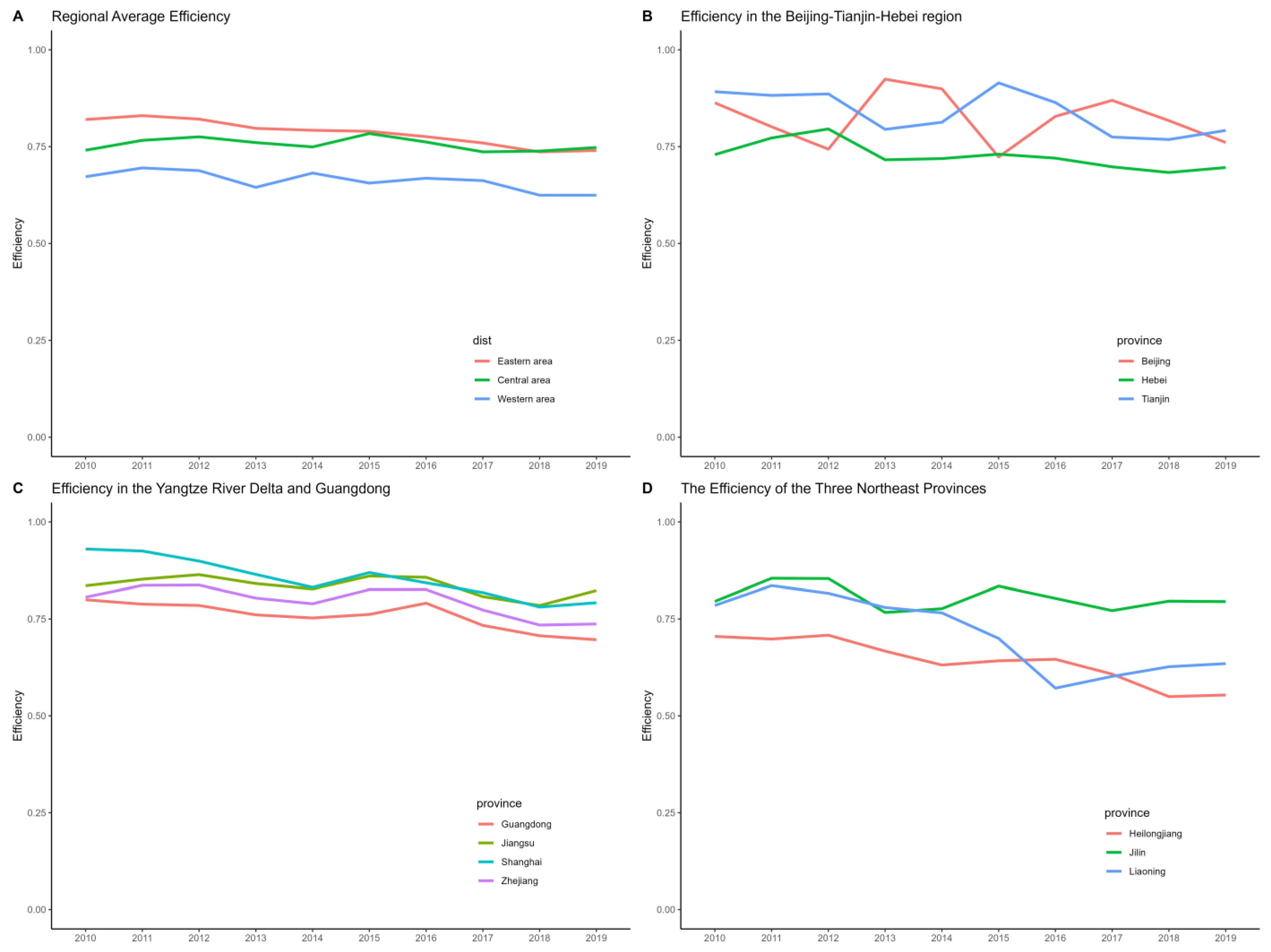
We further analyzed the efficiency change trends of various regions during this period. Figure 3A displays the average efficiency changes of the three regions, highlighting the temporal trends. The figure illustrates a gradual decline in average efficiency in the eastern region, contrasted with a slow increase in the efficiency of the central region. This trend mirrors shifts in China’s industrial distribution over the years, indicating a gradual reallocation of industrial development focus from the eastern to the central regions.

Figure 3B depicts the changes within the Beijing-Tianjin-Hebei triangle area over this period. From 2010 to 2019, Beijing and Tianjin’s production efficiency showed significant fluctuations, in contrast to Hebei’s relatively stable efficiency. Notably, Beijing’s efficiency dipped in 2012, 2015, and 2019. A significant factor in Beijing’s efficiency decline is the underutilization of its expanding capital stock. By examining the raw data, we found that Beijing’s capital stock experienced substantial growth in these three years, increasing by 817.56 billion, 802.99 billion, and 265.05 billion yuan (in constant prices), with the first two increases being nearly 15%. Meanwhile, Beijing’s gross industrial output did not experience significant growth. This indicates that delays in production startup or year-end completions of new factories likely contributed to Beijing’s reduced efficiency. Tianjin’s case differs from Beijing’s. The reason for Tianjin’s lower production efficiency in 2013 is due to the growth of its capital stock by 948.98 billion yuan (in constant prices). Tianjin’s efficiency decline in 2017 can be attributed to supply-side reform policies, leading to a significant capital stock decrease. In 2017, Tianjin’s capital stock and total output value saw reductions of 1845.49 billion yuan and 8771.15 billion yuan, respectively, the latter constituting roughly a quarter of 2016’s total output.

Figure 3C reveals minimal fluctuations in productivity trends within the Yangtze River Delta region (Shanghai, Zhejiang, Jiangsu), indicating consistency. This consistency suggests that productivity in the region grew steadily, in a balanced and mutually reinforcing manner. Likewise, Guangdong’s productivity trend mirrored that of the Yangtze River Delta, indicating synchronized development patterns among major coastal cities.

Figure 3D illustrates a gradual decline in production efficiency in Heilongjiang, contrasted with an increase in Jilin, among the three northeastern provinces. This trend reflects a significant shift in industrial emphasis within the northeast region. Beginning in 2016, Liaoning Province saw a notable decrease in output value, resulting in a marked reduction in production efficiency. One reason for this downturn is the previously overstated data in Liaoning Province. In 2016, Liaoning disclosed its actual GDP as 2203.7 billion yuan, reflecting a 670.5 billion yuan reduction from 2015—an exaggeration rate of 23.3%. Following this disclosure, Liaoning’s national GDP ranking fell from 10th to 14th. Subsequently, its growth rate remained among the lowest in the country for several years. Additionally, beginning in 2011, Liaoning has been focusing on developing its service industry, signifying a strategic adjustment in its development priorities.

5.3.2. The Analysis on Total Factor Energy Efficiency

From the total factor energy efficiency proposed by hu et al. [34], the total factor energy efficiency can be calculated as follows.

$$\mathrm{T}\mathrm{F}\mathrm{E}\mathrm{E}=\frac{\mathrm{T}\mathrm{a}\mathrm{r}\mathrm{g}\mathrm{e}\mathrm{t} \mathrm{E}\mathrm{n}\mathrm{e}\mathrm{r}\mathrm{g}\mathrm{y} \mathrm{I}\mathrm{n}\mathrm{p}\mathrm{u}\mathrm{t}}{\mathrm{A}\mathrm{c}\mathrm{t}\mathrm{u}\mathrm{a}\mathrm{l} \mathrm{E}\mathrm{n}\mathrm{e}\mathrm{r}\mathrm{g}\mathrm{y} \mathrm{I}\mathrm{n}\mathrm{p}\mathrm{u}\mathrm{t}}$$

(14)

In the SBM game cross-efficiency model, the total factor energy efficiency is calculated as follows.

$$\mathrm{T}\mathrm{F}\mathrm{E}{\mathrm{E}}_{\mathrm{d}}=1-\frac{\frac{1}{\mathrm{N}}\left({\sum }_{\mathrm{i}}^{\mathrm{N}}{\mathrm{s}}_{\mathrm{i}\mathrm{d}}^{\left(\mathrm{k}\right)\mathrm{e}-}\right)}{{\mathrm{x}}_{\mathrm{d}}^{\mathrm{e}}},\mathrm{k}=1,2,\dots ,\mathrm{N}$$

(15)

The total factor energy efficiency of 30 provinces and cities in China is shown in

Table 6. Total factor energy efficiency results by province.

Area	2010	2011	2012	2013	2014	2015	2016	2017	2018	2019	Average	Rank
Eastern	0.7538	0.7750	0.7876	0.6542	0.6428	0.7637	0.6744	0.6184	0.6197	0.6619	0.6952
Beijing	0.9735	0.9881	0.9889	0.9933	0.9944	0.9931	0.9958	0.9957	0.9958	0.9926	0.9911	1
Fujian	0.6469	0.6646	0.7037	0.7511	0.6462	0.7502	0.6682	0.7036	0.7626	0.8259	0.7123	7
Guangdong	0.9763	0.9028	0.9235	0.8548	0.8152	0.9585	0.8878	0.8151	0.8358	0.8824	0.8852	2
Hainan	0.7219	0.7133	0.5902	0.2375	0.4735	0.4015	0.3703	0.4740	0.2689	0.3049	0.4556	18
Hebei	0.3041	0.4137	0.4931	0.2354	0.2387	0.3856	0.3075	0.2538	0.2318	0.2951	0.3159	28
Jiangsu	0.8314	0.8542	0.9250	0.8169	0.7675	0.9324	0.8641	0.7361	0.7604	0.8002	0.8288	4
Liaoning	0.4735	0.6195	0.5843	0.4695	0.4346	0.4455	0.2547	0.1856	0.2294	0.3269	0.4024	21
Shandong	0.6669	0.6835	0.7296	0.7494	0.6731	0.8651	0.7500	0.6869	0.6790	0.5985	0.7082	8
Shanghai	0.9517	0.9340	0.9493	0.7757	0.7093	0.8852	0.7631	0.6966	0.7447	0.8018	0.8211	5
Tianjin	0.8256	0.8386	0.8435	0.4812	0.5316	0.8458	0.6866	0.4826	0.5106	0.5978	0.6644	10
Zhejiang	0.9201	0.9123	0.9329	0.8311	0.7872	0.9374	0.8707	0.7727	0.7982	0.8552	0.8618	3
Central	0.5065	0.5774	0.6090	0.5317	0.5221	0.6928	0.5855	0.5204	0.6105	0.6514	0.5807
Anhui	0.6270	0.6887	0.7576	0.6726	0.6607	0.8107	0.6665	0.6459	0.7244	0.7308	0.6985	9
Henan	0.4611	0.5847	0.6800	0.7262	0.7037	0.9119	0.8063	0.7282	0.7593	0.8168	0.7178	6
Heilongjiang	0.5249	0.5365	0.5495	0.3284	0.3098	0.5323	0.3580	0.2625	0.3421	0.3453	0.4089	20
Hubei	0.5106	0.6145	0.5365	0.6630	0.6163	0.7623	0.6613	0.6042	0.7141	0.7885	0.6471	12
Hunan	0.4834	0.5272	0.5832	0.6399	0.5864	0.7085	0.5774	0.5676	0.7272	0.7971	0.6198	13
Jilin	0.5109	0.6662	0.6800	0.3981	0.4153	0.6588	0.5788	0.4801	0.5949	0.6066	0.5590	15
Jiangxi	0.6092	0.6512	0.6837	0.5865	0.5364	0.7000	0.6618	0.6401	0.7316	0.8029	0.6603	11
Shanxi	0.3246	0.3500	0.4015	0.2392	0.3478	0.4581	0.3735	0.2349	0.2900	0.3229	0.3342	26
Western	0.4181	0.4923	0.4720	0.3071	0.4154	0.4667	0.4229	0.3876	0.3473	0.3915	0.4121
Gansu	0.3892	0.6370	0.5804	0.2422	0.4274	0.4257	0.4082	0.2646	0.2628	0.2753	0.3913	23
Guangxi	0.4070	0.4170	0.4595	0.4447	0.3854	0.4768	0.4107	0.3904	0.4632	0.5384	0.4393	19
Guizhou	0.2836	0.2880	0.2923	0.2630	0.2963	0.5623	0.4811	0.4078	0.3983	0.4611	0.3734	24
Inner Mongolia	0.5829	0.7315	0.6195	0.2333	0.4947	0.3873	0.3233	0.2952	0.1429	0.1569	0.3968	22
Ningxia	0.2392	0.2590	0.3010	0.1745	0.3183	0.2682	0.2620	0.2740	0.1504	0.1647	0.2411	30
Qinghai	0.3869	0.5598	0.4317	0.1831	0.3672	0.2902	0.2860	0.2955	0.1615	0.1773	0.3139	29
Shaanxi	0.5790	0.6434	0.7193	0.4116	0.4598	0.6671	0.5566	0.5148	0.4863	0.5516	0.5589	16
Sichuan	0.5102	0.4876	0.5085	0.3605	0.5250	0.5948	0.5263	0.4708	0.5683	0.6437	0.5196	17
Xinjiang	0.4794	0.5386	0.3914	0.1614	0.3156	0.3097	0.2923	0.3635	0.1937	0.2084	0.3254	27
Yunnan	0.3316	0.4276	0.4227	0.2434	0.3966	0.4046	0.3604	0.3693	0.3064	0.3472	0.3610	25
Chongqing	0.4098	0.4260	0.4656	0.6601	0.5829	0.7468	0.7454	0.6173	0.6864	0.7823	0.6123	14

. Overall, energy efficiency is still the highest in eastern cities, followed by central cities, and the lowest in western cities. From 2010 to 2019, Beijing, Guangdong, Zhejiang, Jiangsu, and Shanghai had relatively high average total factor energy efficiencies, all exceeding 0.80. In contrast, Ningxia, Qinghai, Xinjiang, Gansu, and Shanxi had lower energy efficiencies, all below 0.35, indicating significant room for improvement. Most provinces and cities show an upward trend in energy efficiency, although the changes are relatively stable.

Shanghai and Shandong have experienced a declining trend in energy efficiency. Among them, Shanghai decreased from 0.9517 to 0.8018, a drop of 0.1499, or 15.75%. The slow decline in Shanghai is due to the gradual decrease in industrial capital stock and labor since 2015, while energy input increased. As a result, Shanghai improved its capital and labor utilization efficiency while experiencing a decrease in energy efficiency. Shandong’s decline in energy efficiency is consistent with that of Shanghai.

Most provinces maintain stable or improved industrial energy efficiency; meanwhile, most provinces also maintain stable or decreased production efficiency. This reflects China’s growing focus on environmental and energy improvements in industrial development.

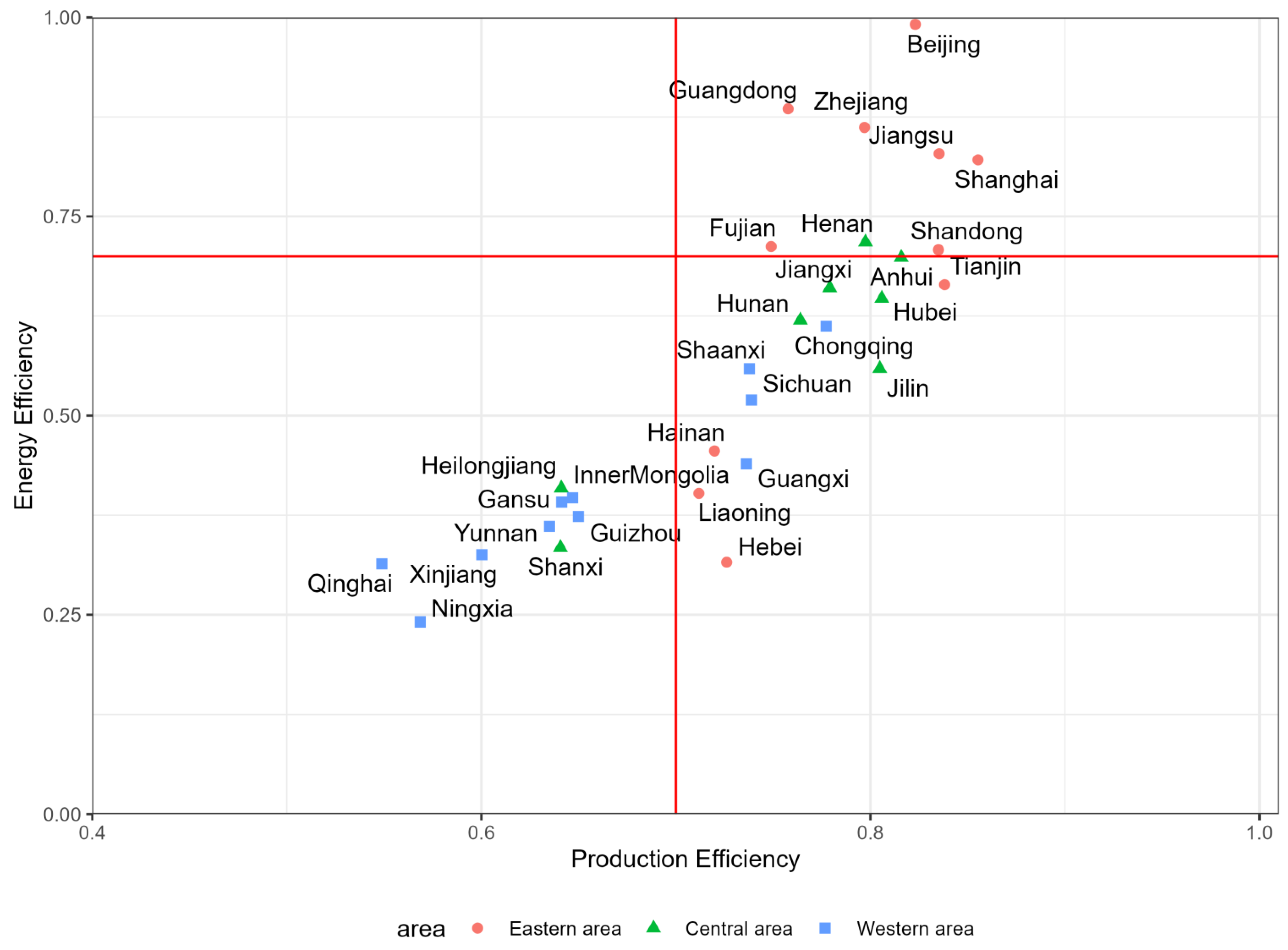
In Figure 4, we present a comprehensive analysis by integrating the average production efficiency and total factor energy efficiency for every province. Subsequently, we categorized the decision units into four distinct groups using a dividing line of 70%. The first group, located in the upper-left quadrant, represents DMUs with low production efficiency but high energy efficiency. In particular, factors such as labor productivity and capital utilization require significant improvement. However, we acknowledge that decision units in this category are less prevalent due to the high dependence of energy efficiency on labor productivity and capital utilization.

The second group, located in the upper-right quadrant, represents DMUs with exemplary performance in terms of both productivity and total factor energy efficiency. This group serves as a model for other decision-making units to learn from. Notably, provinces and cities such as Guangdong, Beijing, Jiangsu, Zhejiang, and Shanghai demonstrate remarkable performance in this category.

In contrast, the third group, located in the lower-left quadrant, represents DMUs with low performance in both production efficiency and total factor energy efficiency. With significant room for improvement, provinces and cities such as Qinghai, Yunnan, Shanxi, Ningxia, and Xinjiang display significant potential for efficiency enhancements.

The fourth type of region is the bottom right corner region, where the DMUs have a relatively high production efficiency but low total factor energy efficiency. These regions are characterized by a focus on production without considering environmental protection, prioritizing economic development. Therefore, they are called high-consumption economic areas.

There continue to be significant disparities in both production efficiency and energy efficiency levels among the eastern, central, and western regions. In the western region, production efficiency is below 0.80, and energy efficiency ratings fall under 0.70, with four provinces even recording ratings lower than 0.35. In contrast, in the eastern region, only three provinces have production efficiencies below 0.75. These provinces also have higher energy efficiencies, none dropping below 0.60. The central region demonstrates a spectrum of production efficiency and energy efficiency ranks, with some provinces showing elevated energy efficiency and production efficiency levels and others reporting lower rates. Notably, Guangdong in the Pearl River Delta region exhibits high levels of both production efficiency and total factor energy efficiency. Similarly, Shanghai, Zhejiang, and Jiangsu in the Yangtze River Delta area also demonstrate high levels of these efficiencies. The data results align with our real-life impressions. In these economically developed regions, high production efficiency is required to cover higher costs and increased industry competition. The total factor energy efficiency is related to government policies. Guangdong and Beijing have stricter energy and carbon emission regulations, leading to higher total factor energy efficiency in these areas.

5.4. Robustness Analysis

To test the robustness of the results, this paper controls the data and performs comparative analysis. Using the same data, we apply the traditional SBM input-oriented model and two cross-efficiency input-oriented models to analyze production efficiency.

Table 7. Comparison of the results of the 2010 data in different models.

Province	(1)		(2)		(3)		(4)
	Our Model	Rank	Tone	Rank	Doyle and Green	Rank	Lim and Zhu	Rank
Beijing	0.8632	3	1.0000	1	0.8792	5	0.8394	5
Fujian	0.7247	20	1.0000	1	0.6968	17	0.6721	16
Guangdong	0.7997	9	1.0000	1	0.7163	16	0.7034	12
Hainan	0.8384	4	1.0000	1	0.7803	10	0.2126	29
Hebei	0.7295	19	0.6577	16	0.8024	8	0.7695	7
Jiangsu	0.8353	5	1.0000	1	0.8860	4	0.8705	4
Liaoning	0.7851	12	0.7449	11	0.8342	6	0.8088	6
Shandong	0.8161	6	1.0000	1	0.9285	3	0.9103	2
Shanghai	0.9300	1	1.0000	1	0.9620	1	0.9420	1
Tianjin	0.8919	2	1.0000	1	0.9426	2	0.9026	3
Zhejiang	0.8064	7	0.9224	10	0.7413	12	0.7256	11
Anhui	0.8017	8	0.6981	13	0.7271	14	0.6953	14
Henan	0.7394	18	0.6949	14	0.7657	11	0.7381	10
Heilongjiang	0.7052	23	0.5376	23	0.5567	23	0.5113	22
Hubei	0.7735	13	0.6024	20	0.6706	18	0.6435	17
Hunan	0.7462	17	0.6725	15	0.7329	13	0.6983	13
Jilin	0.7955	10	0.7253	12	0.8121	7	0.7609	8
Jiangxi	0.7607	15	1.0000	1	0.7981	9	0.7576	9
Shanxi	0.6042	27	0.4444	29	0.5050	27	0.4709	24
Gansu	0.6419	26	0.4941	27	0.5163	26	0.4237	26
Guangxi	0.7098	22	0.5718	22	0.6222	22	0.5731	21
Guizhou	0.5340	30	0.4294	30	0.4406	29	0.3580	27
Inner Mongolia	0.7712	14	0.6433	17	0.7210	15	0.6809	15
Ningxia	0.5741	29	0.5099	26	0.4909	28	0.2671	28
Qinghai	0.5819	28	0.5349	24	0.4291	30	0.0677	30
Shaanxi	0.7910	11	0.6268	18	0.6613	19	0.6155	19
Sichuan	0.7546	16	0.5940	21	0.6526	21	0.6262	18
Xinjiang	0.6851	24	0.5114	25	0.5399	25	0.4392	25
Yunnan	0.6440	25	0.4889	28	0.5442	24	0.4727	23
Chongqing	0.7100	21	0.6200	19	0.6591	20	0.6085	20

displays the production efficiency values obtained in 2010 using different input-oriented models. The first model is the SBM game cross-efficiency model proposed in this study; the second model is the SBM model proposed by Tone [28]; the third model is the one proposed by Doyle and Green [1]; and the fourth model is proposed by Lim and Zhu [13].

From Table 7, it can be seen that the results of the model proposed in this study are similar to those of the other two cross-efficiency models, which confirms the robustness of the results. In addition, the traditional SBM model tends to assign efficiency values of 1 to most decision-making units, making comparison impossible. Moreover, the traditional SBM model has some efficiency value misestimations, such as Hainan Province’s efficiency value of 1, despite the province’s weak industrial base. Cross-efficiency models greatly outperform the traditional SBM model in this regard. The model proposed in this study goes even further, taking into account both slack variables and competitiveness among decision-making units.

From Figure 5, it is evident that the kernel density plots for all models are predominantly concentrated between 0.5 and 0.9. The model introduced in this study exhibits a more concentrated distribution within this range compared to the others. A distinctive characteristic of the proposed model is its elevated minimum limit and the infrequent occurrence of DMUs attaining the maximum efficiency score of 1. This elevated minimum efficiency reflects the model’s capability to optimize its efficiency, considering the efficiency levels of other DMUs. The rarity of DMUs reaching an efficiency score of 1 suggests that the model’s efficiency calculations provide superior comparability, enabling a more accurate ranking of DMUs by production efficiency.

As evidenced by

Table 8. The results of the correlation tests for all models.

	Mean	SD	Our Model	Tone	Doyle and Green	Lim and Zhu
Our model	0.7448	0.0945	1.0000
Tone	0.7242	0.2076	0.8001 ***	1.0000
Doyle and Green	0.7005	0.1498	0.9137 ***	0.8318 ***	1.0000
Lim and Zhu	0.6225	0.2133	0.7554 ***	0.6096 ***	0.8512 ***	1.0000

Note: *** indicates significance at the 0.001 level.

, there exists a notably high correlation between the model introduced in this study and the outcomes derived from alternative models. This suggests that the efficiency estimates of the DMUs generated by the proposed model exhibit minimal deviation. Integrating this with prior analyses allows for the conclusion that the model yields more precise rankings of DMU production efficiency. Hence, the calculated outcomes of the proposed model are robust and surpass those derived from other models.

6. Conclusions

This paper introduces an SBM game cross-efficiency model incorporating undesirable outputs. This model enhances the SBM cross-efficiency framework and integrates aspects of game cross-efficiency. It includes non-oriented models, input-oriented models, and output-oriented models. Different oriented models are used for different evaluation purposes. The non-oriented model balances input and output, making it suitable for the goal orientation of simultaneous economic development, energy conservation, and emission reduction. The input-oriented model focuses on saving input, while the output-oriented model emphasizes expanding desirable output and reducing emissions.

These models offer distinct advantages over traditional models. First, the model ensures all decision units achieve maximum efficiency with others’ efficiencies held constant, circumventing the issue of solution uniqueness in cross-efficiency models. Second, it enables a more precise ranking of decision units, preventing scenarios where numerous DMUs with an efficiency score of 1 remain incomparable. Finally, it weights the efficiencies of all decision units based on efficiency values, using various frontier decision units as benchmarks. Consequently, these models offer more stringent frontier surface analyses and unbiased efficiency assessments compared to Kao and Liu’s SBM cross-efficiency model [2].

In the empirical analysis, this study uses the data of industrial enterprises above a designated size in 30 provinces and cities in China from 2010 to 2019. We find that eastern provinces generally have higher production efficiency and energy efficiency, such as Guangdong, Beijing, Jiangsu, Zhejiang, and Shanghai, which are the benchmarks for other provinces and cities to learn from. Central provinces show a polarization: either they have relatively high production and energy efficiency, such as Henan, Jiangxi, and Hunan; or they have relatively low production and energy efficiency, like Shanxi and Heilongjiang. Most western provinces have relatively low production and energy efficiency, and overall improvements are needed, such as in Qinghai, Yunnan, Ningxia, and Xinjiang. The average production efficiency is the highest in the east, the second in the middle, and the lowest in the west. The average production efficiency in the eastern region is gradually declining, falling by about 10% in 10 years, while the production efficiencies in the central and western regions remain stable.

The model in this paper still has a certain limit. On the one hand, the model proposed in this paper does not consider the intertemporal comparison and is still based on the static game, and there is still room for improvement. On the other hand, this paper does not involve the price factor. The model emphasizes technical efficiency rather than cost efficiency. However, if cost efficiency is prioritized, a more accurate assessment of efficiency can be achieved. Unfortunately, since price data are often difficult to obtain, this will be challenging.

References

1. Doyle, J.; Green, R. Efficiency and Cross-Efficiency in DEA: Derivations, Meanings and Uses. J. Oper. Res. Soc. 1994, 45, 567–578. [Google Scholar] [CrossRef]
2. Kao, C.; Liu, S.-T. A Slacks-Based Measure Model for Calculating Cross Efficiency in Data Envelopment Analysis. Omega 2020, 95, 102192. [Google Scholar] [CrossRef]
3. Liang, L.; Wu, J.; Cook, W.D.; Zhu, J. The DEA Game Cross-Efficiency Model and Its Nash Equilibrium. Oper. Res. 2008, 56, 1278–1288. [Google Scholar] [CrossRef]
4. Charnes, A.; Cooper, W.W.; Rhodes, E. Measuring the Efficiency of Decision Making Units. Eur. J. Oper. Res. 1978, 2, 429–444. [Google Scholar] [CrossRef]
5. Sexton, T.R.; Silkman, R.H.; Hogan, A.J. Data Envelopment Analysis: Critique and Extensions. New Dir. Program Eval. 1986, 1986, 73–105. [Google Scholar] [CrossRef]
6. Wu, J.; Sun, J.; Liang, L. Cross Efficiency Evaluation Method Based on Weight-Balanced Data Envelopment Analysis Model. Comput. Ind. Eng. 2012, 63, 513–519. [Google Scholar] [CrossRef]
7. Wang, Y.-M.; Chin, K.-S.; Wang, S. DEA Models for Minimizing Weight Disparity in Cross-Efficiency Evaluation. J. Oper. Res. Soc. 2012, 63, 1079–1088. [Google Scholar] [CrossRef]
8. Wang, Y.-M.; Chin, K.-S. The Use of OWA Operator Weights for Cross-Efficiency Aggregation. Omega 2011, 39, 493–503. [Google Scholar] [CrossRef]
9. Wu, J.; Chu, J.; Sun, J.; Zhu, Q.; Liang, L. Extended Secondary Goal Models for Weights Selection in DEA Cross-Efficiency Evaluation. Comput. Ind. Eng. 2016, 93, 143–151. [Google Scholar] [CrossRef]
10. Carrillo, M.; Jorge, J.M. An Alternative Neutral Approach for Cross-Efficiency Evaluation. Comput. Ind. Eng. 2018, 120, 137–145. [Google Scholar] [CrossRef]
11. Kao, C.; Liu, S.-T. Cross Efficiency Measurement and Decomposition in Two Basic Network Systems. Omega 2019, 83, 70–79. [Google Scholar] [CrossRef]
12. Liu, H.; Song, Y.; Yang, G. Cross-Efficiency Evaluation in Data Envelopment Analysis Based on Prospect Theory. Eur. J. Oper. Res. 2019, 273, 364–375. [Google Scholar] [CrossRef]
13. Lim, S.; Zhu, J. DEA Cross-Efficiency Evaluation under Variable Returns to Scale. J. Oper. Res. Soc. 2015, 66, 476–487. [Google Scholar] [CrossRef]
14. Lim, S. Minimax and Maximin Formulations of Cross-Efficiency in DEA. Comput. Ind. Eng. 2012, 62, 726–731. [Google Scholar] [CrossRef]
15. Lin, R. Cross-Efficiency Evaluation Capable of Dealing with Negative Data: A Directional Distance Function Based Approach. J. Oper. Res. Soc. 2020, 71, 505–516. [Google Scholar] [CrossRef]
16. Portela, M.C.A.S.; Thanassoulis, E.; Simpson, G. Negative Data in DEA: A Directional Distance Approach Applied to Bank Branches. J. Oper. Res. Soc. 2004, 55, 1111–1121. [Google Scholar] [CrossRef]
17. Örkcü, H.H.; Özsoy, V.S.; Örkcü, M.; Bal, H. A Neutral Cross Efficiency Approach for Basic Two Stage Production Systems. Expert Syst. Appl. 2019, 125, 333–344. [Google Scholar] [CrossRef]
18. Banker, R.D. A Game Theoretic Approach to Measuring Efficiency. Eur. J. Oper. Res. 1980, 5, 262–266. [Google Scholar] [CrossRef]
19. Hao, G.; Wang, S.; Chen, H.; Zhang, W.; Jiang, S.; Li, L. Optimum Energy Efficiency in Lunar In-Situ Water Ice Utilization. Acta Astronaut. 2023, 207, 307–315. [Google Scholar] [CrossRef]
20. Nakabayashi, K.; Tone, K. Egoist’s Dilemma: A DEA Game. Omega 2006, 34, 135–148. [Google Scholar] [CrossRef]
21. Xie, B.-C.; Gao, J.; Zhang, S.; Pang, R.-Z.; Zhang, Z. The Environmental Efficiency Analysis of China’s Power Generation Sector Based on Game Cross-Efficiency Approach. Struct. Chang. Econ. Dyn. 2018, 46, 126–135. [Google Scholar] [CrossRef]
22. Chen, W.; Wu, F.; Geng, W.; Yu, G. Carbon Emissions in China’s Industrial Sectors. Resour. Conserv. Recycl. 2017, 117, 264–273. [Google Scholar] [CrossRef]
23. Yang, Z.; Wei, X. The Measurement and Influences of China’s Urban Total Factor Energy Efficiency under Environmental Pollution: Based on the Game Cross-Efficiency DEA. J. Clean. Prod. 2019, 209, 439–450. [Google Scholar] [CrossRef]
24. Wu, J.; Liang, L.; Chen, Y. DEA Game Cross-Efficiency Approach to Olympic Rankings. Omega 2009, 37, 909–918. [Google Scholar] [CrossRef]
25. Li, F.; Zhu, Q.; Liang, L. Allocating a Fixed Cost Based on a DEA-Game Cross Efficiency Approach. Expert Syst. Appl. 2018, 96, 196–207. [Google Scholar] [CrossRef]
26. Li, Y.; Li, F.; Emrouznejad, A.; Liang, L.; Xie, Q. Allocating the Fixed Cost: An Approach Based on Data Envelopment Analysis and Cooperative Game. Ann. Oper. Res. 2019, 274, 373–394. [Google Scholar] [CrossRef]
27. Wang, G.; Chao, Y.; Lin, J.; Chen, Z. Evolutionary Game Theoretic Study on the Coordinated Development of Solar Power and Coal-Fired Thermal Power under the Background of Carbon Neutral. Energy Rep. 2021, 7, 7716–7727. [Google Scholar] [CrossRef]
28. Tone, K. A Slacks-Based Measure of Efficiency in Data Envelopment Analysis. Eur. J. Oper. Res. 2001, 130, 498–509. [Google Scholar] [CrossRef]
29. Li, S.; Diao, H.; Wang, L.; Li, L. A Complete Total-Factor CO2 Emissions Efficiency Measure and “2030•60 CO2 Emissions Targets” for Shandong Province, China. J. Clean. Prod. 2022, 360, 132230. [Google Scholar] [CrossRef]
30. Guan, Y.; Shan, Y.; Huang, Q.; Chen, H.; Wang, D.; Hubacek, K. Assessment to China’s Recent Emission Pattern Shifts. Earths Future 2021, 9, e2021EF002241. [Google Scholar] [CrossRef]
31. Shan, Y.; Liu, J.; Liu, Z.; Xu, X.; Shao, S.; Wang, P.; Guan, D. New Provincial CO2 Emission Inventories in China Based on Apparent Energy Consumption Data and Updated Emission Factors. Appl. Energy 2016, 184, 742–750. [Google Scholar] [CrossRef]
32. Shan, Y.; Guan, D.; Zheng, H.; Ou, J.; Li, Y.; Meng, J.; Mi, Z.; Liu, Z.; Zhang, Q. China CO2 Emission Accounts 1997–2015. Sci. Data 2018, 5, 170201. [Google Scholar] [CrossRef] [PubMed]
33. Shan, Y.; Huang, Q.; Guan, D.; Hubacek, K. China CO2 Emission Accounts 2016–2017. Sci. Data 2020, 7, 54. [Google Scholar] [CrossRef] [PubMed]
34. Hu, J.-L.; Wang, S.-C. Total-Factor Energy Efficiency of Regions in China. Energy Policy 2006, 34, 3206–3217. [Google Scholar] [CrossRef]
Figure 1. Graphical representation of data. for Case 1 (A) and Case 2 (B). (Note: In both subfigures A (Case 1) and B (Case 2), the red dots represent the positions of the DMUs, with letters indicating the names of the DMUs. The solid black lines indicate the efficiency frontier. The red dashed lines are specifically drawn to highlight the difference in the position of DMU G between the two cases).
Systems 12 00078 g001
Figure 2. Achieving the best game cross-efficiency of the overall process for 11 regions in the eastern area.
Systems 12 00078 g002
Figure 3. Trends in the overall efficiencies in different regions and provinces from 2010 to 2019.
Systems 12 00078 g003
Figure 4. Ten-year average production efficiency and energy efficiency of each province. (Note: In this figure, red solid lines at x = 0.7 and y = 0.7 demarcate the threshold for acceptable efficiency levels, with efficiency values of 0.7 or higher considered satisfactory.)
Systems 12 00078 g004
Figure 5. The kernel density plots for all models.
Systems 12 00078 g005