Abstract
Project risk management (PRM) involves identifying risks, assessing their impact, and developing a contingency plan. A structured contingency management (CM) approach prevents subjective biases in analyzing risks and developing responses. Previous studies have either focused on improving the accuracy of risk estimates or analyzed, from a qualitative perspective, the relationships between perceived risk and project performance. This study aimed to improve PRM by providing a risk-perception-based contingency management framework (CMF). The CMF guides contingency depletion based on two short- and long-term cost overrun indicators and their respective thresholds. Thresholds and the initial contingency reserve amount are determined by applying the Monte Carlo method to a stochastic, discrete-event, finite-horizon, dynamic project simulation model. The study developed the CMF through a structured approach, validating the simulation model on eight specific project configurations. The results prove that the framework can be applied to any project, shaping the risk response strategy. This study contributes to PRM by explaining the relationships between risk perception and risk responses and providing a prescriptive CM tool.
1. Introduction
Effective project risk management (PRM) is crucial to project success. PRM involves identifying potential risks, evaluating their impact on the project system, and implementing responses to increase the likelihood of meeting project objectives [1]. The weight of PRM increases with project complexity, as complex projects face a wider range of potential risks [2].
In projects, risks can lead to both direct and indirect cost overruns. Direct cost overruns arise when the actual cost of project activities exceeds their budget, often due to price fluctuations, scope changes, or inefficiencies during execution [3,4]. Instead, indirect cost overruns stem from the cascading effects of risks on the project system, such as schedule delays or disruptions triggering overtime or contract penalties [5].
Cost overruns trigger short- and long-term concerns in project managers about not respecting the project budget. Short-term (ST) concern arises from the deviation between the actual cost of work performed and its budgeted value. Conversely, long-term (LT) concern arises from the deviation between the project cost estimate at completion and the available budget, encompassing the planned budget and contingency reserve.
In PRM, the contingency reserve (CR) is a financial buffer within the project cost baseline to address known unknown risks [6]. Project managers utilize the CR to fund responses to materialized risks that lead to cost overruns. The CR is determined by the contingency plan, which outlines the criteria for assessing risk responses, including whether to implement them, how, and to what extent.
PRM success comes down to effective contingency management (CM). Without a contingency plan, risk responses are determined based on project managers’ perceptions [7], which include both attitude and appetite. However, risk perception is influenced by organizational values and personal experiences, making it inherently subjective [8]. Subjective CM exposes the project to additional risks that may affect project success [9]. Therefore, integrating expert judgment with data-driven decisions is crucial to effective CM. By leveraging data, managers can make informed decisions supported by concrete evidence and robust analysis [10].
Despite the extensive literature on PRM, few studies have provided objective frameworks to guide CM. While most works have focused on improving the accuracy of risk estimates, they overlook or address only qualitatively the implications of project managers’ risk perceptions on PRM. Therefore, it is essential to follow a structured approach to CM that prevents subjective behaviors.
This study’s objective is twofold. Firstly, it explains the relationship between short- and long-term cost overruns, how project managers perceive them, and how they can react. Secondly, it aims to model risk perception, provide the criteria for developing risk responses, and implement both within a contingency management framework (CMF) to minimize short- and long-term concerns for cost overruns throughout project execution while ensuring the complete depletion of the CR. The CMF applies the Monte Carlo (MC) method to a stochastic, discrete-event, finite-horizon, dynamic project simulation model for evaluating the combinations of initial CR level and response thresholds that optimize contingency spending. In the CMF, risk responses consist of using part of the CR to reduce the increase in the project’s actual cost, thereby reducing both the perceived overrun and the cost variance at project completion.
This paper is organized as follows. Section 1 provided the background of the study and its objectives. Section 2 reviews previous studies on contingency estimation models, CM models, risk control thresholds, and risk perception in project management. Section 3 describes the proposed CM framework. Section 4 provides the results of the framework testing on synthetic project configurations, which are then discussed in Section 5. Lastly, Section 6 lists the limitations of the study and the avenues for future research.
2. Literature Review
Literature on PRM is vast and encompasses a comprehensive range of research topics, including identifying and evaluating risks, CM, establishing risk response thresholds, and analyzing the relationship between PRM and project performance. While the review provides a brief overview of the first category, it delves into a more in-depth exploration of the latter three areas.
Project risk identification and evaluation studies focus on determining the appropriate size of the CR. To this end, two distinct approaches are employed: deterministic and probabilistic [11]. In deterministic approaches, project risks are characterized by predefined probabilities and impact values [12]. In contrast, probabilistic approaches recognize the inherent uncertainty associated with project risks, assigning probability distributions to each level of potential impact [13].
CM studies have proposed different models to guide the depletion of CR throughout project execution. Ford [14] built a dynamic behavioral simulation model to test how different CM strategies impact project performance. Their findings showed that a passive strategy performs better under critical conditions, whereas an aggressive strategy is more robust to changes. Barraza and Bueno [15] proposed a heuristic approach based on MC simulation for determining whether to intervene and to what extent according to the activities’ cost and cost variance. The study concluded that the optimal CM strategy is not predetermined but depends on project characteristics and the project manager’s subjective behavior. Moselhi and Salah [16] and Salah and Moselhi [17] developed fuzzy-set-based CM methods for determining contingency depletion based on periodically allocated contingency and uncertainty measures. Their results demonstrated the superior capabilities of the proposed methods compared to MC. Xie et al. [12] applied a value-at-risk method to update project contingencies as the project progresses, implementing newly available information inferred from monitoring data. The method shifts the focus from risks and their magnitude to daily cost and earnings, overcoming the problem of correlation between risks. Eldosouky et al. [18] proposed a three-round approach for drawing upon contingency based on monitoring project progress metrics, relying on earned value management (EVM) metrics to monitor and control project contingencies. Hammad et al. [19] developed a heuristic-based CM method working at the activity level, which was later improved by Hammad et al. [20] by specifying that the allocated amount to each activity depends on its weight in the project cost, uncertainty, and criticality. Traynor and Mahmoodian [21] recommended MC simulation for contingency management, guiding activity-level depletion of their assigned cost and time buffers.
Several studies have implemented control thresholds within the project system based on preexisting or new metrics and indicators to capture deviations in performance proactively by generating early warnings. Kim et al. [22] introduced risk thresholds, evaluated through the value-at-risk concept, which would trigger if the profit ratio of the affected work package influences the project profit. Pajares and López-Paredes [23] introduced two monitoring metrics, namely, the cost control index and schedule control index, whose values determine whether early decisions should be made. Colin and Vanhoucke [24] developed a statistical project control procedure to set tolerance limits in the traditional monitoring indicators for determining whether the deviations from the performance measurement baseline are related to risk materializing. Colin et al. [25] introduced two multivariate control metrics, namely, and , obtained through MC simulation to set statistical tolerance limits. Kim [26] presented a quantitative method for establishing dynamic control thresholds depending on the project objectives’ overall progress and degree of achievability. Ballesteros-Pérez et al. [27] developed two schedule monitoring metrics, and , of which exceeding determines performance not under control. Kim and Pinto [28] investigated the predictive power of project cost data as an early indicator of the cost overrun probability in risk management. Chen et al. [29] adopted the Bayesian approach to determine the expected distributions of the tolerance limits of the project schedule metrics.
Many works have adopted system dynamics (SD) tools to model the relationships between PRM and project performance. Rodrigues [30] analyzed the feedback loops between risks, risk effects, and the project system, highlighting SD’s potential to improve response planning. Chritamara et al. [31] used SD modeling to incorporate sub-systems and their relationships in D/B construction projects to simulate how the system reacts to risks and different policies. Wang et al. [32] claimed traditional PRM techniques to be inappropriate when dealing with high uncertainty and dynamic project risks, suggesting SD for identifying risks and developing responses. Howick et al. [33] analyzed the indirect consequences of disruptions and delays, showing both disruption and delay feedback on themselves causing further disruptions and delays. Ding et al. [34] designed a PRM framework based on social network analysis and SD, simulating risk mitigation actions at the organizational level. Wang and Yuan [35] took a holistic view to investigate the effects of dynamic risk interactions on a schedule delay in infrastructure projects. Leon et al. [36] developed an SD model to simulate the complexities among interdependent variables and forecast their dynamics over time, simulating four possible intervention scenarios.
SD has also been used to demonstrate that project control processes are affected by risk perception [37]. The decision of when and how to spend the contingency budget depends significantly on risk perception [17]. Risk perception influences assessing risks and developing responses based on individual experiences of intuitive judgment and subjective cognition [38,39]. Qualitative perspectives have been embraced for evaluating the possibility of occurring risks, considering the dynamics behind the perception and response to a schedule delay. This leads to the employees experiencing low productivity, lower morale, and increased pressure due to work overload [8]. While this literature helps characterize the relationship between human perception and project risk, approaches that link risk perception with CM are still lacking.
Among the different studies analyzed, only two integrated risk perception and CM. De Marco et al. [40] proposed an SD-based CM model to simulate decision-making scenarios under different project conditions and behavioral pressures of senior managers and owners. The model considers multiple influences of the leading project participants in the problem. Their findings suggest that the CM strategy should be based on conflicting pressures to make preventive, risk-mitigating improvements or release the remaining CR as savings. The model was later improved by De Marco et al. [41] and applied to improve project cost estimates at completion, highlighting how the project CR expenditure behavior influences cost forecasts. Ayub et al. [42] developed a mathematical model that integrated project KPIs with future risk perception, enabling a quantitative approach to informal and subjective risk models. The cost contingency consumption trend analysis showed an S-curve pattern, with project managers holding back contingency in the early stages because of uncertainty. Steady consumption in the middle allowed them to address risks later, validating the cost impact of late changes.
Transitioning from project-level to organization and enterprise risk management entails various models outlined in the literature, which offer guidance on the timing and approach to developing risk responses. Noteworthy frameworks in this domain encompass ISO 31000 [43], the COSO ERM Framework [44], the DALI model [45], and the PRIMO FORTE framework [46].
Research Motivation
The literature review described different endeavors for improving PRM. Studies agree on (1) tailoring the CM strategy to specific projects, (2) utilizing simulation to account for the probabilistic nature of risks, and (3) considering the implications of risk perception on the decision-making processes. In this regard, this study proposes a CMF taking into account all the aspects above at once.
3. Research Methodology
The study developed the CMF, more specifically, the project execution simulation model, following a simplified version of the methodologies of Law [47] and Banks et al. [48], consisting of the following steps:
- Problem formulation and system configurations;
- Model definition;
- Model translation;
- Pilot runs;
- Model validation;
- Output data analysis;
- Discussion of results.
3.1. Problem Formulation and System Configurations
3.1.1. Problem Formulation
The CMF is intended as a prescriptive tool for driving CM while minimizing project managers’ exposure to risk perception. The CMF should determine, for each initial level of CR, the frequency and entity of risk responses. Such responses should be based on the difference between marginal and cumulative cost overruns and two predetermined thresholds. The CMF must apply to any project and be based on robust analysis; hence, the thresholds must be optimized by applying the MC method to a stochastic, discrete-event, finite-horizon, dynamic project execution simulation model. The simulation should undergo both verification and validation.
3.1.2. System Configurations
Model verification depends on the mathematical properties of the project execution simulation model. On the other hand, model validation requires testing it in several projects, which is not feasible because of the infinite number of possible project configurations. Hence, for the purpose of validation, this study employs synthetic data representing extreme project configurations. Suppose the CMF works in such extreme configurations. In this case, the CMF can be applied in any real project that has a configuration that falls between the extreme ones. This study defines project configurations based on the schedule, cost deviation, and correlation of the tasks.
Task schedule refers to the tasks’ start and end dates. Following the activity-based costing method [49], the task schedule determines the cumulative cost curve, which represents the total project cost as a function of time. Let and indicate the project budget at completion and planned duration, respectively. Then, the project cumulative cost curve can assume one of the four typical profiles in Figure 1 [50].
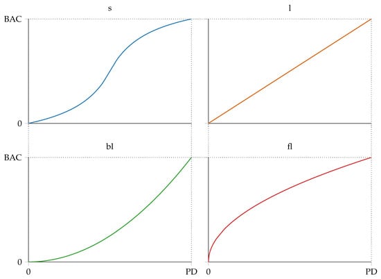
Figure 1.
Project cumulative cost curve typical profiles.
A task’s cost deviation is expressed using a probability density function (PDF) to account for potential risks Du et al. [51]. This function is derived by fitting a theoretical distribution to historical cost overrun data or by selecting an estimation method and gathering uncertainty factors for a sensitivity analysis. The resulting PDF values can be adjusted to accommodate additional risks that would substantially alter the task cost or to incorporate subjective assumptions.
Ideally, each task should have its cost deviation PDF. However, for verification and validation purposes, this study assumed all tasks’ cost deviation PDFs to be the same (in relative terms) [15,18]. Specifically, this study adopted the PERT distribution as PDF, i.e., a beta distribution extended to the domain [52].
Let x denote the task cost deviation. Then, Equation (1) provides the PDF of the PERT distribution:
where min is the x lower bound, max is the x upper bound, and are the shape parameters, and Beta is the beta function described by Equation (2),
Equation (3) provides the cumulative density function (CDF) of the PERT distribution:
where is the incomplete beta function and z is evaluated as per Equation (4),
By definition, the standard deviation () of the PERT distribution is equal to of the range. Therefore, the following equalities hold:
and
so that the distribution mean () is evaluated as per Equation (7),
while the variance () is given by Equation (8),
where is the distribution mode and is the distribution shape parameter. Figure 2 provides a graphical representation of the adopted PDF and CDF.
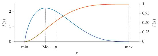
Figure 2.
Example PERTPDF (blue) and CDF (orange).
A task’s cost deviation correlation affects its cost deviation PDF. This study involves two correlation scenarios, namely, A and B. In Scenario A, all tasks are assumed to not be correlated. In scenario B, all tasks executed in the same time frame show the same relative cost deviation.
Table 1 summarizes the eight extreme configurations that serve to verify and validate the framework.

Table 1.
Project configurations codes.
3.2. Model Definition
The project execution simulation model is determined by combining SD conceptual modeling and the earned value management (EVM) [53] methodology. Figure 3 displays the project execution model as a causal loop diagram (CLD) to describe the relationships between EVM variables.
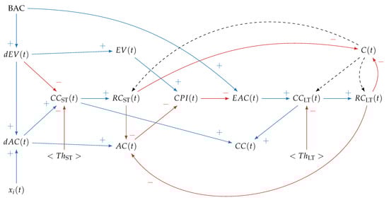
Figure 3.
Project monitoring variables CLD.
The CLD is defined as follows. The argument t, used as the simulation clock, indicates the tth project review, ranging from 0 (project start) to (project end). At any given t, tasks executed determine the increment in work performed (). Relating to the provides the increment in the budgeted cost of work performed (). In contrast, relating to the x determines the increment in actual cost () incurred to perform . The cumulative sum of provides the accrued earned value (), while the cumulative sum of provides the accrued actual cost ().
The difference between and the inflated , determined using the ST threshold (), provides the ST Concern for Cost Overruns indicator (). A corresponding Response to ST Cost Overruns () is developed if the current level of CR (C) allows for it. In the LT, the ratio of to provides the EVM cost performance index (), which is used to evaluate the project cost estimate at completion (). The difference between , BAC, and C, inflated by the LT threshold (), provides the LT Concern for Cost Overruns indicator (). A corresponding Response to LT Cost Overruns () is developed if the current C allows for it. Lastly, the overall Concern for Cost Overruns indicator () is theorized as a function of both and .
3.3. Model Translation
The CLD is translated into an analytical model describing the mathematical relationships between the EVM variables. Let denote the total number of tasks, each contributing equally to the project’s progress, and let i indicate the ith task. Then, Equation (9) holds.
Following EVM, progress is determined by assuming . Then, Equation (10) holds.
Let denote the number of tasks completed at time t, determined by the profiles displayed in Figure 1. Then, is determined using Equation (11).
In contrast, depends on both the task correlation and , which can be randomized by applying the inverse of Equation (3) to a random value generated through the uniform distribution, as in Equation (12).
In Scenario A, all project tasks are assumed to be independent; hence, is randomized per Equation (13).
In Scenario B, all tasks executed in the same t are assumed to show the same relative cost deviation. Therefore, is randomized per Equation (14).
The ratio of to provides the cost performance index (), as in Equation (17),
which is used as the projection factor to evaluate the project , as in Equation (18),
The Concern for ST Cost Overruns indicator () is determined per Equation (19):
where is non-negative, is the inflation factor, and is the ST threshold. The Response to ST Cost Overruns () is obtained by setting . Here, and indicate the respective variables after implementing the ST risk response. Solving by ,
leads to Equation (20),
where the response amount () is the smaller of the remaining contingency and the required non-negative amount that reduces to zero.
The Concern for LT Cost Overruns indicator () is determined per Equation (21):
where is non-negative, is the inflation factor, and is the LT threshold. The Response to LT Cost Overruns () is obtained by setting . Here, , , and indicate the respective variables after implementing the LT risk response. Solving by ,
leads to Equation (22),
where the response amount () is the smaller of the remaining contingency and the required non-negative amount that reduces to zero.
The project analytical model is fit within Algorithm 1, which evaluates all combinations of , , and optimizing CM.
| Algorithm 1: Contingency management framework optimization algorithm |
Data: , , Parameters: , , , , , , , , Result: Determine combinations that minimize  |
The algorithm is defined as follows. The parameter denotes the initial level of CR, i.e., . The parameters , , and denote the increment in , , and , respectively. An upper bound corresponds each parameter ( for , for , and for ). Iterations over are repeated until it reaches or until , triggering the first stop criterion (). Next, iterations over are repeated until it reaches . Finally, iterations over are repeated until it reaches or until the mean value of the residual C amount over the simulations () is reduced to almost zero (), triggering the second stop criterion ().
For each combination of and , the algorithm explores all possible values. The optimal combination is the one that minimizes the mean over the simulations of the mean Concern for Cost indicator () throughout the project duration. The algorithm stores the optimal combination as the variable and the optimal as the variable.
3.4. Pilot Runs
The algorithm was programmed from scratch in the Julia 1.8.1 programming language. Pilot runs (and later validation runs) were performed on an Acer Nitro AN 515-55 Intel(R) Core(TM) i7-10750H CPU; the run time was negligible.
3.4.1. Parameters Initialization
Simulation parameters were initialized arbitrarily. The number of simulations was set to 640 (i.e., ). The project duration was set to 24 (i.e., ), simulating a two-year-long project with monthly progress reviews. The budget was set to 100% (i.e., ). The total number of tasks was set to 100 (i.e., ).
Regarding the cost deviation PDF, the shape parameter was set to four (per traditional PERT) so that the mode () represented ∼66.67% of the distribution mean, i.e., so that . The mode was set to 100% (i.e., ), while the minimum and maximum were set to 80% (i.e., ) and 180% (i.e., ), respectively. As a result, the task cost tends to result in cost overruns (max 80% cost overruns) rather than savings (max 20% cost savings), and savings are usually smaller than cost overruns. Applying Equation (5) determines , whereas applying Equation (6) determines . On the other hand, applying Equation (7) determines , while applying Equation (8) determines .
3.4.2. Model Verification
The simulation model can be considered verified if it satisfies the central limit theorem (CLT) [54]. According to the CLT, the PDF of the project’s total cost deviation should conform to a normal distribution to which mean and variance correspond.
and
respectively. The CLT holds only if the random variables are iid (i.e., independent and identically distributed). In the simulation model, the random variables correspond to the tasks’ cost deviation PDFs and are iid only in the A configurations. However, if the only difference between Scenarios A and B is in the randomization of and the simulation model verifies the CLT in the A scenarios, then the B configurations should also be verified.
For the pilot runs, to verify whether the configurations met the requirements of the CLT, the number of simulations was set to 64,000 (i.e., ), the initial level of contingency was set to zero (i.e., ), and the thresholds were set to infinite (i.e., ), as never to trigger.
Table 2 presents the results of the pilot runs. All A configurations fulfill the conditions of the CLT since Equations (23) and (24) are satisfied. As a result, the model is considered verified.
Table 2.
Pilot runs’ cost at completion mean and variance.
3.5. Model Validation
Prior to conducting validation runs, the CR was bounded below zero () and above by 0.8 (). Following the pilot runs, the CLT could be applied to narrow the range of further to . This range is derived from the observation that a six-sigma interval covers approximately 99.7% of the possible outcomes. Based on this refined range of , it can be predicted that the model may not provide an optimal solution for values of below . Conversely, the CMF ensures that risks will always be mitigated for values of above .
For the validation runs, we set the following:
- ;
- ;
- .
4. Output Data Analysis
Table 3 presents the optimal configurations () determined by the CMF for each project configuration.
Table 3.
Optimal values of CMF parameters.
While the results depend on the algorithm’s parameters, several observations can be made. First, the minimum level of does not necessarily correspond to . Second, the maximum value of is confirmed to be equal to , as any greater value meets the condition on a statistical basis. Additionally, increasing results in a decrease in , as the helps prevent the escalation of . However, higher values of do not necessarily imply an increase in at the expense of .
Figure 4 provides, for the configurations displayed in Table 2, the CR spending () and Concern for Cost Overruns indicator () curves over the simulations. The former is obtained using Equation (25),
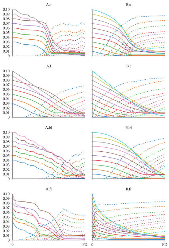
Figure 4.
Project configurations optimized (solid) and (dashed) curves.
While the latter is given by Equation (26),
As a result, a higher level of leads to a delay in materialization and a decrease in .
5. Discussion
This study aimed to develop a CMF to replace subjective decision-making in the depletion of CRs, considering project managers’ risk perceptions. This work developed the CMF and validated it on synthetic projects, representing eight extreme project configurations to be applied in any real project whose configuration falls between the eight tested.
The main results confirm the applicability of CMF in identifying combinations of , , and that drive contingency spending while minimizing concern for cost overruns. For a specific project, the CMF identifies three intervals. In the first interval, which ranges from zero to , the CR is statistically insufficient to address risks. Hence, delaying the use of the CR until a later stage of the project remains the only way to optimize its utilization. In the second interval, which ranges between and , the CMF examines the combinations of and to minimize the indicator. In the third interval, where , the CMF recommends mitigating any ST or LT cost overrun by setting since it is statistically unlikely for the project to exceed .
From a theoretical standpoint, the study provides several contributions. First, the CLD clarifies the relationships that connect project monitoring variables and the sequence of steps leading from the valuation of marginal work performed within a timeframe to estimating the variance between the project’s forecasted cost at completion and the available budget. Second, the CMF incorporates two indicators quantifying the concern for short- and long-term cost overruns (i.e., and ), the respective responses (i.e., and ), and thresholds ( and ). Third, the study offers a method to quantify the thresholds in a way that guides contingency spending, minimizing a project manager’s exposure to the risk of under or overestimating responses to cost overruns.
On a practical level, the CMF serves as a decision support tool to be implemented during PRM planning. Through simulation-optimized thresholds, the CMF determines the development of responses to cost overruns recorded during project execution, which in the simplest form consist of spending contingency reserves to acknowledge risk events, thus reducing the increase in that serves as the basis for project completion cost estimates. In this way, the CMF dictates the CR depletion strategy, replacing project managers’ risk attitudes and perceptions.
The study’s methodology relies on several key assumptions. Firstly, it assumes that CR is solely utilized to address cost overruns rather than proactively mitigating risks. This limitation may affect the method’s effectiveness when confronted with unforeseen risks, which are often difficult to anticipate and quantify. However, one can adjust the PDF for cost overruns to accommodate additional risks that can impact project activities. Secondly, the project execution simulation model assumes a uniform cost deviation PDF for all tasks. This assumption is unrealistic in real-world scenarios, where each task should have its PDF tailored to its specific characteristics, such as complexity, technology, and operational context. The choice of the PDF should be based on whether historical data are available to fit an empirical PDF or on information about the PDF mean, mode, and skewness. Lastly, the approach to calculating the adheres to EVM principles. While EVM offers simplicity and effectiveness for cost prediction, it may not adequately account for complex factors such as unknown risks. For example, the equation assumes that the remains constant until project completion, but it can fluctuate. Nonetheless, the CMF is insensitive to such assumptions, as it quantifies by setting .
6. Conclusions
CM is essential to project success, as it allows developing responses to keep project costs under control. This process consists of two steps: estimating the initial CR and using it based on the occurrence of cost overruns. The fundamental problem associated with CM is the high weight of the human factor in perceiving risks and developing responses. Managers make decisions based on their attitude and appetite, characterized by personal experience and external factors. Such subjectivity carries several risks related to the effectiveness of actions and the repercussions they may have on the project system.
Studies in the literature have addressed the problem of CM by focusing either on developing contingency depletion strategies, introducing thresholds to assess whether the project is in control, or analyzing the ripple effects between risk responses and project performance. This study proposes a CMF integrating all problems at once using the Monte Carlo approach. The whole RM process, including the CMF, can be summarized as follows:
- Identify project tasks;
- Identify risks impacting tasks;
- Estimate task cost distribution;
- (a)
- Define task cost point estimate;
- (b)
- Define estimating method, uncertainty drivers, and risks;
- (c)
- Anchor point estimate and adjust distribution;
- Define formula;
- Set CMF simulation parameters (i.e., , , , , , );
- Run CMF.
The CMF determines three intervals of initial CR based on the probability density function (PDF) of task cost deviation and their degree of correlation. The optimization algorithm then determines the thresholds for drawing on the CR in response to risk events that cause task cost overrun for each interval. Risk responses are developed based on matching two thresholds: one related to cost overruns in the ST and the other related to cost overruns in the LT. The project execution is simulated multiple times, changing the threshold levels. Given an initial CR level, the CMF optimizes the threshold levels to minimize the risk of cost overruns while ensuring the CR is used efficiently. This reduces the possibility that project managers develop suboptimal risk responses that could undermine a project’s cost and schedule performance. The CMF considers the statistical properties of task cost distributions and their correlation with other tasks, providing a more realistic approach to contingency management optimization. The ability to optimize the allocation of CRs based on statistical analysis and simulation can lead to better decision-making and cost control during project execution.
The proposed CMF integrates with standards and software related to project risk management. Concerning standards, the simulation model is consistent with the Monte Carlo simulation approaches described in project risk-specific standards including, but not limited to, ISO/IEC 62198 [55], ISO/IEC 31010 [56], PMI [1], and PMI [57]. Regarding software, the CMF can be coded from scratch (as in the case of this study), using either procedural or object-oriented programming, or developed using commercial software that allows for discrete-event modeling.
This study faced several limitations that warrant consideration. First, the study conceptualized the simulation model that represents project cost monitoring in a highly simplified manner. Specifically, time-related considerations are absent, whereas cost can be related to task duration and other cost drivers. Future studies can expand the model by incorporating additional variables impacting project execution and costs, such as schedule delay [58] or factors related to the external environment of the stakeholders’ organization [59]. Second, the study does not compare the proposed CMF with existing CMFs. Given the absence of standard CMFs and CMFs that specifically address concern for cost overruns in the short and long term, further research is needed to evaluate the proposed CMF’s relative strengths and weaknesses. Lastly, the study validates the CMF and the simulation model on synthetic projects, raising concerns about its effectiveness in real-world settings. The inability to simulate alternative decision paths and observe their outcomes in real projects limits the study’s ability to assess the CMF’s effectiveness. However, this is a hard limitation of all studies in project risk management proposing prescriptive methods. These assumptions highlight the need for further research to refine the CMF, compare it to established benchmarks, and validate its effectiveness in real-world project environments.
Author Contributions
Conceptualization, F.M.O., A.D.M. and C.R.; methodology, F.M.O.; software, F.M.O.; validation, F.M.O.; formal analysis, F.M.O.; investigation, F.M.O.; resources, F.M.O.; data curation, F.M.O.; writing—original draft preparation, F.M.O. and G.C.; writing—review and editing, F.M.O., A.D.M. and G.C:; visualization, F.M.O.; supervision, A.D.M. and C.R.; project administration, F.M.O. All authors have read and agreed to the published version of the manuscript.
Funding
This research received no external funding.
Data Availability Statement
Dataset available on request from the authors.
Conflicts of Interest
The authors declare no conflicts of interest.
Abbreviations
The following abbreviations are used in this manuscript:
| CDF | Cumulative density function |
| CLD | Causal loop diagram |
| CLT | Central limit theorem |
| CM | Contingency management |
| CMF | Contingency management framework |
| CR | Contingency reserve |
| EVM | Earned value management |
| ES | Earned schedule |
| iid | Independent and identically distributed |
| LT | Long term |
| MC | Monte Carlo (method) |
| PERT | Program evaluation review technique |
| Probability density function | |
| PRM | Project risk management |
| ST | Short term |
References
- PMI. The Standard for Risk Management in Portfolios, Programs, and Projects; Project Management Institute, Inc.: Newton Square, PA, USA, 2019; p. 194. [Google Scholar]
- Chapman, R.J. Complexity Theory and System Dynamics for Project Risk Management. In Decision Management: Concepts, Methodologies, Tools, and Applications; IGI Global: Hershey, PA, USA, 2017; Volume 1–4, pp. 401–425. [Google Scholar] [CrossRef]
- Olawale, Y.A.; Sun, M. Cost and time control of construction projects: Inhibiting factors and mitigating measures in practice. Constr. Manag. Econ. 2010, 28, 509–526. [Google Scholar] [CrossRef]
- Liu, J.; Zhao, X.; Yan, P. Risk Paths in International Construction Projects: Case Study from Chinese Contractors. J. Constr. Eng. Manag. 2016, 142, 05016002. [Google Scholar] [CrossRef]
- Gharaibeh, H.M. Cost Control in Mega Projects Using the Delphi Method. J. Manag. Eng. 2014, 30, 04014024. [Google Scholar] [CrossRef]
- PMI. A Guide to the Project Management Body of Knowledge, 6th ed.; Project Management Institute: Newton Square, PA, USA, 2017. [Google Scholar]
- Dikmen, I.; Budayan, C.; Talat Birgonul, M.; Hayat, E. Effects of Risk Attitude and Controllability Assumption on Risk Ratings: Observational Study on International Construction Project Risk Assessment. J. Manag. Eng. 2018, 34, 04018037. [Google Scholar] [CrossRef]
- Chekah, A.; NedaYeganli; Yakchali, S.H. Organizational Behavior Factors In Responding To Project Risks Using System Dynamics Approach. In Proceedings of the ICCPM 2011—Construction and Project Management, Singapore, 16–18 September 2011; Volume 15, pp. 84–88. [Google Scholar]
- Haji-Kazemi, S.; Andersen, B.; Krane, H.P. A review on possible approaches for detecting early warning signs in projects. Proj. Manag. J. 2013, 44, 55–69. [Google Scholar] [CrossRef]
- Kristinsdottir, A. Risks and decision making in development of new power plant projects. Diss. Abstr. Int. Sect. D Humanit. Soc. Sci. 2013, 74, No–Specified. [Google Scholar]
- Hartono, B. From project risk to complexity analysis: A systematic classification. Int. J. Manag. Proj. Bus. 2018, 11, 734–760. [Google Scholar] [CrossRef]
- Xie, H.; AbouRizk, S.; Zou, J. Quantitative Method for Updating Cost Contingency throughout Project Execution. J. Constr. Eng. Manag. 2012, 138, 759–766. [Google Scholar] [CrossRef]
- Damnjanovic, I.; Reinschmidt, K. Data Analytics for Engineering and Construction Project Risk Management. In Risk, Systems and Decisions; Springer International Publishing: Cham, Switzerland, 2020. [Google Scholar] [CrossRef]
- Ford, D.N. Achieving Multiple Project Objectives through Contingency Management. J. Constr. Eng. Manag. 2002, 128, 30–39. [Google Scholar] [CrossRef]
- Barraza, G.A.; Bueno, R.A. Cost Contingency Management. J. Manag. Eng. 2007, 23, 140–146. [Google Scholar] [CrossRef]
- Moselhi, O.; Salah, A. Fuzzy Set-Based Contingency Estimating and Management. In Proceedings of the ISARC 2012—29th International Symposium of Automation and Robotics in Construction, Eindhoven, The Netherlands, 26–29 June 2012. [Google Scholar] [CrossRef]
- Salah, A.; Moselhi, O. Contingency modelling for construction projects using fuzzy-set theory. Eng. Constr. Archit. Manag. 2015, 22, 214–241. [Google Scholar] [CrossRef]
- Eldosouky, I.A.; Ibrahim, A.H.; Mohammed, H.E.D. Management of construction cost contingency covering upside and downside risks. Alex. Eng. J. 2014, 53, 863–881. [Google Scholar] [CrossRef]
- Hammad, M.W.; Abbasi, A.; Ryan, M.J. A new method of cost contingency management. In Proceedings of the 2015 IEEE International Conference on Industrial Engineering and Engineering Management (IEEM), Singapore, 6–9 December 2015; pp. 38–42. [Google Scholar] [CrossRef]
- Hammad, M.W.; Abbasi, A.; Ryan, M.J. Allocation and Management of Cost Contingency in Projects. J. Manag. Eng. 2016, 32, 04016014. [Google Scholar] [CrossRef]
- Traynor, B.A.; Mahmoodian, M. Time and cost contingency management using Monte Carlo simulation. Aust. J. Civ. Eng. 2019, 17, 11–18. [Google Scholar] [CrossRef]
- Kim, S.G.; Kim, J.J.; Kim, K.R. A Risk Threshold Calculation Methodology for the Construction Projects Applying Value at Risk. In Proceedings of the Construction Research Congress 2005, San Diego, CA, USA, 5–7 April 2005; pp. 1–9. [Google Scholar] [CrossRef]
- Pajares, J.; López-Paredes, A. An extension of the EVM analysis for project monitoring: The Cost Control Index and the Schedule Control Index. Int. J. Proj. Manag. 2011, 29, 615–621. [Google Scholar] [CrossRef]
- Colin, J.; Vanhoucke, M. Setting tolerance limits for statistical project control using earned value management. Omega 2014, 49, 107–122. [Google Scholar] [CrossRef]
- Colin, J.; Martens, A.; Vanhoucke, M.; Wauters, M. A multivariate approach for top-down project control using earned value management. Decis. Support Syst. 2015, 79, 65–76. [Google Scholar] [CrossRef]
- Kim, B.C. Dynamic Control Thresholds for Consistent Earned Value Analysis and Reliable Early Warning. J. Manag. Eng. 2015, 31, 04014077. [Google Scholar] [CrossRef]
- Ballesteros-Pérez, P.; Sanz-Ablanedo, E.; Mora-Melià, D.; González-Cruz, M.C.; Fuentes-Bargues, J.L.; Pellicer, E. Earned Schedule min-max: Two new EVM metrics for monitoring and controlling projects. Autom. Constr. 2019, 103, 279–290. [Google Scholar] [CrossRef]
- Kim, B.C.; Pinto, J.K. What CPI = 0.85 Really Means: A Probabilistic Extension of the Estimate at Completion. J. Manag. Eng. 2019, 35, 04018059. [Google Scholar] [CrossRef]
- Chen, Z.; Demeulemeester, E.; Bai, S.; Guo, Y. A Bayesian approach to set the tolerance limits for a statistical project control method. Int. J. Prod. Res. 2020, 58, 3150–3163. [Google Scholar] [CrossRef]
- Rodrigues, A.G. Managing and Modelling Project Risk Dynamics A System Dynamics-based Framework. In Proceedings of the Fourth European Project Management Conference: PMI Europe, London, UK, 6–7 June 2001; Volume 7, pp. 6–7. [Google Scholar]
- Chritamara, S.; Ogunlana, S.O.; Bach, N.L. System dynamics modeling of design and build construction projects. Constr. Innov. 2002, 2, 269–295. [Google Scholar] [CrossRef]
- Wang, Q.f.; Ning, X.q.; You, J. Advantages of System Dynamics Approach in Managing Project Risk Dynamics. J. Fudan Univ. Nat. Sci. 2005, 44, 201–206. [Google Scholar]
- Howick, S.; Ackermann, F.; Eden, C.; Williams, T. Understanding the causes and consequences of disruption and delay in complex projects: How system dynamics can help. In Encyclopedia of Complexity and Systems Science; Springer: Berlin/Heidelberg, Germany, 2009; pp. 1–33. [Google Scholar]
- Ding, R.; Gao, S.; Wang, L.; Sun, T. Network dynamic analysis based risk management for collaborative innovation projects. In Proceedings of the 12th International Scientific and Technical Conference on Computer Sciences and Information Technologies, CSIT 2017, Lviv, Ukraine, 5–8 September 2017; Volume 2, pp. 140–144. [Google Scholar] [CrossRef]
- Wang, J.; Yuan, H. System Dynamics Approach for Investigating the Risk Effects on Schedule Delay in Infrastructure Projects. J. Manag. Eng. 2017, 33, 04016029. [Google Scholar] [CrossRef]
- Leon, H.; Osman, H.; Georgy, M.; Elsaid, M. System Dynamics Approach for Forecasting Performance of Construction Projects. J. Manag. Eng. 2018, 34, 04017049. [Google Scholar] [CrossRef]
- Cunbin, L.; Yunqi, L.; Shuke, L. Human resources risk element transmission model of construction project based on system dynamic. Open Cybern. Syst. J. 2015, 9, 295–305. [Google Scholar] [CrossRef]
- Zhang, M.; Wang, X.; Mannan, M.S.; Qian, C.; Wang, J. A system dynamics model for risk perception of lay people in communication regarding risk of chemical incident. J. Loss Prev. Process Ind. 2017, 50, 101–111. [Google Scholar] [CrossRef]
- Leite, L.d.S.; de Farias Neto, A.R.; de Lima, F.L.; Chaim, R.M. Analyzing and Modeling Critical Risks in Software Development Projects: A Study Based on RFMEA and Systems Dynamics. Proc. Adv. Intell. Syst. Comput. 2021, 1368, 22–35. [Google Scholar] [CrossRef]
- De Marco, A.; Rafele, C.; Thaheem, M.J. Dynamic Management of Risk Contingency in Complex Design-Build Projects. J. Constr. Eng. Manag. 2016, 142, 04015080. [Google Scholar] [CrossRef]
- De Marco, A.; Narbaev, T.; Ottaviani, F.M.; Vanhoucke, M. Influence of cost contingency management on project estimates at completion. Int. J. Constr. Manag. 2023, 0, 1–11. [Google Scholar] [CrossRef]
- Ayub, B.; Thaheem, M.J.; Ullah, F. Contingency Release During Project Execution: The Contractor’s Decision-Making Dilemma. Proj. Manag. J. 2019, 50, 734–748. [Google Scholar] [CrossRef]
- ISO 31000:2018; Risk Management. International Organization for Standardization: Geneva, Switzerland, 2018.
- Moeller, R.R. Executive’s Guide to Coso Internal Controls: Understanding and Implementing the New Framework; John Wiley & Sons: Hoboken, NJ, USA, 2013. [Google Scholar]
- Dalli Gonzi, R.; Grima, S.; Kizilkaya, M.; Spiteri, J. The DALI Model in Risk-Management Practice: The Case of Financial Services Firms. J. Risk Financ. Manag. 2019, 12, 169. [Google Scholar] [CrossRef]
- Kruf, J.P.; Grima, S.; Kizilkaya, M.; Spiteri, J.V.; Slob, W.; O’Dea, J. The PRIMO FORTE Framework for Good Governance in Public, Private and Civic Organisations: An Analysis on Small EU States. Eur. Res. Stud. J. 2019, XXII, 15–34. [Google Scholar]
- Law, A. How to conduct a successful simulation study. In Proceedings of the 2003 Winter Simulation Conference, New Orleans, LA, USA, 7–10 December 2003; pp. 66–70. [Google Scholar] [CrossRef]
- Banks, J.; Carson, J.; Nelson, B.; Nicol, D. Discrete-Event System Simulation, 5th ed.; Prentice-Hall: Saddle River, NJ, USA, 2009; p. 648. [Google Scholar]
- Lance Stephenson, H. AACE International Total Cost Management Framework: An Integrated Approach to Portfolio, Program, and Project Management; AACE International: Morgantown, WV, USA, 2015; p. 332. [Google Scholar]
- Warburton, R.D.; Ottaviani, F.M.; De Marco, A. Critical Analysis of Linear and Nonlinear Project Duration Forecasting Methods. J. Mod. Proj. Manag. 2023, 11, 186–199. [Google Scholar]
- Du, J.; Kim, B.C.; Zhao, D. Cost Performance as a Stochastic Process: EAC Projection by Markov Chain Simulation. J. Constr. Eng. Manag. 2016, 142, 04016009. [Google Scholar] [CrossRef]
- Vose, D. Risk Analysis: A Quantitative Guide, 3rd ed.; John Wiley & Sons: Hoboken, NJ, USA, 2008; p. 735. [Google Scholar]
- PMI. Practice Standard for Earned Value Management, 2nd ed.; Project Management Institute: Newton Square, PA, USA, 2005; p. 135. [Google Scholar]
- Everitt, B.S.; Skrondal, A. The Cambridge Dictionary of Statistics; Cambridge University Press: Cambridge, UK, 2010. [Google Scholar] [CrossRef]
- EN 62198-2014; Managing Risk in Projects — Application Guidelines. International Organization for Standardization (ISO) and International Electrotechnical Commission (IEC): Geneva, Switzerland, 2014.
- EN IEC31010-2019; Risk Management — Risk Assessment Techniques. Standard, International Organization for Standardization (ISO) and International Electrotechnical Commission (IEC): Geneva, Switzerland, 2019.
- PMI. Practice Standard for Project Risk Management; Project Management Institute, Inc.: Newton Square, PA, USA, 2009; p. 128. [Google Scholar]
- Derakhshanfar, H.; Ochoa, J.J.; Kirytopoulos, K.; Mayer, W.; Langston, C. A cartography of delay risks in the Australian construction industry: Impact, correlations and timing. Eng. Constr. Archit. Manag. 2021, 28, 1952–1978. [Google Scholar] [CrossRef]
- Khodeir, L.M.; Nabawy, M. Identifying key risks in infrastructure projects—Case study of Cairo Festival City project in Egypt. Ain Shams Eng. J. 2019, 10, 613–621. [Google Scholar] [CrossRef]


Disclaimer/Publisher’s Note: The statements, opinions and data contained in all publications are solely those of the individual author(s) and contributor(s) and not of MDPI and/or the editor(s). MDPI and/or the editor(s) disclaim responsibility for any injury to people or property resulting from any ideas, methods, instructions or products referred to in the content. |
© 2024 by the authors. Licensee MDPI, Basel, Switzerland. This article is an open access article distributed under the terms and conditions of the Creative Commons Attribution (CC BY) license (https://creativecommons.org/licenses/by/4.0/).