NEMAS: Norm Entrepreneurship in Multi-Agent Systems ^†

Abstract

We propose a framework that integrates norm entrepreneurship from human society into the dynamics of an agent society. Most work in agent coordination in a distributed environment studies norms that are provided to agents as part of their specification or distributed from centralised agents. Exploring an alternate perspective, we focus on peer-to-peer interaction by providing the agents with the freedom to initiate norm creation in demanding situations like a potential interference. This paper explores the concept of norm entrepreneurship through proactive establishment and emergence of norms by agents. A common approach in prior work focuses on coordination problems that are reduced to simple game theory models involving the simultaneous performance of a single action by each agent. Instead, we define the concept of a local coordination plan (LCP), which is a sequence of actions from each agent to cope with an interference in their normal course of action. We identify LCPs across various scenarios and abstract these plans using coordination state machines (CSMs). A coordination state machine contains a separate state machine for each agent where the states encapsulate the potentially constrained and suboptimal movement options agents have at a given time. We also explore how multiple LCPs lead to a coordination state machine of the same format and how a coordination state machine can abstract across multiple scenarios.

1. Introduction

Consider the etiquette that we tend to follow on our daily commute. On sidewalks, we are mindful not to jostle past others. While walking with someone, we go single file on a crowded walkway. While listening to a personal collection of podcasts in a train, we make sure to use earbuds rather than speakers. Of many such codes of conduct that we follow in a community, some are unwritten expected forms of behaviours, while others became formally codified to become legally enforceable. Social norms, which are the unwritten rules of conduct, help to maintain order and predictability in a society. They offer standards on behaviours that are considered acceptable or unacceptable among the members in a social group and provide a mechanism that people use to coordinate with each other in society.

So, how do norms emerge in a community? More than 100 years have passed since Sumner [1] wrote a treatise on “Folkways” and “Mores”, which are unwritten rules that are expected to be followed in a community. Sumner states that:

“The folkways are habits of the individual and customs of the society which arise from efforts to satisfy needs. The step an individual takes for an immediate motive is repeated when similar situations arise. This repetition of certain acts produces a habit in the individual. As this habit becomes widely acceptable in a society, people tend to comply with them even though they are not enforced by any authority and it thus evolves as a norm in the group.”

We might presume that behind such norms in a group, there is an entrepreneurial mindset. We propose to borrow and adapt this entrepreneurial mindset from human society to multi-agent systems, where agents interact in a shared environment to achieve individual or common goals. One noteworthy strand of work on norms in social groups by various disciplines like anthropology, social science, economics, etc. is regarding “norm entrepreneurs”1 and their impact on society. A norm entrepreneur (NE) is broadly considered as a person interested in changing social norms or as lawmakers or government agencies who could influence the dynamics of norm-following behaviours in a society. Finnemore and Sikkink [4] state that many international norms began as domestic norms and become international through the efforts of entrepreneurs of various kinds, which indicates how entrepreneurs become carriers of a norm and influence the society to follow them.

Our work proposes to adopt this concept of norm entrepreneur to a multi-agent system. We introduce a framework in a decentralised multi-agent environment where any agent is at liberty to be a norm entrepreneur and propose solutions to any potential interference they come across while acting in the environment [5]. Over a period of time, the coordinating solutions they propose may emerge as norms in the society. Our focus is on a peer-to-peer, bottom-up approach like folkways [1], where ideas to solve a problem emerge from an individual and later evolve to become norms.

This paper extends the PAAMS’23 paper titled “Towards Norm Entrepreneurship in Agent societies” [5]. The earlier version of the paper focused on how the norm entrepreneur agent identifies a potential interference and generates Pareto-optimal solutions to the interference, considering individual and combined regret compared to the agents’ individual optimal plans. The paper also introduced the concept of “regret landscapes”, which depict coordination problem in terms of potential agent regret. The extended version of our work in this article presents the next phase of abstraction. We present the notion of a coordination state machine (CSM) to encapsulate the solutions devised by the entrepreneurial agent. We discuss how these abstracted state machine can be reused for different environments (unlike LCPs). The CSM will provide clear instructions on what actions an agent must refrain from or must undertake as part of the solution, highlighting that coordination is a social agreement with a regret.

The remainder of the paper is structured as follows: Section 1.1 and Section 1.2 discuss the background and motivation for our study. Section 2 outlines the problem formally, presents our proposed framework, and provides our solution and examples. Section 3 discusses the results obtained. Finally, Section 4 summarises the contributions of this work.

1.1. Background and Motivation

Sociologists say that norms emerge in a society as a result of two factors: (i) as a result of unintended consequences of human action, and (ii) by human design. According to Opp [6], norms are mostly an unintended result of uncoordinated human interaction, i.e., norms may emerge spontaneously like many customs of everyday life. To illustrate this approach, he analyses an example of how an unplanned non-smoking norm emerges in a society. Writing about norm emergence by human design, he refers to the norms created intentionally like laws, contracts between businesses, and the like. Centola and Baronchelli [7] present experimental results that show how social conventions emerge spontaneously. This work is inspired by their statement that social conventions emerge as consequences of individual efforts to coordinate locally with one another.

1.2. Research Gap

Boella et al. [8] define a normative multi-agent system as follows:

“… a multi agent system together with normative systems in which agents on the one hand can decide whether to follow the explicitly represented norms, and on the other the normative systems specify how and in which extent the agents can modify the norms.”

In most of the existing literature on normative multi-agent systems, norms are provided to agents as part of their specification, created in a normative system through a norm synthesis process or learned from observation and experience. Norm synthesis requires a governing mechanism or a special centralised agent to generate and distribute the norms. Some noteworthy studies along this strand are the approaches of Shoham and Tennenholtz [9], Morales et al. [10,11,12,13], Alechina et al. [14], and Riad and Golpayegani [15,16,17]. These works commonly model the coordination problem as a simultaneous matrix game, as illustrated in Figure 1 [10]. In this approach, norms are modelled as a single joint action that is obligatory or prohibited. The agent-directed norm synthesis proposed by Morris-Martin et al. [18,19,20] decentralises the norm synthesis across a team of specialist synthesiser agents, each serving a community of agents. An agent can contact its synthesiser agent to initiate the process, and a consensus across all synthesiser agents must be reached (possibly with a final approval from an oracle agent) for a new norm or a norm modification to be adopted. Thus, the single central norm synthesiser in prior approaches is replaced by a group of empowered agents. There will be many MAS applications for which this is not feasible or desirable, especially when the agents are peers with no hierarchy in place. Also, coordination is often more complicated than the work on norm synthesis.

Consider a park where agents (A and B) move around with the intention of reaching their desired locations. Agents are expected to stay on the pathway and avoid walking through natural areas like the lawn. In this work, we consider agents that are not part of a team and are moving amongst potentially many unknown agents. Hence, they do not consider the presence of other agents until they reach any potential interference. In our model, the park is represented as a grid (Figure 2) and it includes features that require agents to handle potential interference along their way. The features in Figure 2 are represented by the following colours:

• Green cells: lawn;
• Brown cells: pathway;
• Grey cells: open space.

Out of many potential interference layouts used in our experiments, for now, we consider four coordination patterns to express our idea: the ’parallel path pattern’, the ’extended parallel path pattern’, the ’common goal pattern’, and the ’zigzag pattern’ (Figure 2). Here, A and B indicate the current locations of the two agents, and $G_a$ and $G_b$ show their goal locations.

Initially the agents generate individual optimal policies to reach their goals. As the agents come across a potential interference, one of these agents may have to wait until the other exits a pathway, or it will have to expend extra time in using an alternative pathway. Otherwise, they may block each other’s progress until one backs off. Instead of attempting to avoid other agents as part of the initial planning process, we consider what strategies agents can employ to address each inter-agent interaction that agents may encounter while navigating their environment and how agents can attain coordination without the need of a central authority.

2. Materials and Methods

We approach the problem through a five-stage process as outlined in the framework (Figure 3). Section 2.1.1 to  Section 2.1.5 elaborate on these stages.

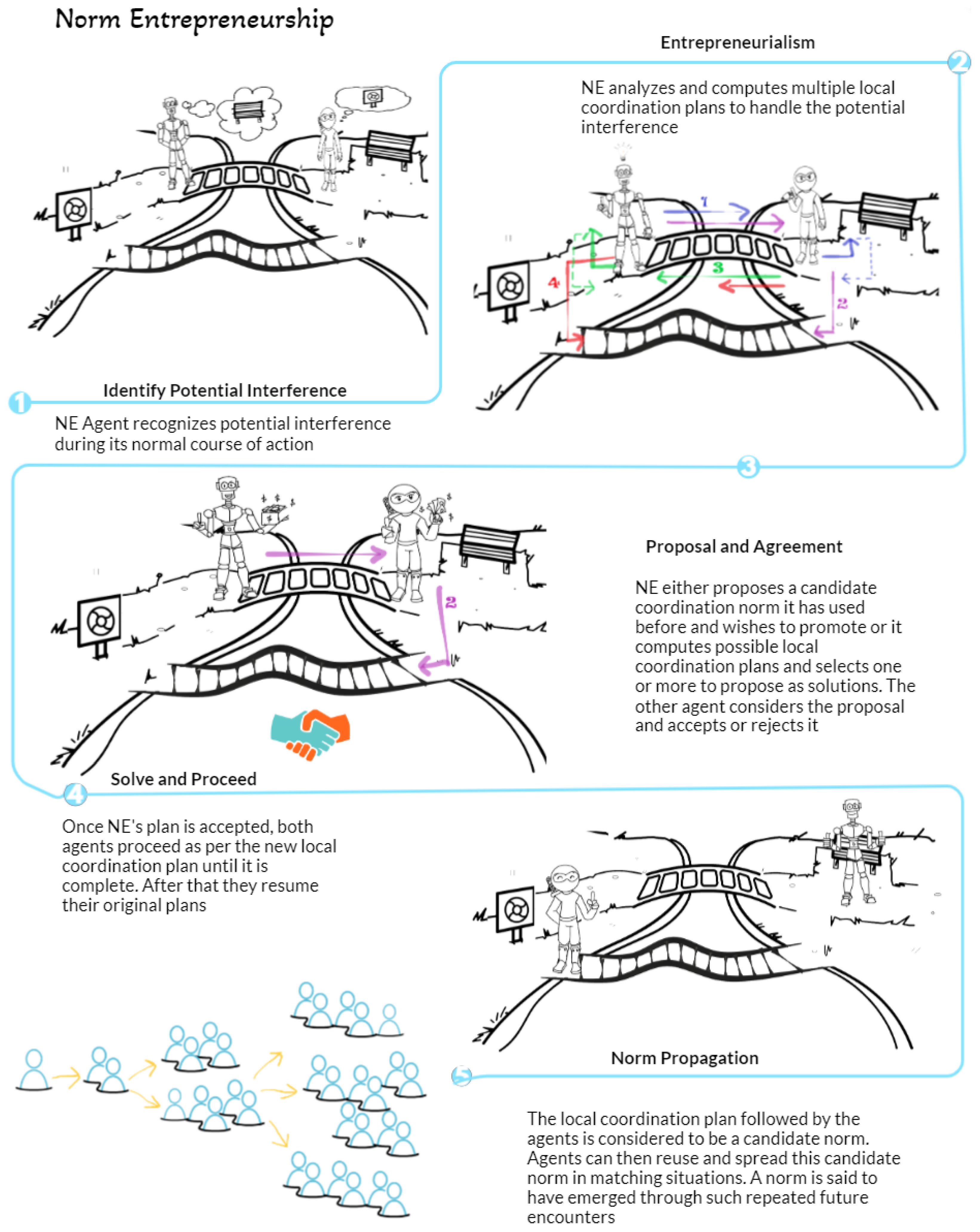
2.1. The Five Stages of Our Norm Entrepreneurship Framework

2.1.1. Identifying Potential Interference

Agents move through the environment following their optimal policies until they reach a potential interference. A potential interference is detected when another agent is observed within a certain distance and it appears to be entering a potentially contested region. Once a norm entrepreneur agent recognises a potential interference, the agent generates a region of coordination (ROC), infers2 an approximate goal location for the other agent within the ROC and then generates possible local coordination plans.

To enhance comprehension, we first focus on a single pattern (Figure 4) to explain the model. Further elaboration on other patterns can be found in Section 2.6. In Figure 4, agent A identifies a potential interference as soon as A and B reach opposite sides of the lawn. Agent A then proceeds with entrepreneurship.

2.1.2. Local Coordination Planning by Entrepreneurs

The crux of our framework is depicted in Figure 3. Existing studies propose the following mechanisms to avoid or handle interference in a multi-agent system: design a collision free environment, provide a mechanism for collision avoidance, or re-plan an agent’s course of action when it confronts a collision. However, all these approaches restrict the agent’s mobility by avoiding a potential collision in advance as opposed to the real world scenario whereas humans devise strategies to handle such situations as and when they occur. Our approach of generating a local coordination plan addresses this research gap. Once an agent starts to move along the optimal path, it will recognise situations where other agents might hamper its course of action. As two or more3 agents come across such interference, a norm entrepreneur may propose a coordination plan to handle the hindrance locally, within the ROC.

The proposal of a local coordination plan has two cases. The first is where the norm entrepreneur agent computes a new local coordination plan, abstracted into a coordination state machine (CSM) explained in Section 2.5. In the second case, a previously used coordination state machine that matches the current situation may be proposed for reuse.

2.1.3. Proposal and Agreement

The norm entrepreneur (NE) agent either proposes a candidate coordination norm it has used before and wishes to promote or it computes possible local coordination plans and selects one or more to propose as solutions using the abstracted coordination state machine notation described in Section 2.5. The other agent considers the proposal and has the choice to accept or reject. In Figure 3, we can see that the NE agent has proposed the local coordination plan numbered 2. If the other agent accepts the proposal, it will take the alternative pathway to cross and reach its destination, thereby deviating from its original plan. The entrepreneur is required to choose either (a) a single CSM that has equal regret (the extra cost of following the coordination plan, compared to the optimal plan) for the two agents and also has the least total regret, or if that does not exist, then (b) two sets of CSMs: one containing CSMs with a lower regret for one agent and another containing CSMs with lower regret for the other agent. Presenting only one CSM implies this is the case. The other agent can agree or disagree. If it disagrees, then it is clearly not interested in coordinating so the negotiation ends and both agents follow their individual optimal plans. In case (b), in situations where multiple CSMs exist, each agent can opt for the most favourable plan from their respective set of options. After both agents have made their choices, a distributed coin toss [22] can be used to decide the ultimate selection between them. This is a protocol allowing two or more parties to jointly generate a random value in the absence of trust between them, with neither agent able to significantly influence the outcome. A distributed coin toss promotes fairness in an environment where agents need to agree on outcomes without relying on a central authority. Additionally, in order to ensure that the norm entrepreneur agent is not cherry picking the proposed CSMs, auditor agents can be employed in the environment. The encounters with entrepreneurs could be recorded to be provided later to auditors. Alternatively, there could be undercover inspectors in the environment.

2.1.4. Plan Execution

Once a coordination state machine is accepted, both the agents proceed with this CSM until it is executed completely and the agents exit the region of coordination4. They then resume their optimal policy. When a CSM has been successfully used, the norm entrepreneur can further abstract it so it can match a wider range of scenarios and in later encounters a further more general version may be promoted by the NE.

2.1.5. Norm Propagation

According to Savarimuthu and Cranefield [23], from a societal viewpoint, the important stages of the norm lifecycle are the formation stage, the propagation stage, and the emergence stage. The norm formation stage considers how agents can create norms in a society and how they can identify the norms that have been created. The norm propagation stage is where norms are spread and enforced in the society. The emergence stage is characterised by determining the extent of the spread of a norm in the society. Since norms are considered as behavioural regularities that guide agents’ decisions in a social environment [24], we address the question of how a local coordination plan proposed by a norm entrepreneur agent could emerge as a norm.

We consider that once a coordination proposal is accepted by another agent during the proposal and agreement stage, it then becomes a candidate coordination norm for situations that it applies to. Agents can reuse and spread this candidate norm through the society in similar situations that may arise later during their travels. The norm emerges through repeated future encounters with agents who will promote these norms. For example, a norm could take the following form: in a situation matching pattern X, an agent must conform to its role in CSM Y.

A norm is said to have emerged when a candidate norm is accepted by a high proportion of agents. Once the norm has emerged, agents do not need to compute solutions in interference situations similar to those they might come across at a later stage. Instead, they could just execute the norms that have emerged already. The emergence of a norm depends on a coordination plan being abstracted sufficiently to apply to multiple situations that involve similar coordination problems. Additional conditions may be proposed by the norm entrepreneur to share the coordination costs on average, e.g., that an agent travelling towards certain focal points should incur the greater regret of coordination.

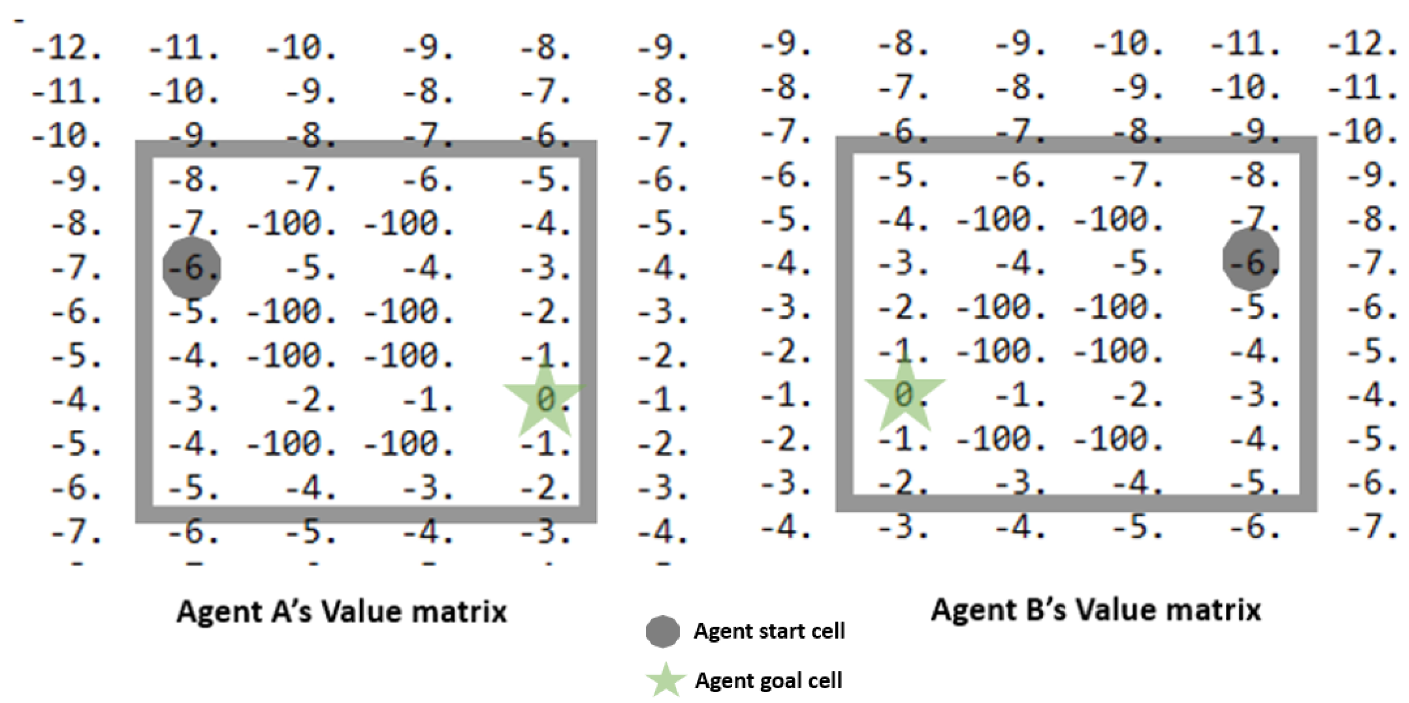
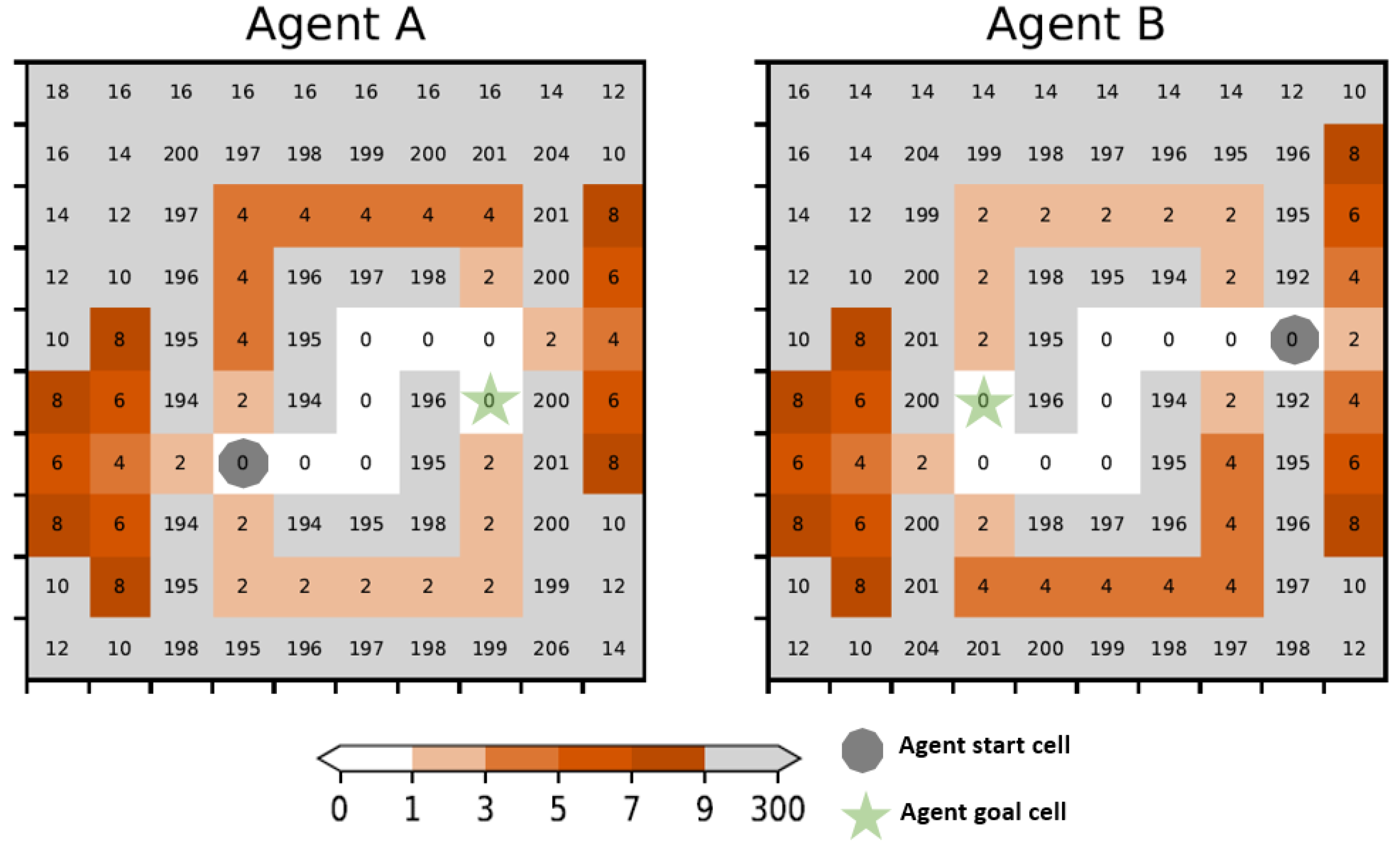
2.2. Individual Agent Planning

We model each agent a as a Markov decision process. The model is defined by a six-tuple $(S,A,T_a,R_a,\gamma ,g_a)$, where

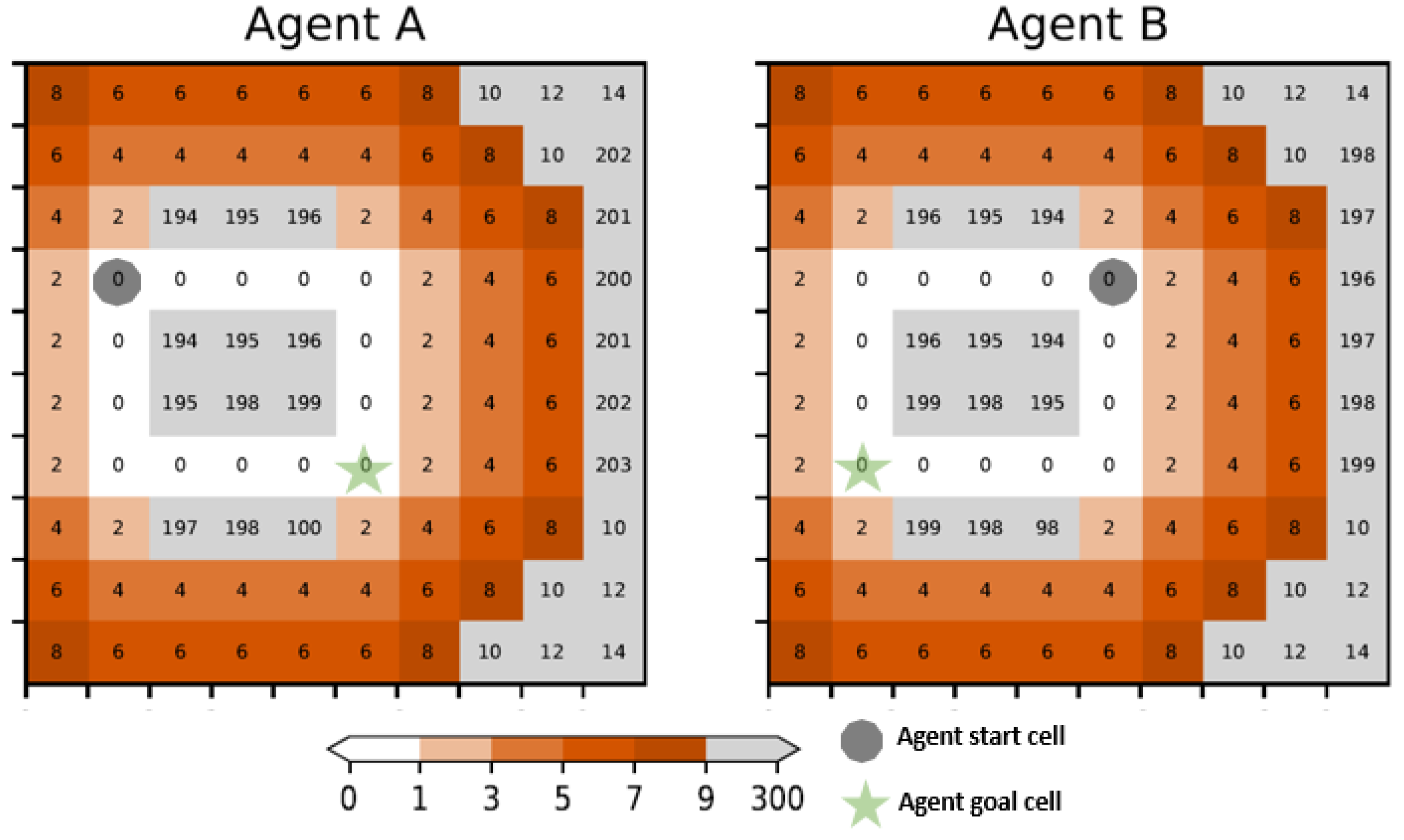
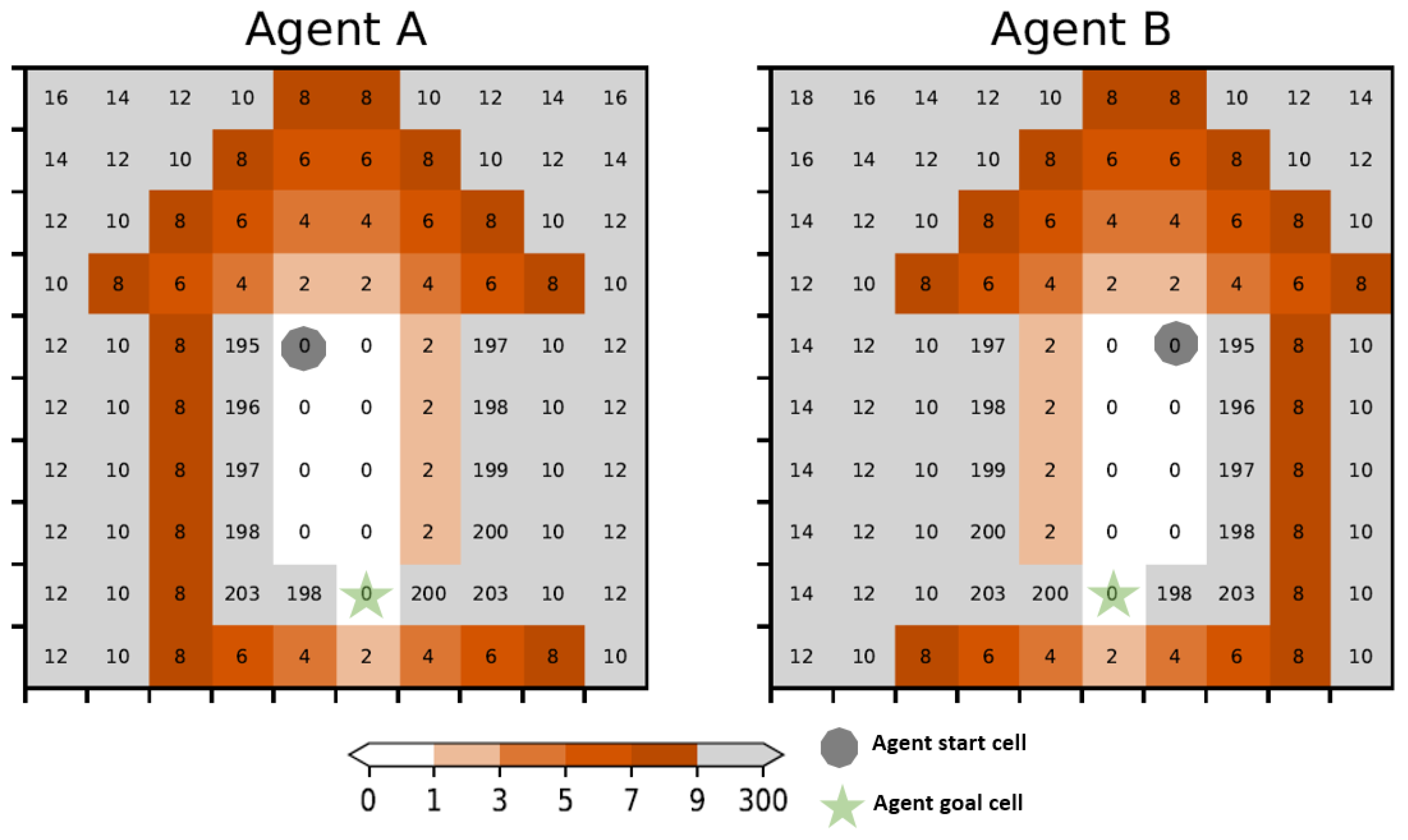
• S is the finite set of states. In this paper, the states are cells in a grid environment such as those shown in Figure 2;
• A is the finite set of possible actions that can be taken at each state;
• $T_a(s,\alpha ,s^{\prime })$ represents the probability of transitioning from one state to another given a particular action;
• $R_a(s,\alpha ,s^{\prime })$ is a function that returns the reward that an agent receives after taking action $\alpha$ in state s resulting in state $s^{\prime }$;
• $\gamma$ is the discount factor, a value between 0 and 1 that represents the preference for immediate rewards over future rewards. We set $\gamma$ to 1 as we consider finite horizon planning problems;
• $g_a$ is the goal state.

S and A are the same for each agent.

We use an absorbing state model, in which the goal state only has a zero-reward transition to itself and all other transitions have a negative reward representing the cost of movement. Also, $T_a$ and $R_a$ only differ between the agents due to their different absorbing states $g_a$.

Agents use their own local planning procedure to generate a policy to reach their respective goal without considering other agents. Each agent performs probabilistic planning using the value iteration algorithm [25] to produce a value $V_a^g\left(C\right)$, specific to that agent (a), for each cell c in the grid. This is the expected cumulative reward of following an optimal path from that cell to the goal. These values are used to produce an optimal policy that defines for each cell a probability distribution governing the choice of actions to be performed when in that state.

For each state $s\in S$, the value function $V_a\left(s\right)$ is:

$$V_a^g\left(s\right)\leftarrow \underset{\alpha \in A}{max}\sum _{s^{\prime }\in S}{T}_a(s,\alpha ,s^{\prime })·[R_a(s,\alpha ,s^{\prime })+\gamma ·V_a^g\left(s^{\prime }\right)]$$

The figure on the left of Figure 5 illustrates the values assigned to each cell for agent A, while the right side illustrates those for agent B. The circle represents the start cells and the thin-edged stars represent the goals.

2.3. Coordination Planning by Entrepreneurs

In Figure 3, we can see multiple local coordination plans that are numbered, which the NE agent has computed as the first step to solve the potential interference. The agent does this by executing a heuristic search over a space of joint actions in the region of coordination (ROC). The square in Figure 5 represents an ROC. A multi-objective heuristic search is carried out in the defined ROC. We adapted the NAMOA* algorithm for the multi-objective heuristic graph search [26]. The objectives we consider are the regret of each agent separately and their total regret, where an agent’s regret is its extra cost of reaching the goal when following the coordinate plan instead of its optimal policy. NAMOA* generates multiple plans that are Pareto-optimal solutions to the local planning problem, i.e., each plan has an associated vector of values, one for each objective, and only non-dominated plans are returned.

Consider Figure 4. If, for brevity, we consider only local coordination plans that are optimal for A, in the parallel path pattern, A can follow an optimal path to cross the park, while B chooses its alternative optimal path. In this scenario, both agents are operating optimally despite agent B opting for a different path. However, there could be instances where coordination planning leads one or both agents to take suboptimal paths individually (for example, in the zigzag pattern in Figure 2, an agent opting for the alternate route must proceed suboptimally).

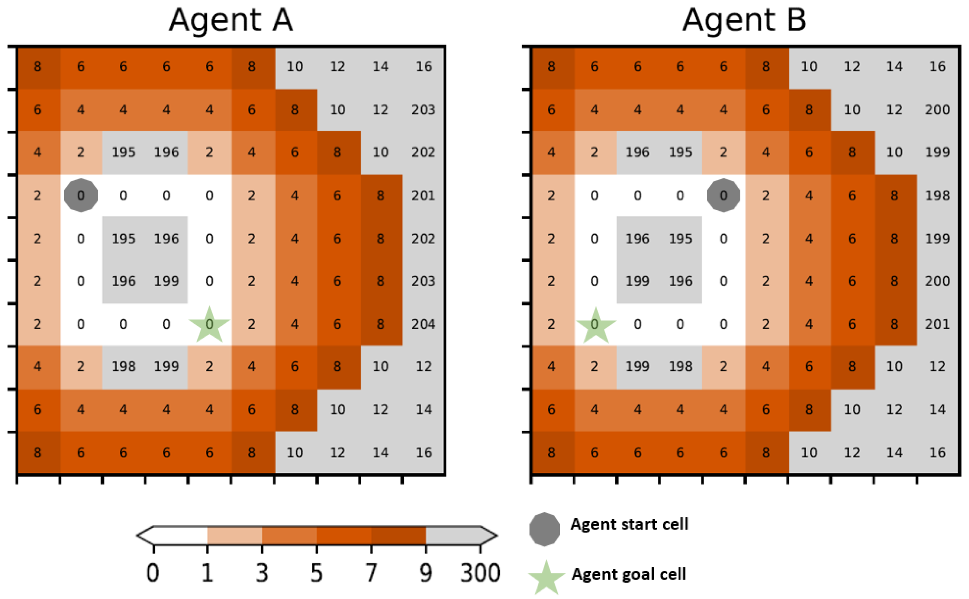
2.4. Regret Landscapes

According to decision theory, regret is a numeric measure of the difference between a choice made and the optimal choice. When a norm entrepreneur agent identifies a potential interference, it computes a solution to resolve the interference. This solution might have a suboptimal plan being offered to either or both of the agents. Hence, there is regret compared to the hypothetical case of following the optimal plan unimpeded.

To characterise the effect of the environment on the agent coordination problem, we define regret landscapes that show the regret that an agent must bear when required to deviate from its optimal path. From its initial individual planning, an agent knows its valuation for all the cells in the region of coordination, and has an optimal path between its start (s) and goal (g) positions within that region. It can also calculate the shortest path from s to each other cell in the region. Suppose the agent finds itself at some cell c that it reached while following an LCP. We define the regret that it would have from having to detour through c rather than following its optimal path. The regret landscapes are calculated without reference to any specific LCP, so we make the assumption that c was reached optimally from s.

The regret $R_a^{s,g}\left(c\right)$ is defined as follows:

$$R_a^{s,g}\left(c\right)=(sp{c}_a(s,c)+V_a^g\left(c\right))-sp{c}_a(s,g)$$

where $sp{c}_a(s,c)$ denotes the shortest path cost from the start location s to cell c;

Figure 6 shows the regret landscapes of agents A and B for the parallel path pattern. The higher the saturation of a colour in the regret landscapes, the higher the regret. In Figure 6, we can see there are two optimal paths around a more costly central region.

A norm entrepreneur agent can use regret metrics to measure deviations from the agents’ optimal plans. Yet, merely evaluating regret is not sufficient for proposing a solution to another agent. Abstracting these data and a plan enables the entrepreneur to present a solution that is reusable across different matching scenarios. The construction of a state machine facilitates this process.

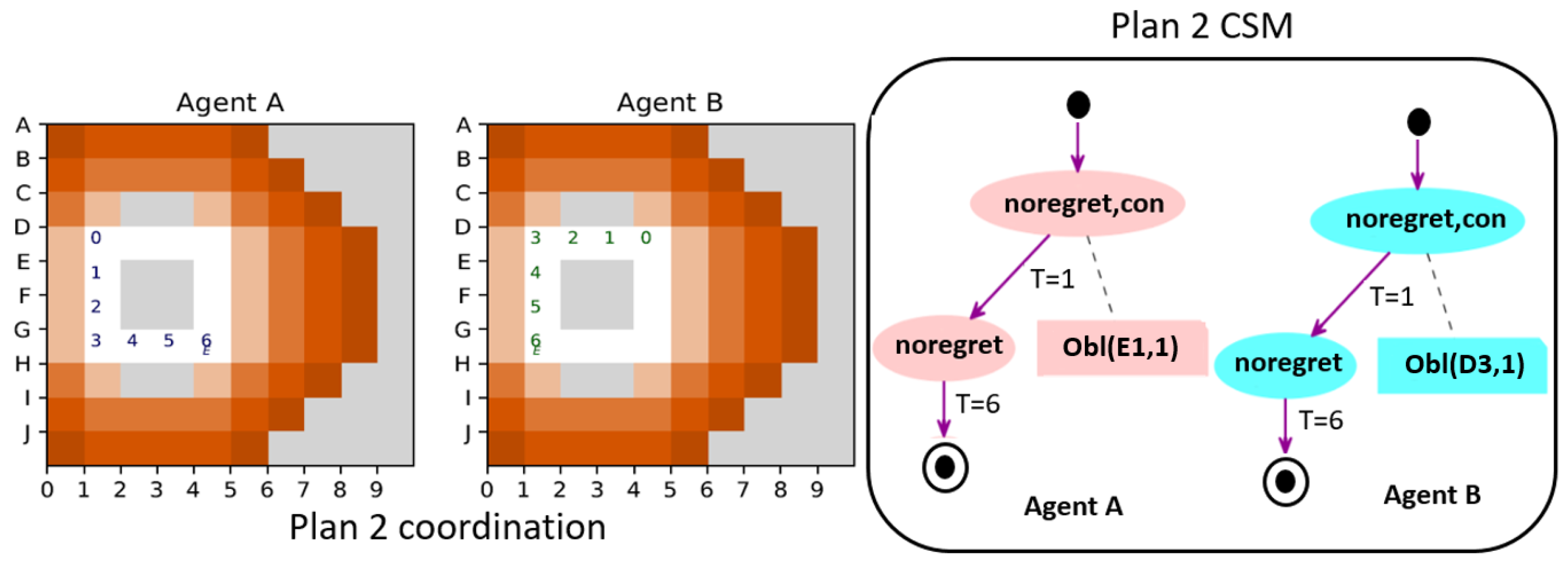
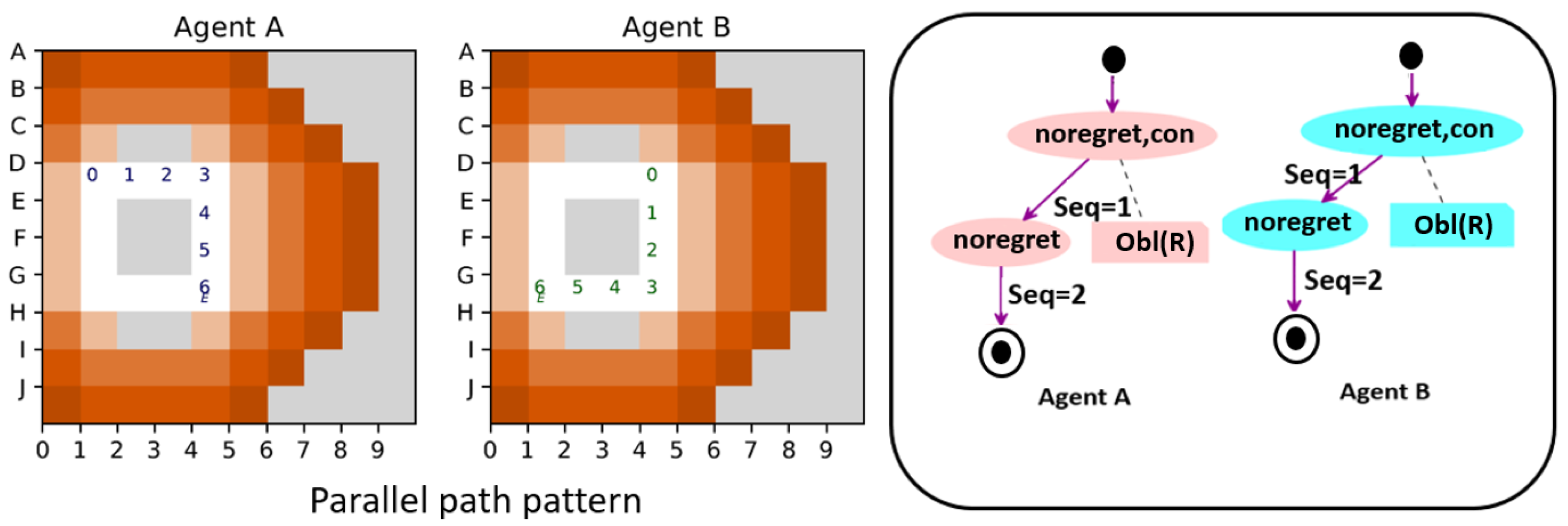
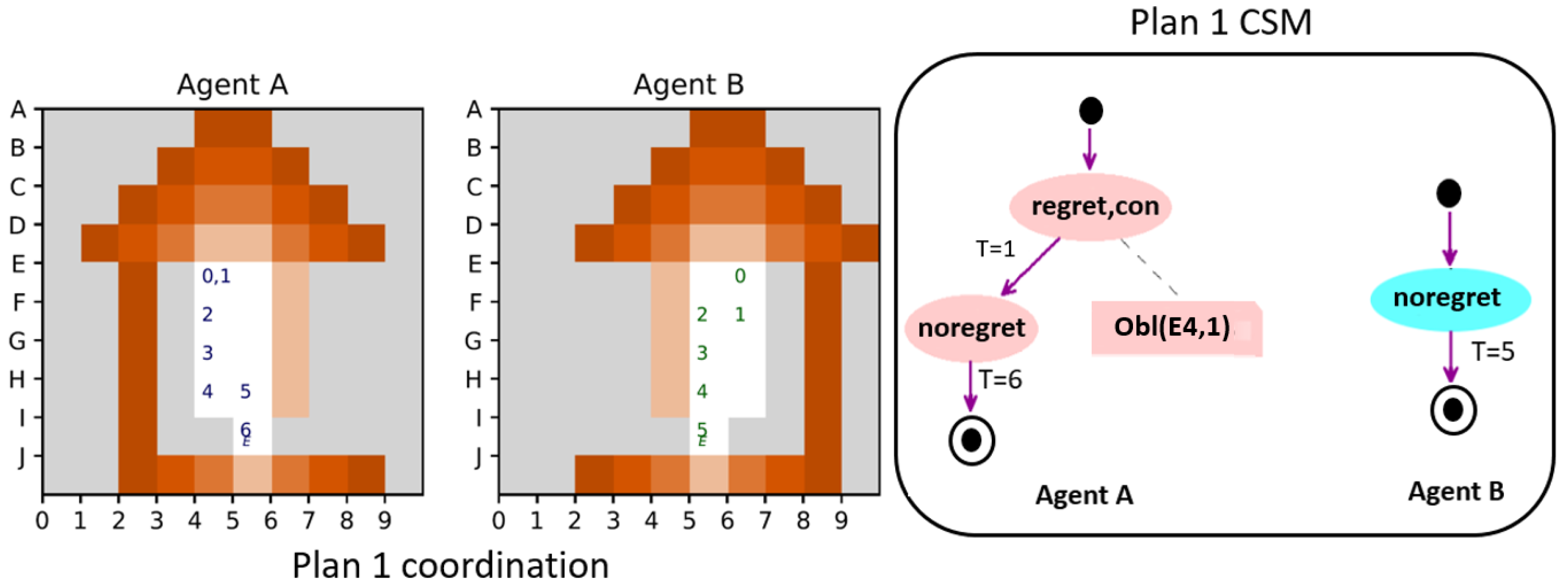
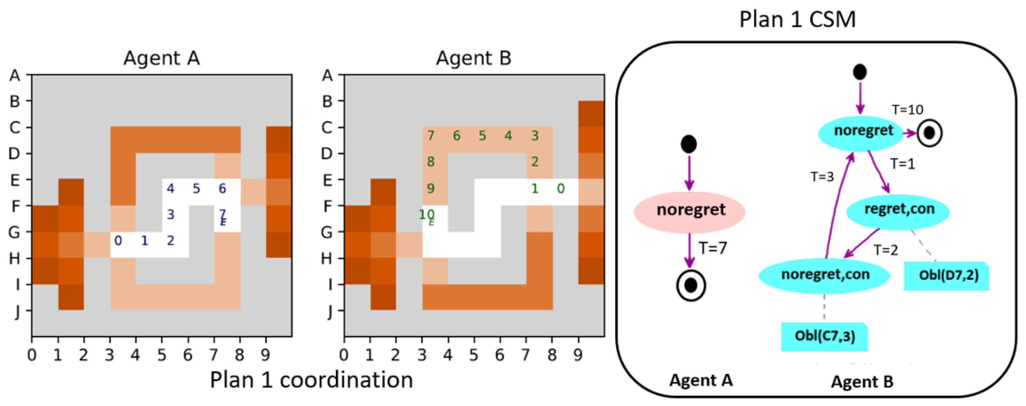
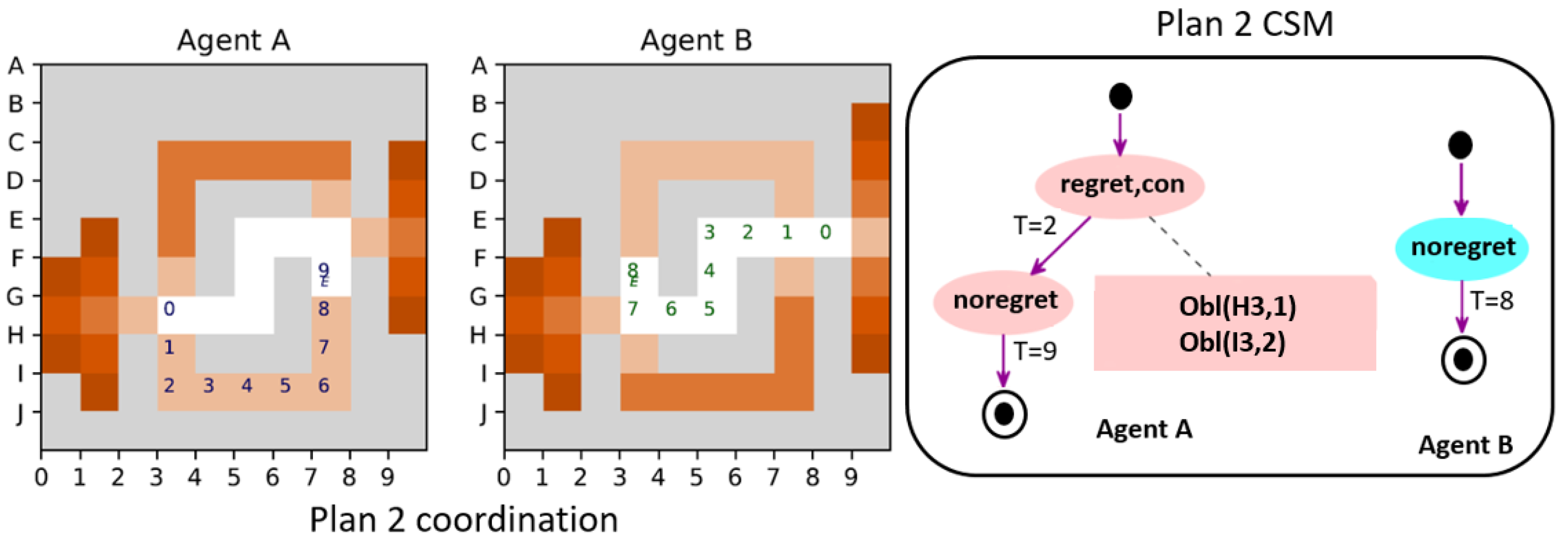
2.5. Coordination State Machines (CSMs)

A state machine encapsulates a system’s behaviour by delineating a finite set of states and defining transitions between them. These transitions are triggered by events, enabling a structured representation of sequential logic within a system. A candidate LCP selected by the norm entrepreneur agent is abstracted into a state machine model (we refer to this as a coordination state machine), which can then be used across different matching scenarios. The coordination state machine contains a separate state machine for each agent.

The states in a coordination state machine encapsulate abstract movement options agents have at a given time. There are two dimensions of these options and their cross product results in three states (as one combination is not possible). These options are abstracted, i.e., when an agent moves from one state to another the state machine does not specify exactly where it is going. Instead, the CSM specifies constraints on the agent’s location at specific time points. These constraints induce the same behaviour as the LCP under the assumption that the agent will always make an optimal choice from the allowed options.

The two dimensions of these movement options are as follows:

1.

Whether or not they must incur regret when they move, compared to the optimal action from the current location;

2.

Whether their movements are constrained or unconstrained.

The two state machines in a coordination state machine have the following components:

• A set of states: (“noregret ”, “noregret,con”, “regret,con”)

  ⁻

  noregret: when an agent is in this state, it is free to choose an optimal path, i.e., it does not need to incur regret;

  ⁻

  noregret,con”: When an agent is in this state, it does not need to incur regret. However, the coordination requires the agent to constrain its movements;

  ⁻

  “regret,con”: When an agent is in this state, the coordination requires the agent to incur regret by choosing a suboptimal action. The agent’s movement choices are also constrained.

• Movement constraints are associated with the states “noregret,con” and “regret,con”. These states are associated with sets of obligation and/or prohibition constraints. The syntax for these two types of constraints are shown in

  Table 1. The constraints in coordination state machines.

  Notation	Description	Example
  $Proh(\mathbf{R},\mathbf{T})$	“Proh” denotes that agents are prohibited from occupying specified locations for a given time interval; R is a range of cells with format $[C_1:C_n]$. Singleton cell ranges may be written as a single cell identifier, e.g., A1; T is a set of timesteps with format $[T_1:T_n]$. Singleton time intervals may be written as a single timepoint, e.g., T1.	$Proh\left(\right[D4:G4],[1:4\left]\right)$
  $Obl(\mathbf{R},\mathbf{T})$	“Obl” denotes that agents are obliged to move only within a range of cells for a given time interval; R is a range of cells with format $[C_1:C_n]$. Singleton cell ranges may be written as a single cell identifier, e.g., A1; T is a set of timesteps with format $[T_1:T_n]$. Singleton time intervals may be written as a single timepoint, e.g., T1.	$Obl\left(\right[A5:C6],[6:9\left]\right)$

  ;
• Transitions are identified by the timesteps: $1,2,\dots ,n$.

We assume that self-transitions to the same state are allowed for any time point not shown on an outgoing transition and omit these from our state machine diagrams. Although, the cross product of two independent dimensions would result in four states, only three states exists in the CSM’s state machines. There is no separate “regret” state because a regret state implies that the optional move is not allowed; so there must be a constraint on movement at that state, which is the state “regret,con”. The constraint may just prohibit the optimal moves, but it could specify a specific required suboptimal move to be taken. Algorithm 1 defines the process to construct a coordination state machine from an LCP, given the two agents’ value matrices, the set of possible actions, and each agent’s sequence of movements in the LCP (its “LCP path”).

Algorithm 1 Function to construct a coordination state machine.

1: Input: Value matrices: $V_A$ and $V_B$, a list of actions A and LCP paths: $lc{p}_A$ and $lc{p}_B$

2:

3: function ConstructCSM($V_A,V_B,A,lc{p}_A,lc{p}_B$)

4:      movement_map_A←ComputeMoveOptions$(V_A,A,lc{p}_A)$  ▹ Compute move options for agent A

5:      movement_map_B←ComputeMoveOptions$(V_B,A,lc{p}_B)$   ▹ Compute move options for agent B

6:      sm_A←ConstructSM(movement_map_A)  ▹ Construct an SM for agent A

7:      sm_B←ConstructSM(movement_map_B)   ▹ Construct an SM for agent B

8:      $\mathrm{csm}\leftarrow$(sm_A,sm_B)

9:      return csm

10:

11: function ComputeMoveOptions($V,A,\mathrm{lcp}$)

12:      movement_map$\leftarrow \mathrm{empty}\mathrm{dictionary}$

13:      for each cell C in lcp do

14:        $\mathrm{options}\leftarrow \underset{a\in \mathrm{A}}{argmax}\left\{V\left(\mathrm{move}(a,C)\right)\right\}$  ▹ Find optimal moves from C

15:        $\mathrm{choice}\leftarrow$ the next cell in lcp after C, or None if C is the last cell

16:        movement_map[C]$\leftarrow (\mathrm{options},\mathrm{choice})$

17:      return movement_map

18:

19: function ConstructSM(movement_map)

20:      sm←InitializeStateMachine$\left(‘\mathrm{noregret}’,‘\mathrm{regret},\mathrm{con}’,‘\mathrm{noregret},\mathrm{con}’,‘\mathrm{end}’\right)$  ▹ Create a state machine

21:      path_states$\leftarrow \left[\right]$

22:      for tstep, (_, desc) in enumerate(movement_map.items()) do

23:          $\mathrm{options}\leftarrow \mathrm{desc}\left[0\right]$

24:          $\mathrm{choice}\leftarrow \mathrm{desc}\left[1\right]$

25:          if $\mathrm{choice}\mathrm{is}\mathrm{None}$ then    ▹ Compute state for each move

26:              $\mathrm{state}\leftarrow ‘\mathrm{end}’$

27:          else if $\mathrm{choice}\mathrm{in}\mathrm{options}\mathrm{and}\mathrm{len}\left(\mathrm{options}\right)>1$ then

28:              $\mathrm{state}\leftarrow ‘\mathrm{noregret},\mathrm{con}’$

29:          else if $\mathrm{choice}\mathrm{in}\mathrm{options}$ then

30:              $\mathrm{state}\leftarrow ‘\mathrm{noregret}’$

31:          else

32:              $\mathrm{state}\leftarrow ‘\mathrm{regret},\mathrm{con}’$

33:        Add(state, path_states)

34:        $\mathrm{constraints}\leftarrow \mathrm{empty}\mathrm{dictionary}$

35:        if length(options) >1 then    ▹ Compute constraints

36:            constraint ← (“obl”,desc[1],tstep + 1)

37:            if state ∈ keys(constraints) then

38:                constraints[state].add(constraint)

39:            else

40:                $\mathrm{constraints}\left[\mathrm{state}\right]\leftarrow \left\{\mathrm{constraint}\right\}$

41:      SetInitialState(sm, path_states[0])   ▹ Set the SM’s initial state

42:      $\mathrm{transitions}\leftarrow \left[\right]$

43:      for i←0 to len(path_states) −1 do      ▹ Compute transitions

44:         current←path_states[i]

45:         next_state←current_states[i+1]

46:         if current≠next_state then

47:            $\mathrm{event}\leftarrow \mathrm{i}+1$   ▹ This represents a step of the LCP

48:            transitions.append({‘source’:current,‘target’:next_state,‘events’:[event]})

49:      SetTransitions($\mathrm{sm},\mathrm{transitions}$)

50:      return sm

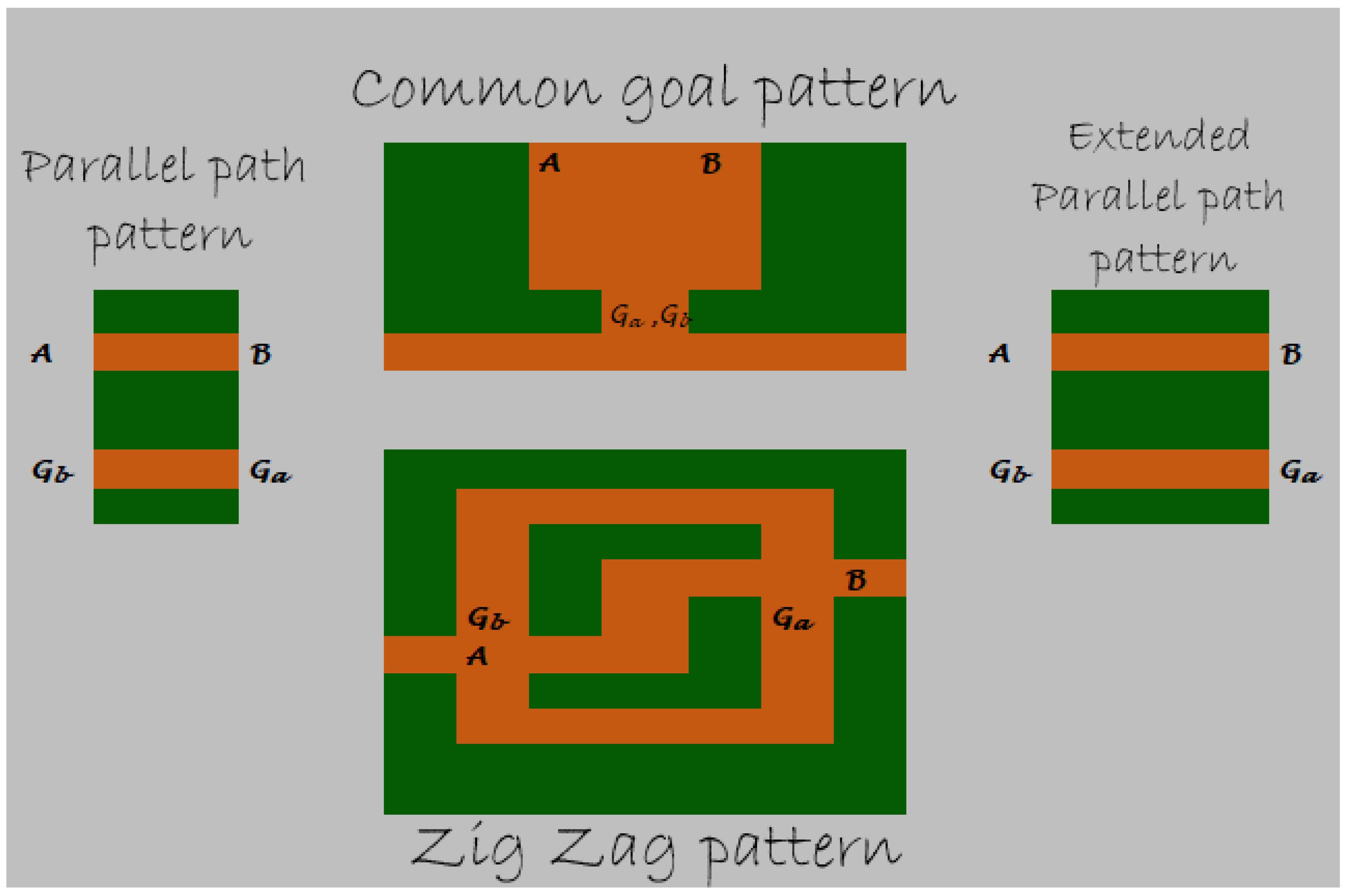
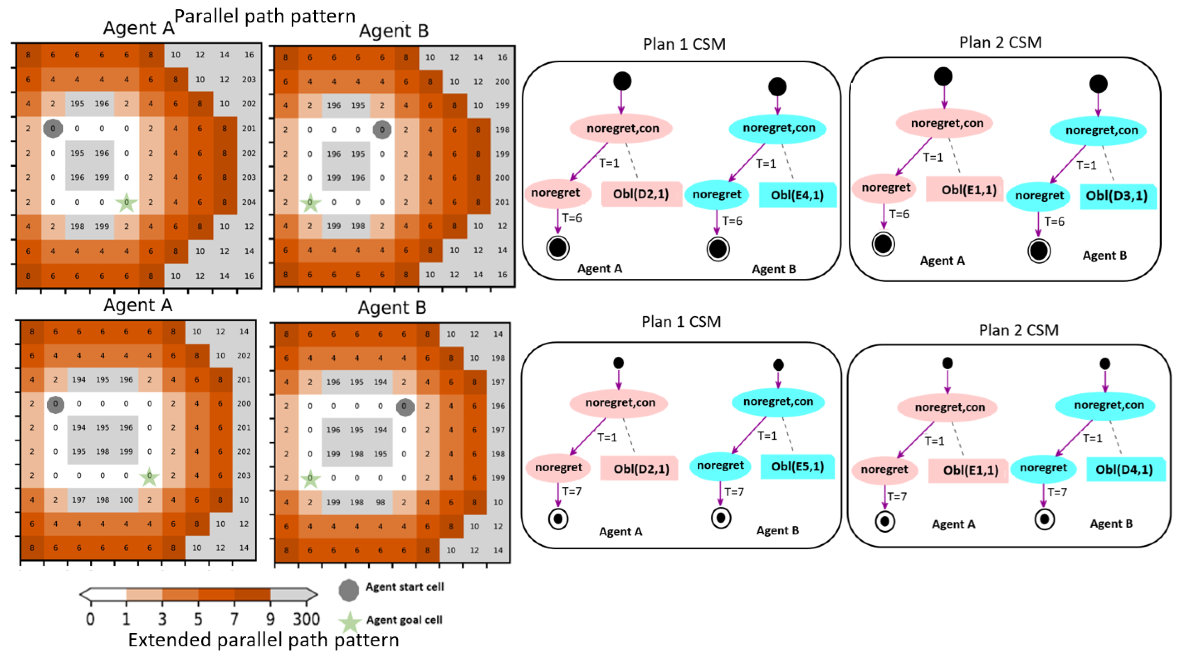
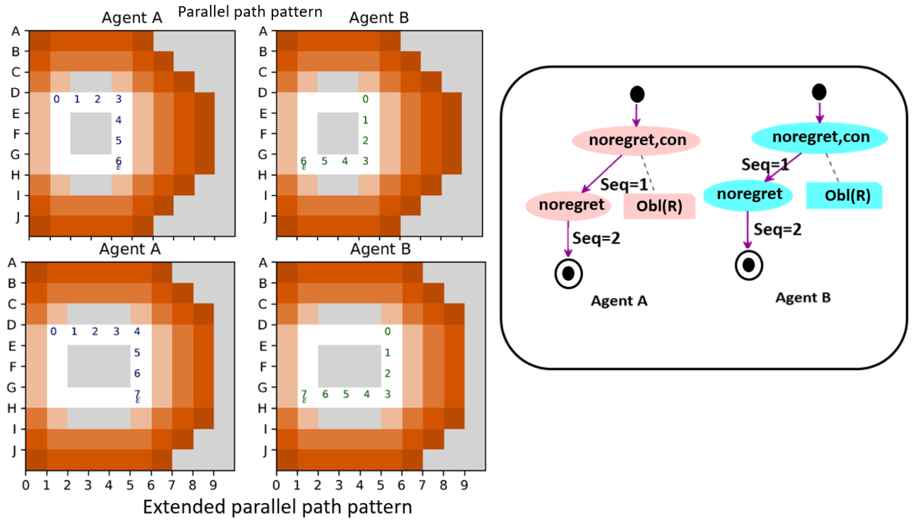
2.5.1. Parallel Path Pattern Plan

From the regret landscapes in Figure 6, we can infer that agents A and B each have two optimal paths to reach their respective goals. However, if both the agents decide to take the same route, i.e., if agent A moves to cell D2 and agent B moves to cell D3, their choices would result in a collision. Hence, the possible coordination plans require agents to choose non-overlapping optimal paths. Even though agents do not incur extra regret while choosing either of the optimal paths, they are constrained from entering one at a particular time. Figure 7 and Figure 8 illustrate the two local coordination plans and their abstraction as a CSM.

In Figure 7, both agents A and B start in the noregret,con state where they remain for one timestep and the agents are free to move optimally thereafter. At timestep 1, agent A is obliged to move to D2 and agent B is obliged to move to E4. After timestep 1, agents’ movements are not constrained as we assume that agents will move optimally thereafter.

2.5.2. Cross-Scenario CSMs

Until now, we have looked at abstracting a local coordination plan that agents agree upon while encountering a potential interference. However, these abstractions incorporate timesteps, which are specific to each pattern. We intend to further extend these abstractions away from specific timesteps. By doing so, the abstract notations could be reused across different matching patterns.

Figure 9 presents phase 2 of abstraction—the cross-scenario CSM for the parallel path pattern. The set of transitions Seq = 1, Seq = 2, …, Seq = n represents the state change sequence. A state change sequence encapsulates the timestep transitions. The “R” represents a region on which the constraints are applicable. The examples shown contain variables for the contents of the constraints, and these will be computed when matching a previously used CSM (in this abstracted form) to a new interference situation. This matching process will be the focus of the next stage of our research.

2.6. Examples

Let us now consider the remaining patterns from Figure 2. Figure 10, Figure 11 and Figure 12 show the regret of agents A and B for the extended parallel path pattern, common goal pattern, and zigzag pattern. The higher the saturation of a colour in the regret landscapes, the higher the regret. In Figure 10, there are two optimal paths around a more costly central region. In Figure 11, both agents have two optimal paths of which one path is the same for both. In Figure 12, both agents have a common optimal path and suboptimal paths that go around a costly central region.

Figure 13, Figure 14, Figure 15, Figure 16, Figure 17 and Figure 18 show a state machine model for each pattern from Figure 2. The left-hand side of these figures shows the coordination plans that the norm entrepreneur agent computed to resolve the potential interference. These plans are superimposed on their respective regret landscapes. For brevity, for patterns that have more than two coordination plans, we illustrated only two of them. Despite the norm entrepreneur presenting one plan from the set of Pareto-optimal plans it generates, we present two to illustrate how abstraction can exhibit similarity across various plans and patterns. The right-hand side of Figure 7, Figure 8 and Figure 13, Figure 14, Figure 15, Figure 16, Figure 17 and Figure 18 shows the abstraction using the coordination state machine. The figures show two different state machines, which correspond to agent A and B, respectively, for the same coordination plan.

2.6.1. Extended Parallel Path Pattern

The extended parallel path pattern is an elongated version of the parallel path pattern (discussed in Section 4). These two patterns are almost identical, with the difference being their duration and the constraints imposed.

Figure 13 and Figure 14 can be interpreted in the same manner as discussed in Section 2.5.1. We can observe that the two coordination patterns lead to a coordination state machine with the same structure.

Figure 19 illustrates the cross-scenario CSM for the extended parallel path pattern. It is evident that when we abstract from specific timesteps, the cross-scenario CSM for both the parallel path pattern and the extended parallel path pattern share identical cross-scenario CSMs. See Figure 9.

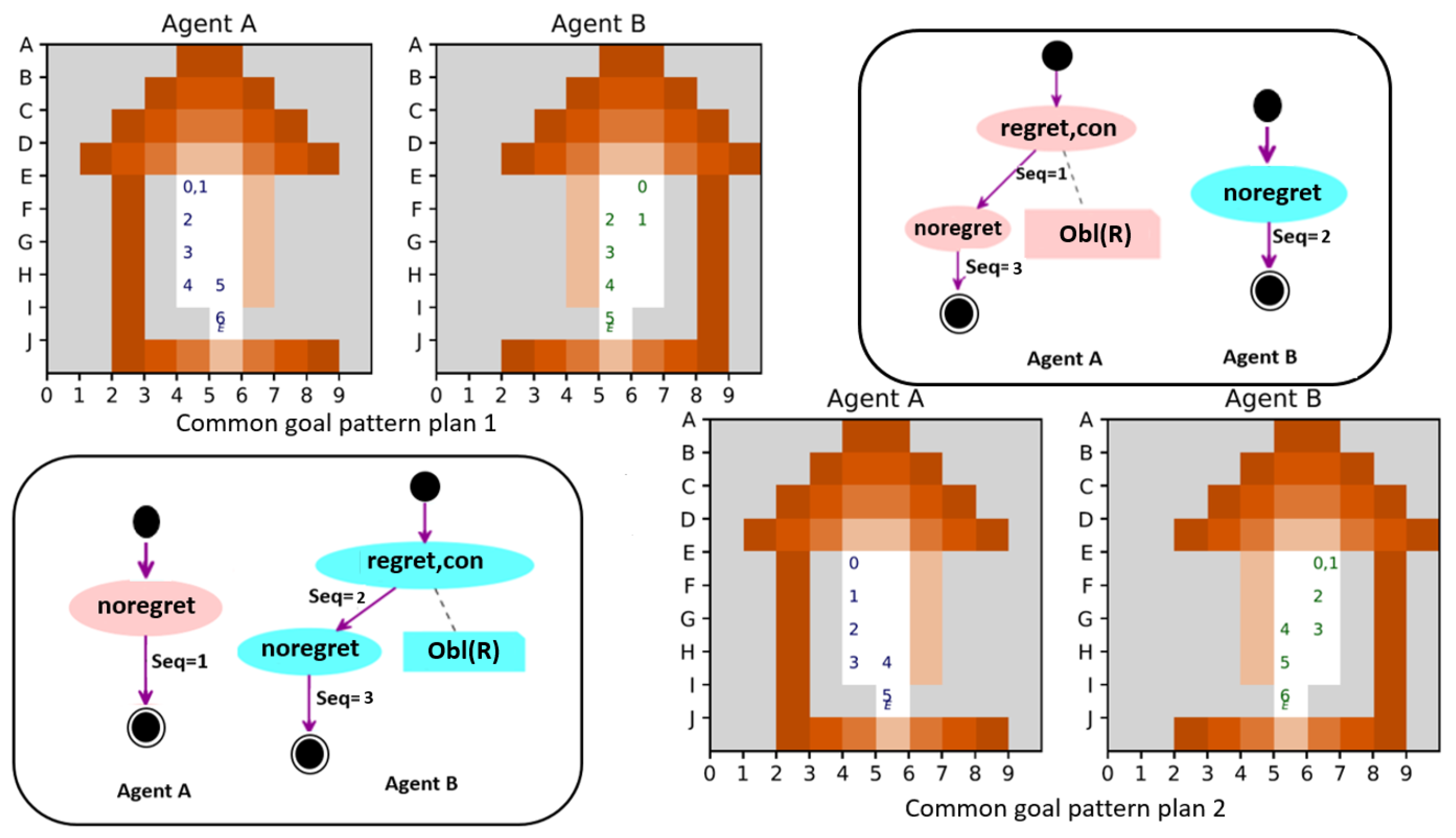
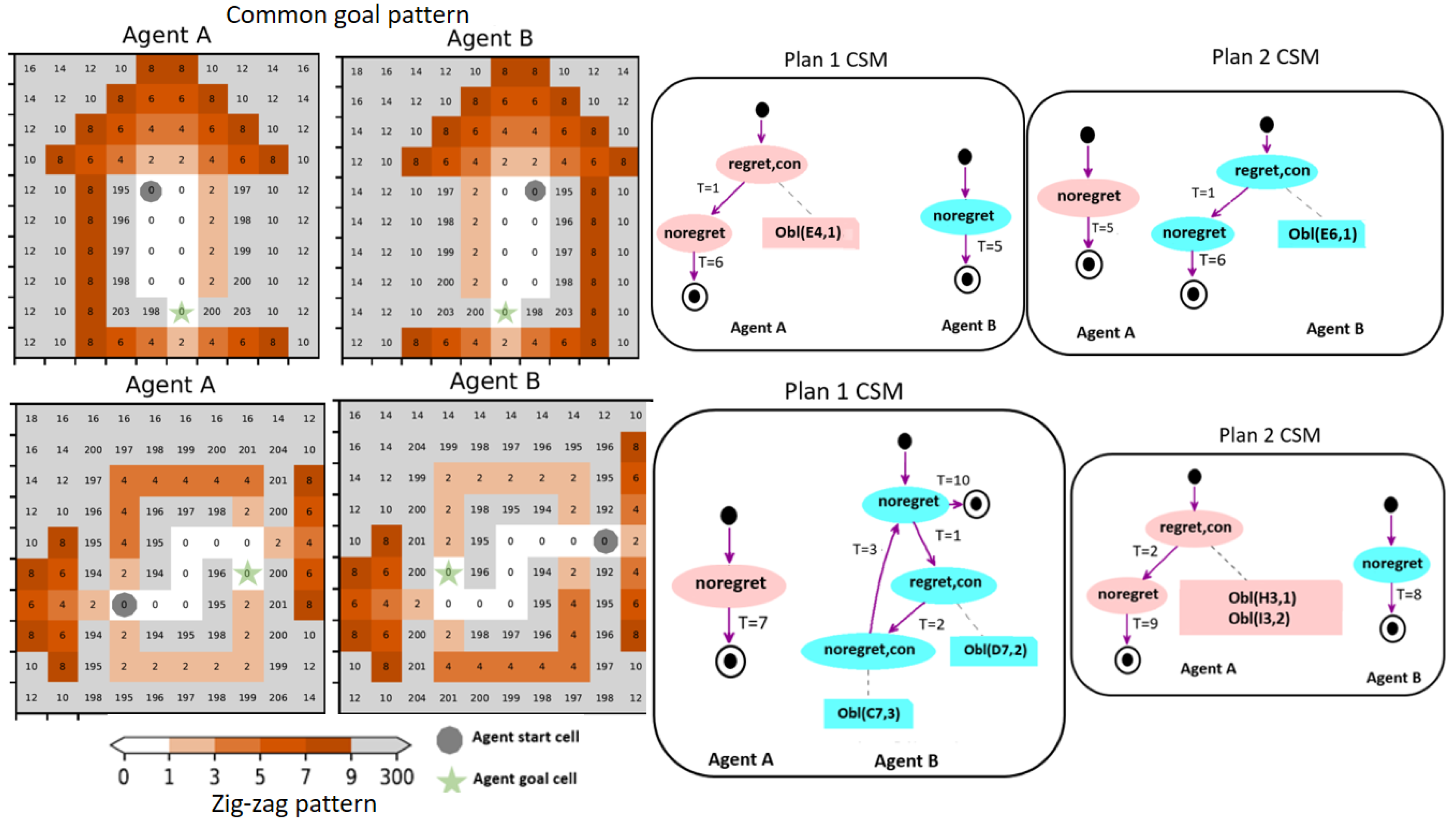
2.6.2. Common Goal Pattern

Unlike the coordination plans discussed in Figure 7, Figure 8, Figure 13 and Figure 14 where both agents initially have constrained movements, the coordination plans in Figure 15 and Figure 16 have one agent moving optimally and unconstrained while the other moves optimally but constrained.

In Figure 15, agent B is free to move optimally and unconstrained. For example, agent B could either move to E5 or F6 at timestep 1, while movement for agent A is restricted. Agent A is obliged to stay at E4 at timestep 1. This allows agent B to manoeuvre freely. Conversely, in Figure 16, restricting agent B to a region at timestep 1 allows agent A to move freely towards its goal.

Figure 20 depicts the cross-scenario CSM for these plans for the common goal pattern. It is noticeable that the agents experiencing regret in both plans share the same CSM, while those following the optimal path exhibit similar CSMs.

2.6.3. Zigzag Pattern

Unlike the patterns discussed so far where the agents have more than one optimal path to reach their goal, the zigzag pattern plans in Figure 17 and Figure 18 have agents with only one shared optimal path. As a consequence, when one agent moves optimally, the other is obliged to incur regret and follow a suboptimal path to reach its goal. For example in Figure 17, while agent A moves optimally without any constraints, agent B is obliged to move only in region D7 to C7 during the timesteps 2 and 3 (hence, the states “regret” and “noregret,con”). Even though agent B is obliged to incur regret at timestep 2, by timestep 4, it moves back to a “noregret” state. This is because, an agent incurring regret would incur the regret in the first few timesteps after it deviates from an optimal path to its suboptimal path. Once it incurs all the regret, thereafter it can move optimally. Hence, the transition $regret,con\stackrel{\mathrm{t}=4}{\to }noregret.$

Figure 21 illustrates the cross-scenario CSM for the zigzag pattern. To demonstrate the versatility of cross-scenario CSMs across different patterns, we focus on displaying the cross-scenario CSM of plan 2, as it mirrors the CSM of the common goal pattern. It is evident that the cross-scenario CSM for plan 2 resembles the cross-scenario CSM of plan 1 and plan 2 for the common goal patterns in Figure 20.

2.7. Executing a CSM

Once an agent receives a CSM, it retrieves the constraints of its current state from the CSM. The agent then calculates its possible optimal moves based on its current location and chooses a move from that, adhering to the constraints retrieved. Once the move is chosen, the agent then dispatches an event, signalling to the state machine that a particular event has occurred. The state machine then evaluates the transitions associated with that event. If the move is valid, the state machine transitions to the new state. If the move violates the constraints, an error will be raised, indicating that the agent’s movement violated the constraints, terminating cooperative execution of the CSM. Otherwise, the agent proceeds with the transition to the next state in the CSM and repeats the dispatch process until the ’end’ state is reached.

We confirmed that Algorithm 1 generates the CSM for the parallel path pattern plan 2 shown in Figure 8. Figure 22 shows the execution of this CSM by agent A. The figure uses a 0-based two-dimensional coordinate system instead of cell labels such as A0 (which maps to $(0,0)$). The agent begins by retrieving the constraints from the CSM for its initial movement and decides to move to position (4, 1), adhering to the constraints of that state. Subsequently, it continues without encountering any further constraints and successfully reaches the goal location (6, 4), as shown below.

The agent’s initial position is (3, 1).

• Timestep 1: The agent is in the state ’noregret,con’ at position (3, 1). A constraint is present requiring the agent to reach position (4, 1). The agent chooses to move to position (4, 1);
• Timestep 2: The agent is now in the state ’noregret’ at position (4, 1). No constraints are present. The agent is free to move optimally and chooses to move to position (5, 1);
• Timestep 3: The agent is still in the state ’noregret’ at position (5, 1). No constraints are present. The agent is free to move optimally and chooses to move to position (6, 1);
• Timestep 4: The agent is still in the state ’noregret’ at position (6, 1). No constraints are present. The agent is free to move optimally and chooses to move to position (6, 2);
• Timestep 5: The agent is still in the state ’noregret’ at position (6, 2). No constraints are present. The agent is free to move optimally and chooses to move to position (6, 3);
• Timestep 6: The agent is still in the state ’noregret’ at position (6, 3). No constraints are present. The agent chooses to move to position (6, 4), successfully reaching its goal.

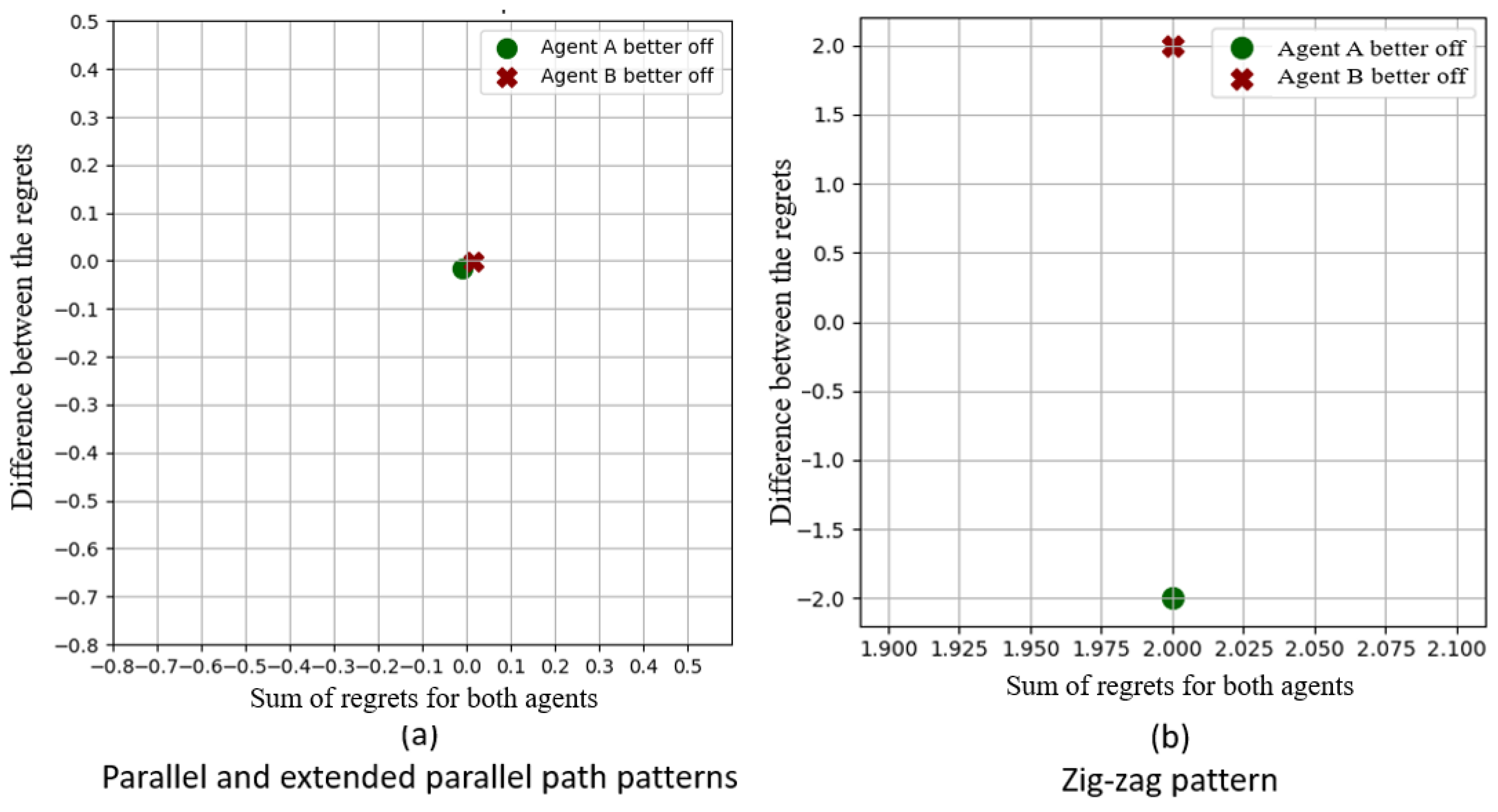
3. Results

We considered four scenarios (Figure 2) within an environment where agents encounter potential interferences. Local coordination planning was then utilised to generate Pareto-optimal plans to resolve these interferences. Subsequently, the Pareto frontier solutions for the selected scenarios were plotted as points on a 2D coordinate system, as depicted in Figure 23 and Figure 24.

In Figure 23 and Figure 24, the sum of regrets for both agents and the difference between their regrets is plotted. Regret here refers to the difference between the cost of an agent’s part of a local coordination plan and that of its optimal plans. The figures’ colour schemes use green to denote situations where agent A (the entrepreneur agent) experiences the least regret and red where the opposite is true. These figures illustrate the nature of the Pareto frontier of LCPs as a trade-off between social welfare (where a smaller sum of regrets is preferred) and fairness (where a smaller difference between the agents’ regrets is preferred).

The example coordination scenarios fall into two categories based on the solutions from the local coordination planning.

Category 1 depicted in Figure 23 illustrates scenarios where there are only two solutions available. Figure 23a depicts cases where both agents incur no regret. For example, in the parallel path pattern and the extended parallel path pattern in Figure 2, both the agents incur no regret following either of the plans. This happens when agents have more than one optimal plan and they have to refrain from crossing paths. Figure 23b pertains to scenarios where two solutions exist: one where agent A benefits more and another where agent B does. The points are jittered to illustrate two distinct plans.

Category 2 includes scenarios with multiple solutions for the potential interference. Figure 24 illustrates the common goal pattern scenario. This addresses scenarios with a large number of Pareto frontier solutions, which can be divided into two categories: green denotes 50 plans where agent A benefits more, while red represents the remaining 50 plans where agent B fares better. Interestingly, these 100 solutions can be abstracted to two distinct groups, which allow the norm entrepreneur agent to propose just two solutions, consolidating the possibilities in each group. In scenarios where multiple plans exist, each agent can opt for the most favourable plan from their respective set of options. Once both agents have made their selections, a distributed coin toss can then be utilised to determine the final choice among them.

Abstracting solutions with a CSM yielded reusable state machines applicable to various matching patterns. The abstraction depicted in Figure 25 reveals that both the parallel path pattern and the extended parallel path pattern share a coordination state machine, differing only in time intervals. The extended parallel path pattern essentially extends the parallel path pattern. Interestingly, the plan 2 CSM in the zigzag pattern and the common goal pattern depicted in Figure 26 also demonstrate a similar abstraction.

Figure 27 presents the cross-scenario CSMs for the parallel path pattern and the extended parallel path pattern. We can see that the patterns have the same abstraction, allowing it to be reusable across patterns.

From Figure 28, we can observe that, unlike the parallel path and extended parallel path pattern, the common goal pattern and the zigzag pattern appear to be distinct and unrelated patterns. Despite this disparity, the the cross-scenario CSMs for these two patterns are identical from the agents’ perspective, except that the state machines for agents A and B are swapped.

4. Discussion

This paper presents a novel framework aimed at establishing norms to effectively manage interference among agents within decentralised environments. Our methodology differs significantly from the approaches previously utilised in this research domain. Rather than attempting to plan for every possible inter-agent interaction, which is often impractical, we advocate for a dynamic approach where agents address interference as it arises.

Firstly, by introducing norm entrepreneur agents, we provide a solution to the challenge of coordinating agents in a multi-agent system without relying on specially empowered entities. These norm entrepreneur agents dynamically identify local regions of coordination (ROCs) in which potential agent interferences may occur, and propose plans to prevent the interference.

Secondly, we address the question of representing agent coordination in a more generalisable manner. Through the generation of local coordination plans (LCPs) by norm entrepreneurs within ROCs, we move beyond the notion of coordination as a single joint action choice. These plans, abstracted and proposed to other agents, offer a flexible framework for resolving interference while accommodating the dynamic nature of decentralised environments.

We develop coordination state machines (CSM) to abstract local coordination plans to apply to a range of coordination problems. CSMs express constraints imposed on agents that have agreed to coordinate using that CSM and identify at which coordination steps the agents must incur regret compared to making individually optimal choices. We examine four distinct interference scenarios in the environment (Figure 2). The coordination state machines and the cross-scenario CSMs generated for these scenarios demonstrate that CSMs can be reused across different and unrelated patterns. Figure 9 and Figure 19 indicate that a single CSM can accommodate similar structured, elongated versions of a pattern. Figure 20 and Figure 21, although unrelated, share the same abstraction. Moreover, cross-scenario CSMs enable the abstraction of timesteps, consolidating various local coordination plans into one.

After the norm entrepreneur agent generates a set of Pareto-optimal LCPs and generalizes these into CSMs at subsequent stages, they proceed to the proposal and agreement phase. In situations where there is a single optimal CSM, with no agent incurring regret or where all regrets are equal and socially optimal, proposing this option is clearly advantageous. Otherwise, each agent has the liberty to choose the most favourable CSMs from their respective set of options. The agents then conduct a distributed coin toss to select one of these CSMs, allowing them to agree on outcomes without relying on a central authority. To ensure that the norm entrepreneur agent is not cherry picking the proposed CSMs, auditor agents can be introduced into the environment so agents can seek validation of a norm entrepreneur agent’s fairness. In environments where interference is frequent, agents will have an incentive to coordinate to avoid the costs of potentially repeated interference. Also, a reputation mechanism can be employed to inform agents whether they can trust that the other agent will likely conform to an agreed CSM. These mechanisms promote consensus building and cooperation among agents, fostering local coordination planning and making the NEMAS framework effective in addressing potential interferences in a distributed environment.

References

1. Sumner, W. Folkways: A Study of the Sociological Importance of Usages, Manners, Customs, Mores, and Morals; Good Press: Addison, TX, USA, 1906. [Google Scholar]
2. Kubler, D. On the Regulation of Social Norms. J. Law Econ. Organ. 2001, 17, 449–476. [Google Scholar] [CrossRef]
3. Sunstein, C.R. Social Norms and Social Roles. Columbia Law Rev. 1996, 96, 903–968. [Google Scholar] [CrossRef]
4. Finnemore, M.; Sikkink, K. International Norm Dynamics and Political Change. Int. Organ. 1998, 52, 887–917. [Google Scholar] [CrossRef]
5. Anavankot, A.M.; Cranefield, S.; Savarimuthu, B.T.R. Towards Norm Entrepreneurship in Agent Societies. In International Conference on Practical Applications of Agents and Multi-Agent Systems; Springer: Berlin/Heidelberg, Germany, 2023. [Google Scholar] [CrossRef]
6. Opp, K.D. When Do Norms Emerge by Human Design and When by the Unintended Consequences of Human Action?: The Example of the No-smoking Norm. Ration. Soc. 2002, 14, 131–158. [Google Scholar] [CrossRef]
7. Centola, D.; Baronchelli, A. The Spontaneous Emergence of Conventions: An Experimental Study of Cultural Evolution. Proc. Natl. Acad. Sci. USA 2015, 112, 1989–1994. [Google Scholar] [CrossRef] [PubMed]
8. Boella, G.; Torre, L.; Verhagen, H. Introduction to the Special Issue on Normative Multiagent Systems. Auton. Agents -Multi-Agent Syst. 2008, 17, 1–10. [Google Scholar] [CrossRef]
9. Shoham, Y.; Tennenholtz, M. On the Synthesis of Useful Social Laws for Artificial Agent Societies. In Proceedings of the Tenth National Conference on Artificial intelligence (AAAI’92), San Jose, CA, USA, 12–16 July 1992; pp. 276–281. [Google Scholar]
10. Morales, J.; López-Sánchez, M.; Rodríguez-Aguilar, J.; Wooldridge, M.; Vasconcelos, W. Automated Synthesis of Normative Systems. In Proceedings of the 12th International Conference on Autonomous Agents and Multiagent Systems, Saint Paul, MN, USA, 6–10 May 2013. [Google Scholar]
11. Morales, J.; López-Sánchez, M.; Rodríguez-Aguilar, J.; Wooldridge, M.; Vasconcelos, W. Minimality and simplicity in the on-line automated synthesis of normative systems. In Proceedings of the 13th International Conference on Autonomous Agents and Multiagent Systems, Paris, France, 5–9 May 2014; pp. 109–116. [Google Scholar]
12. Morales, J.; López-Sánchez, M.; Rodríguez-Aguilar, J.A.; Wooldridge, M.J.; Vasconcelos, W.W. Synthesising Liberal Normative Systems. In Proceedings of the Proceedings of the 2015 International Conference on Autonomous Agents and Multiagent Systems, Istanbul, Turkey, 4–8 May 2015; ACM: New York, NY, USA, 2015; pp. 433–441. [Google Scholar]
13. Morales, J.; Wooldridge, M.; Rodríguez-Aguilar, J.; López-Sánchez, M. Synthesising Evolutionarily Stable Normative Systems. Auton. Agents -Multi-Agent Syst. 2018, 32, 635–671. [Google Scholar] [CrossRef] [PubMed]
14. Alechina, N.; De Giacomo, G.; Logan, B.; Perelli, G. Automatic Synthesis of Dynamic Norms for Multi-Agent Systems. In Proceedings of the 19th International Conference on Principles of Knowledge Representation and Reasoning, Haifa, Israel, 31 July–5 August 2022; Volume 8, pp. 12–21. [Google Scholar] [CrossRef]
15. Riad, M.; Golpayegani, F. Run-Time Norms Synthesis in Multi-objective Multi-agent Systems. In Coordination, Organizations, Institutions, Norms, and Ethics for Governance of Multi-Agent Systems XIV; Theodorou, A., Nieves, J.C., Vos, M.D., Eds.; Springer: Berlin/Heidelberg, Germany, 2021; Volume 13239, Lecture Notes in Computer Science; pp. 78–93. [Google Scholar] [CrossRef]
16. Riad, M.; Golpayegani, F. A Normative Multi-objective Based Intersection Collision Avoidance System. In Smart Innovation, Systems and Technologies; Springer: Singapore, 2022; pp. 289–300. [Google Scholar] [CrossRef]
17. Riad, M.; Ghanadbashi, S.; Golpayegani, F. Run-Time Norms Synthesis in Dynamic Environments with Changing Objectives. In Proceedings of the Artificial Intelligence and Cognitive Science—30th Irish Conference, Munster, Ireland, 8–9 December 2022; Revised Selected Papers. Longo, L., O’Reilly, R., Eds.; Springer: Berlin/Heidelberg, Germany, 2022; Volume 1662, Communications in Computer and Information Science. pp. 462–474. [Google Scholar] [CrossRef]
18. Morris-Martin, A.; Vos, M.D.; Padget, J.A.; Ray, O. Agent-directed Runtime Norm Synthesis. In Proceedings of the Proceedings of the 2023 International Conference on Autonomous Agents and Multiagent Systems, London, UK, 29 May–2 June 2023. [Google Scholar] [CrossRef]
19. Morris-Martin, A.; De Vos, M.; Padget, J. A Norm Emergence Framework for Normative MAS–Position Paper. In Proceedings of the Coordination, Organizations, Institutions, Norms, and Ethics for Governance of Multi-Agent Systems XIII: International Workshops COIN 2017 and COINE 2020, Sao Paulo, Brazil, 8–9 May 2017; Virtual Event, 9 May 2020; Revised Selected Papers; Springer: Berlin/Heidelberg, Germany, 2021; pp. 156–174. [Google Scholar]
20. Morris-Martin, A.; Vos, M.D.; Padget, J.A. Norm Emergence in Multiagent Systems: A Viewpoint Paper. In Proceedings of the 19th International Conference on Autonomous Agents and Multiagent Systems, AAMAS’20, Auckland, New Zealand, 9–13 May 2020. [Google Scholar] [CrossRef]
21. Aldewereld, H.; Grossi, D.; Vázquez-Salceda, J.; Dignum, F. Designing Normative Behaviour Via Landmarks. In International Conference on Autonomous Agents and Multiagent Systems; Springer: Berlin/Heidelberg, Germany, 2005; number 3913 in Lecture Notes in Computer Science; pp. 157–169. [Google Scholar] [CrossRef]
22. Ben-Or, M.; Linial, N. Collective coin flipping, robust voting schemes and minima of Banzhaf values. In Proceedings of the 26th Annual Symposium on Foundations of Computer Science (sfcs 1985), Portland, OR, USA, 21–23 October 1985; pp. 408–416. [Google Scholar] [CrossRef]
23. Savarimuthu, B.T.R.; Cranefield, S. Norm creation, spreading and emergence: A survey of simulation models of norms in multi-agent systems. Multiagent Grid Syst. 2011, 7, 21–54. [Google Scholar] [CrossRef]
24. Balke, T.; Cranefield, S.; di Tosto, G.; Mahmoud, S.; Paolucci, M.; Savarimuthu, B.T.R.; Verhagen, H. Simulation and NorMAS. In Normative Multi-Agent Systems; Andrighetto, G., Governatori, G., Noriega, P., van der Torre, L.W.N., Eds.; Dagstuhl Follow-Ups, Schloss Dagstuhl—Leibniz-Zentrum für Informatik: Hatfield, UK, 2013; pp. 171–189. [Google Scholar] [CrossRef]
25. Kallenberg, L. Finite State and Action MDPS. In Handbook of Markov Decision Processes: Methods and Applications; Feinberg, E.A., Shwartz, A., Eds.; Springer: Berlin/Heidelberg, Germany, 2002; pp. 21–87. [Google Scholar] [CrossRef]
26. Mandow, L.; Pérez de la Cruz, J.L. Multiobjective A* Search with Consistent Heuristics. J. ACM 2010, 57, 1–25. [Google Scholar] [CrossRef]
Figure 1. A single-step coordination problem from Morales et al. [10].
Systems 12 00187 g001
Figure 2. The park layout (best viewed in colour). The figure illustrates the park layout, where green cells represent lawn areas, brown cells represent pathways, and grey cells represent open spaces. A and B indicate the current locations of the two agents, and G a and G b show their goal locations.
Systems 12 00187 g002
Figure 3. Overview of the norm entrepreneurship framework. The coloured arrows represent different local coordination plans.
Systems 12 00187 g003
Figure 4. The parallel path pattern. Green cells represent lawn areas, brown cells represent pathways, and grey cells represent open spaces. A and B indicate the current locations of the two agents, and G a and G b show their goal locations.
Systems 12 00187 g004
Figure 5. The Value matrix generated by the value iteration algorithm for Figure 4.
Systems 12 00187 g005
Figure 6. Regret landscapes for the parallel path pattern. The figure shows the regret landscapes of agents A and B for the parallel path pattern. The higher the saturation of a colour in the regret landscapes, the higher the regret.
Systems 12 00187 g006
Figure 7. Parallel path pattern plan 1. The figure shows the regret landscapes of agents A and B for the parallel path pattern. The higher the saturation of a colour in the regret landscapes, the higher the regret. The plans are superimposed on their respective regret landscapes. “0” refers to the starting point of the agent. The numbers 1 , 2 , 3 , refer to the steps the agent takes to reach its goal, and the numbers with a subscript “E” refer to the goal.
Systems 12 00187 g007
Figure 8. Parallel path pattern plan 2. This figure shows the regret landscapes of agents A and B for the parallel path pattern. The higher the saturation of a colour in the regret landscapes, the higher the regret. The plans are superimposed on their respective regret landscapes. “0” refers to the starting point of the agent. The numbers 1 , 2 , 3 , refer to the steps the agent takes to reach its goal, and the numbers with a subscript “E” refer to the goal.
Systems 12 00187 g008
Figure 9. Parallel path cross-scenario CSM. The figure shows the cross-scenario CSM of agents A and B for the parallel path pattern. The higher the saturation of a colour in the regret landscapes, the higher the regret. The plans are superimposed on their respective regret landscapes. “0” refers to the starting point of the agent. The numbers 1 , 2 , 3 , refer to the steps the agent takes to reach its goal, and the numbers with a subscript “E” refer to the goal. The set of transitions Seq = 1, Seq = 2, …, Seq = n represents the state change sequence.
Systems 12 00187 g009
Figure 10. Regret landscapes for the extended parallel path pattern. The figure shows the regret landscapes of agents A and B for the parallel path pattern. The higher the saturation of a colour in the regret landscapes, the higher the regret.
Systems 12 00187 g010
Figure 11. Regret landscapes for the common goal pattern. The figure shows the regret landscapes of agents A and B for the common goal pattern. The higher the saturation of a colour in the regret landscapes, the higher the regret.
Systems 12 00187 g011
Figure 12. Regret landscapes for the zig-zag pattern. The figure shows the regret landscapes of agents A and B for the zig-zag pattern. The higher the saturation of a colour in the regret landscapes, the higher the regret.
Systems 12 00187 g012
Figure 13. Extended parallel path pattern plan 1. The figure shows the regret landscapes of agents A and B for the extended parallel path pattern. The higher the saturation of a colour in the regret landscapes, the higher the regret. The plans are superimposed on their respective regret landscapes. “0” refers to the starting point of the agent. The numbers 1 , 2 , 3 , refer to the steps the agent takes to reach its goal, and the numbers with a subscript “E” refer to the goal.
Systems 12 00187 g013
Figure 14. Extended parallel path pattern plan 2. The figure shows the regret landscapes of agents A and B for the extended parallel path pattern. The higher the saturation of a colour in the regret landscapes, the higher the regret. The plans are superimposed on their respective regret landscapes. “0” refers to the starting point of the agent. The numbers 1 , 2 , 3 , refer to the steps the agent takes to reach its goal, and the numbers with a subscript “E” refer to the goal.
Systems 12 00187 g014
Figure 15. Common goal pattern plan 1. The figure shows the regret landscapes of agents A and B for the common goal pattern. The higher the saturation of a colour in the regret landscapes, the higher the regret. The plans are superimposed on their respective regret landscapes. “0” refers to the starting point of the agent. The numbers 1 , 2 , 3 , refer to the steps the agent takes to reach its goal, and the numbers with a subscript “E” refer to the goal.
Systems 12 00187 g015
Figure 16. Common goal pattern plan 2. The figure shows the regret landscapes of agents A and B for the common goal pattern. The higher the saturation of a colour in the regret landscapes, the higher the regret. The plans are superimposed on their respective regret landscapes. “0” refers to the starting point of the agent. The numbers 1 , 2 , 3 , refer to the steps the agent takes to reach its goal, and the numbers with a subscript “E” refer to the goal.
Systems 12 00187 g016
Figure 17. Zigzag pattern plan 1 The figure shows the regret landscapes of agents A and B for the zig-zag pattern. The higher the saturation of a colour in the regret landscapes, the higher the regret. The plans are superimposed on their respective regret landscapes. “0” refers to the starting point of the agent. The numbers 1 , 2 , 3 , refer to the steps the agent takes to reach its goal, and the numbers with a subscript “E” refer to the goal.
Systems 12 00187 g017
Figure 18. Zigzag pattern plan 2. The figure shows the regret landscapes of agents A and B for the zig-zag pattern. The higher the saturation of a colour in the regret landscapes, the higher the regret. The plans are superimposed on their respective regret landscapes. “0” refers to the starting point of the agent. The numbers 1 , 2 , 3 , refer to the steps the agent takes to reach its goal, and the numbers with a subscript “E” refer to the goal.
Systems 12 00187 g018
Figure 19. Extended parallel path cross-scenario CSM. The figure shows the cross-scenario CSM of agents A and B for the extended parallel path pattern. The higher the saturation of a colour in the regret landscapes, the higher the regret. The plans are superimposed on their respective regret landscapes. “0” refers to the starting point of the agent. The numbers 1 , 2 , 3 , refer to the steps the agent takes to reach its goal, and the numbers with a subscript “E” refer to the goal. The set of transitions Seq = 1, Seq = 2, …, Seq = n represents the state change sequence.
Systems 12 00187 g019
Figure 20. Common goal pattern cross-scenario CSM. The figure shows the cross-scenario CSM of agents A and B for the common goal pattern. The higher the saturation of a colour in the regret landscapes, the higher the regret. The plans are superimposed on their respective regret landscapes. “0” refers to the starting point of the agent. The numbers 1 , 2 , 3 , refer to the steps the agent takes to reach its goal, and the numbers with a subscript “E” refer to the goal. The set of transitions Seq = 1, Seq = 2, …, Seq = n represents the state change sequence.
Systems 12 00187 g020
Figure 21. Zigzag pattern cross-scenario CSM. The figure shows the cross-scenario CSM of agents A and B for the zig-zag pattern. The higher the saturation of a colour in the regret landscapes, the higher the regret. The plans are superimposed on their respective regret landscapes. “0” refers to the starting point of the agent. The numbers 1 , 2 , 3 , refer to the steps the agent takes to reach its goal, and the numbers with a subscript “E” refer to the goal. The set of transitions Seq = 1, Seq = 2, …, Seq = n represents the state change sequence.
Systems 12 00187 g021
Figure 22. Trace of an agent executing a CSM.
Systems 12 00187 g022
Figure 23. Regret for agents A and B across LCPs—two solution category (the points are jittered to allow them all to be seen). We use green to denote situations where agent A experiences the least regret and red where agent B experiences the least regret.
Systems 12 00187 g023
Figure 24. Regret for agents A and B across LCPs—multiple solution category (the points are jittered to allow them all to be seen). We use green to denote situations where agent A experiences the least regret and red where agent B experiences the least regret.
Systems 12 00187 g024
Figure 25. Coordination state machines for the parallel path pattern and extended parallel path pattern. The figure shows the cross-scenario CSM of agents A and B. The higher the saturation of a colour in the regret landscapes, the higher the regret. The plans are superimposed on their respective regret landscapes. “0” refers to the starting point of the agent. The numbers 1 , 2 , 3 , refer to the steps the agent takes to reach its goal, and the numbers with a subscript “E” refer to the goal. The circle represents the agent’s start cell and the star represents the agent’s goal cell.
Systems 12 00187 g025
Figure 26. Coordination state machines for the common goal and zigzag pattern. The figure shows the cross-scenario CSM of agents A and B. The higher the saturation of a colour in the regret landscapes, the higher the regret. The plans are superimposed on their respective regret landscapes. “0” refers to the starting point of the agent. The numbers 1 , 2 , 3 , refer to the steps the agent takes to reach its goal, and the numbers with a subscript “E” refer to the goal. The circle represents the agent’s start cell and the star represents the agent’s goal cell.
Systems 12 00187 g026
Figure 27. Parallel path and extended parallel path pattern cross-scenario CSM. The higher the saturation of a colour in the regret landscapes, the higher the regret. The plans are superimposed on their respective regret landscapes. “0” refers to the starting point of the agent. The numbers 1 , 2 , 3 , refer to the steps the agent takes to reach its goal, and the numbers with a subscript “E” refer to the goal. The set of transitions Seq = 1, Seq = 2, …, Seq = n represents the state change sequence.
Systems 12 00187 g027
Figure 28. Common goal and zigzag pattern cross-scenario CSM. The higher the saturation of a colour in the regret landscapes, the higher the regret. The plans are superimposed on their respective regret landscapes. “0” refers to the starting point of the agent. The numbers 1 , 2 , 3 , refer to the steps the agent takes to reach its goal, and the numbers with a subscript “E” refer to the goal. The set of transitions Seq = 1, Seq = 2, …, Seq = n represents the state change sequence.
Systems 12 00187 g028