Quantifying the Complexity of Nodes in Higher-Order Networks Using the Infomap Algorithm

Abstract

Accurately quantifying the complexity of nodes in a network is crucial for revealing their roles and network complexity, as well as predicting network emergent phenomena. In this paper, we propose three novel complexity metrics for nodes to reflect the extent to which they participate in organized, structured interactions in higher-order networks. Our higher-order network is built using the BuildHON+ model, where communities are detected using the Infomap algorithm. Since a physical node may contain one or more higher-order nodes in higher-order networks, it may simultaneously exist in one or more communities. The complexity of a physical node is defined by the number and size of the communities to which it belongs, as well as the number of higher-order nodes it contains within the same community. Empirical flow datasets are used to evaluate the effectiveness of the proposed metrics, and the results demonstrate their efficacy in characterizing node complexity in higher-order networks.

1. Introduction

The complexity of a network reflects the extent to which its nodes participate in organized, structured interactions [1]. Highly complex networks achieve a balance between order and disorder, exhibiting both regularity and randomness, and have a high likelihood of emergent phenomena [2]. Accurately quantifying network complexity is critical for revealing network characteristics and predicting network emergent phenomena [3]. Common network complexity metrics based on topology [4,5] attempt to calculate the number of nodes or interactions in a network, highlighting the significance of node complexity as a key component of network complexity. Therefore, accurate quantification of node complexity can reveal the role of nodes within a network well and help to predict network emergent phenomena [6]. In addition, the complexity of a node can be defined as the extent to which it participates in organized, structured interactions [7].

Recently, many higher-order network models [8,9,10,11] have been proposed as more accurate representations of underlying data, focusing on features that first-order network models fail to capture. By incorporating higher-order attributes during the network-construction process, higher-order networks can describe complex interactions among multiple nodes that go beyond pairwise connections, thereby enhancing the effectiveness of network-analysis methods [12,13]. This improvement arises because previous studies, when constructing networks from sequential data, typically overlooked relationships beyond pairwise node connections, implicitly assuming a first-order Markov process. This assumption led to the omission of significant higher-order information present in the original data [14]. To address this issue, Rosvall et al. [15] developed a second-order Markov network model to capture dynamic behaviors, which not only revealed actual travel patterns in air traffic but also uncovered propagation patterns within citation networks. Subsequently, Xu et al. [16] proposed the BuildHON algorithm, which extracts patterns or rules with frequencies high enough to be considered significant and constructs higher-order networks through two steps: rule extraction and network rewiring. Building on this, Saebi et al. [17] introduced the BuildHON+ algorithm, which controls the growth of higher-order rules through dynamic thresholds, thus reducing the time and space complexity compared to the BuildHON algorithm. Additionally, some studies have proposed preliminary quantitative descriptions of node complexity in higher-order networks. For example, Rosvall et al. [15] used the Infomap algorithm within second-order Markov networks to identify hub cities in air traffic and to uncover multidisciplinary journals in scientific communication. Xu et al. [16] applied the Infomap algorithm in higher-order networks to effectively locate the Freeport of Malta—one of Europe’s busiest ports. Fu et al. [18] utilized the PageRank algorithm within the multi-scale higher-order dependency networks to identify key nodes within the global liner shipping network, revealing the dual circular economy models in the relevant countries.

Motivated by these works, we propose three quantitative complexity metrics for nodes in higher-order networks [17] using the Infomap algorithm [19,20]. First, we build a higher-order network from flow data and detect communities using the Infomap algorithm. Next, we define three complexity metrics for nodes based on the number and size of the communities to which they belong, as well as the number of higher-order nodes contained within the same community. Finally, we demonstrate the effectiveness of our proposed complexity metrics using empirical flow datasets.

2. Node Complexity Metrics Definition

2.1. Node Complexity Metrics Definition in First-Order Networks

First-order network (FON) is defined as a graph $G=(V,E)$, where $V=\{a,b,c,\dots \}$ denotes the physical node set, and E represents the physical edge set. Community in a first-order network is defined as a node set $O_i,i=1,2,3,\dots ,n$, then $V=O_1\cup O_2\cup O_3\cup \cdots \cup O_n$. When $i\ne j$, we have $O_i\cap O_j=⌀$.

Based on community detection in first-order network, three node complexity metrics are defined below. Firstly, let ${\delta }_i\left(x\right)$ be defined as:

$${\delta }_i\left(x\right)=\left\{\begin{array}{ccc}\hfill 1,& \hfill \hfill & \hfill x\in O_i\\ \hfill 0,& \hfill \hfill & \hfill x\notin O_i\end{array}\right..$$

(1)

Then, the node complexity metrics in first-order networks are defined as follows:

$$C_1\left(x\right)=\sum _{i=1}^n{\delta }_i\left(x\right),$$

(2)

$$C_2\left(x\right)=\sum _{i=1}^n{\delta }_i\left(x\right)·lg\left|O_i\right|,$$

(3)

$$C_3\left(x\right)=\sum _{i=1}^n{\delta }_i\left(x\right)·lg{\displaystyle \frac{|O_i|}{|x\cap O_i|}},$$

(4)

where $x\in V$, and $|O_i|$ denotes the size of the community $O_i$.

2.2. Rationality Analysis of Node Complexity Metrics in FON

• The more communities a node belongs to, the higher its complexity. $C_1\left(x\right)$ represents the number of communities to which node x belongs. In FON, since $i\ne j$ implies $O_i\cap O_j=⌀$, $C_1\left(x\right)=1$ is constant when using the Infomap algorithm.
• The larger the size of the communities to which a node belongs, the higher its complexity. Based on $C_1\left(x\right)$, $C_2\left(x\right)$ is positively correlated with the size of the communities to which node x belongs. To make the data distribution more uniform and reduce the impact of outliers, we introduce the logarithmic function $lg(·)$ to measure node complexity. Specifically, when $\left|O_i\right|=1$, meaning the community contains only one node, $C_2\left(x\right)=0$. When $|O_i|=1$, then $C_2\left(x\right)=0$.
• The greater the proportion of a node within its community, the lower its complexity. Building on $C_1\left(x\right)$ and $C_2\left(x\right)$, $C_3\left(x\right)$ also considers the proportion of node x within its community, which is negatively correlated with complexity. When $x\cap O_i\ne ⌀$, meaning $\left|x\cap O_i\right|=1$, then $C_3\left(x\right)=C_2\left(x\right)$. When $x\cap O_i=⌀$, meaning $x\notin O_i$, then $\left|x\cap O_i\right|=0$. When $\left|x\cap O_i\right|=0$, set the denominator to 1. This ensures that Equation (4) remains valid without affecting the experimental results.

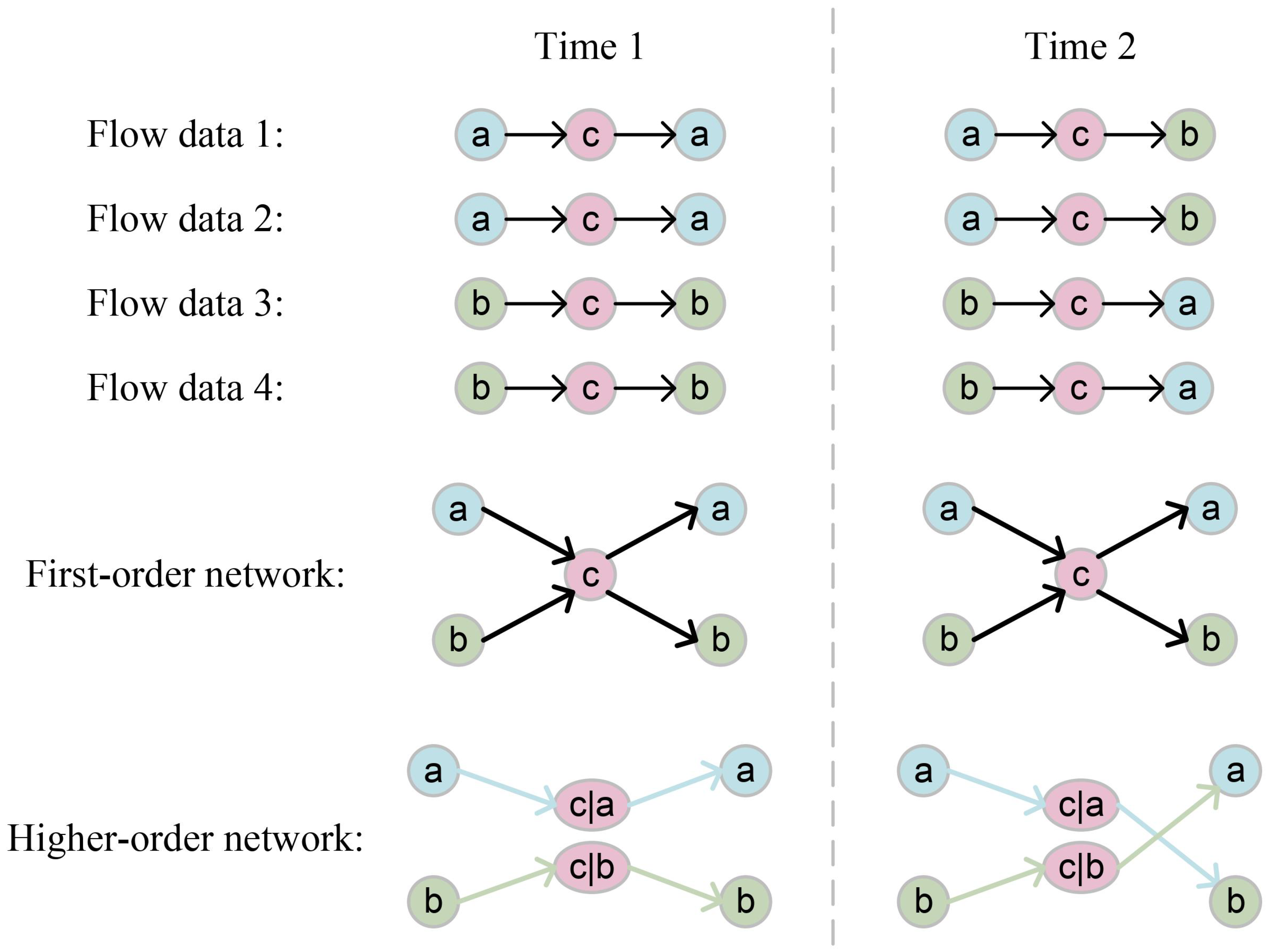
2.3. Higher-Order Network Model

To represent flow data accurately, the BuildHON+ model [17] could convert multivariate sequential interactions among multiple nodes into higher-order nodes and their edges. The model consists of two steps: higher-order node construction and edge rewire.

The construction of higher-order nodes depends on the frequency and transition probability distribution entropy of multivariate sequences. Firstly, we introduce the relevant concepts [16,18]: the order of a network is equal to the order of the highest-order node in the network, the order of a node corresponds to the length of its associated multivariate sequence, and the count of a node indicates the number of occurrences of its corresponding multivariate sequence. For example, the multivariate sequence $b\to c$ appears 4 times in the network, and its corresponding higher-order node is $s=c|b$. The order of node s is 2, and its count is 4. Secondly, only when the multivariate sequence count exceeds a certain threshold, is it considered to exist. For example, if the multivariate sequence count is $n_{c\to b\to a}=4$ and the threshold is $n_0=2$, then the multivariate sequence $c\to b\to a$ is considered to exist. Thirdly, the Kullback–Leibler divergence $D_{KL}$ is introduced as a measure of information gain:

$$D_{KL}(Q\parallel P)=\sum _{i=1}^n{q}_i\times {log}_2{\displaystyle \frac{q_i}{p_i}},$$

(5)

where $P=\left[p_1,p_2,\cdots ,p_n\right]$ represents the transition probability distribution for the current higher-order node $s_1=a|b.c.\cdots .x$, and $Q=\left[q_1,q_2,\cdots ,q_n\right]$ for the higher-order subsequence $s_2=a|b.c.\cdots .x.\cdots .y$. $o\left(s_1\right)$ and $o\left(s_2\right)$ denotes the orders of the higher-order node $s_1$ and the higher-order subsequence $s_2$, respectively, with $o\left(s_1\right)<o\left(s_2\right)$.

Meanwhile, the dynamic threshold is denoted as

$$\delta ={\displaystyle \frac{o\left(s_2\right)}{{log}_2(1+n\left(s_2\right))}},$$

(6)

where $o\left(s_2\right)$ denotes the order of subsequence $s_2$, and $n\left(s_2\right)$ is the count of subsequence $s_2$. When $D_{KL}(Q\parallel P)>\delta$, subsequence $s_2$ becomes a new candidate higher-order node and replaces the old candidate higher-order node $s_1$. Otherwise, subsequence $s_1$ remains the candidate higher-order node.

The rewire of edges aims to establish the connection between higher-order nodes. First, construct a first-order network based on all first-order nodes and their edges. Second, for each higher-order node, construct a path from the corresponding first-order node to it. For example, for higher-order node $a|b.c$, a path $c\to b|c\to a|b.c$ will be constructed. Third, construct the edges between different paths. For example, for path $c\to b|c\to a|b.c$, there is $a|b.c\to b$. There must exist a higher-order node $\tilde{x}$, which satisfies $\tilde{x}=max\left\{b\right|a.b,b|a,b\}$, then $a|b.c\to \tilde{x}$.

In order to visualize a higher-order network model, Figure 1 shows the comparison of first- and higher-order network models. Based on flow data in time 1, node a passes through node c and goes back to node a, as does node b. Based on flow data in time 2, node a passes through node c and goes back to node b; meanwhile, node b passes through node c and goes back to node a. A higher-order network model clearly reflects the above information, but a first-order network model does not, which demonstrates the accuracy of higher-order network models.

2.4. Node Complexity Metrics Definition in Higher-Order Networks

A higher-order network (HON) can be defined as a graph $\tilde{G}=(\tilde{V},\tilde{E})$, where $\tilde{V}=\{a,b,c,\dots \}$ denotes the higher-order node set; for any $\tilde{x}\in \tilde{V}$, there must exist $x\in V$, such that $\tilde{x}\in x=$$\left\{x\right|,x|a,x|b,\dots \}$, and $\tilde{E}$ represents the higher-order edge set. Community in a higher-order network is defined as a node set ${\tilde{O}}_i,i=1,2,3,\dots ,n$, then $\tilde{V}={\tilde{O}}_1\cup {\tilde{O}}_2\cup {\tilde{O}}_3\cup \cdots \cup {\tilde{O}}_n$. When $i\ne j$, we have ${\tilde{O}}_i\cap {\tilde{O}}_j=⌀$.

Based on community detection in higher-order networks, three higher-order node complexity metrics are defined below. Firstly, let ${\tilde{\delta }}_i\left(\tilde{x}\right)$ be defined as:

$${\tilde{\delta }}_i\left(\tilde{x}\right)=\left\{\begin{array}{ccc}\hfill 1,& \hfill \hfill & \hfill \tilde{x}\in {\tilde{O}}_i\\ \hfill 0,& \hfill \hfill & \hfill \tilde{x}\notin {\tilde{O}}_i\end{array}\right..$$

(7)

Then, the node complexity metrics in higher-order networks are defined as follows:

$${\tilde{C}}_1\left(x\right)=\sum _{\tilde{x}\in x}\sum _{i=1}^n{\tilde{\delta }}_i\left(\tilde{x}\right),$$

(8)

$${\tilde{C}}_2\left(x\right)=\sum _{\tilde{x}\in x}\sum _{i=1}^n{\tilde{\delta }}_i\left(\tilde{x}\right)·lg\left|{\tilde{O}}_i\right|,$$

(9)

$${\tilde{C}}_3\left(x\right)=\sum _{x\in \tilde{x}}\sum _{i=1}^n{\tilde{\delta }}_i\left(\tilde{x}\right)·lg{\displaystyle \frac{|{\tilde{O}}_i|}{|x\cap {\tilde{O}}_i|}}.$$

(10)

For first-order networks, $\tilde{x}=x$ and ${\tilde{O}}_i=O_i$, so that

$${\tilde{\delta }}_i\left(\tilde{x}\right)=\left\{\begin{array}{c}1,\tilde{x}\in {\tilde{O}}_i\\ 0,\tilde{x}\notin {\tilde{O}}_i\end{array}\right.=\left\{\begin{array}{c}1,x\in O_i\\ 0,x\notin O_i\end{array}.\right.$$

(11)

Combined with Equation (1), it is easy to find that ${\tilde{\delta }}_i\left(\tilde{x}\right)={\delta }_i\left(x\right)$. Therefore, the three higher-order node complexity metrics are suitable for first-order networks as well.

2.5. Rationality Analysis of Node Complexity Metrics in HON

Similar to the analysis of node complexity metrics in FON, since a physical node in HON may correspond to multiple higher-order nodes, it can therefore appear in multiple communities. Based on this, we conducted the following analysis:

• The more communities a physical node belongs to, the higher its complexity.
• The larger the communities a physical node belongs to, the higher its complexity. ${\tilde{C}}_2\left(x\right)$ is positively correlated with both the number and size of the communities to which node x belongs.
• The greater the proportion of a physical node within a community, the lower its complexity. ${\tilde{C}}_3\left(x\right)$ also considers positive correlations with the number and size of the communities to which node x belongs, as well as a negative correlation with the proportion of node x within its communities.

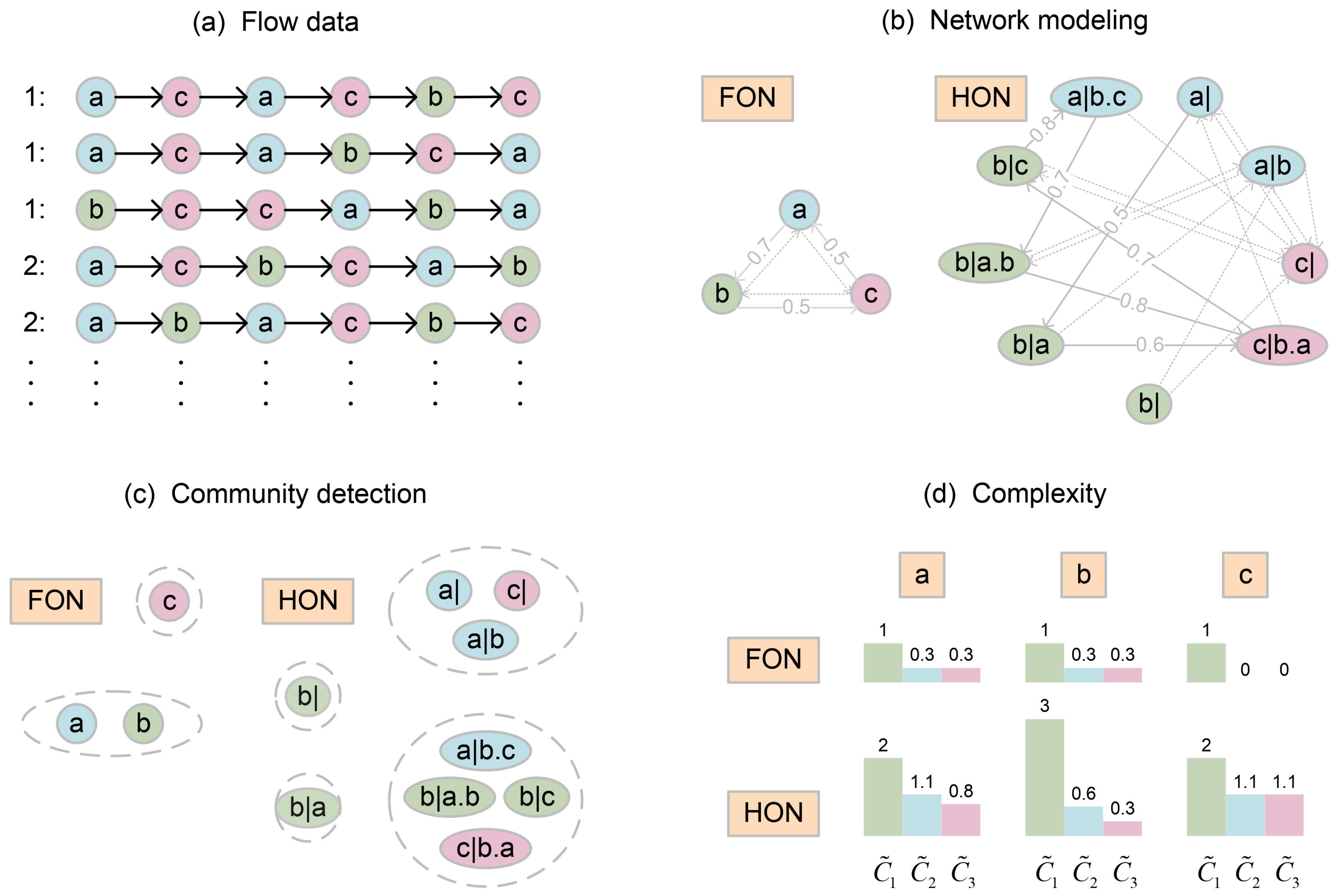
2.6. A Sample of Node Complexity Quantification Process

To introduce the quantification process of node complexity, we present a sample in Figure 2. Using the BuildHON+ model, we first build both a first- and higher-order network based on flow data. We then detect communities using the Infomap algorithm in networks. Finally, we calculate node complexity using the above three node complexity metrics, which reveals node characteristics better in a higher-order network than in a first-order network. For example, node b has the most higher-order interactions based on the number of communities it belongs to, so its complexity ${\tilde{C}}_1\left(b\right)$ should be the highest. That is true in higher-order networks, but not in first-order networks.

3. Results and Analysis

3.1. Data Descriptions

To verify the effectiveness of above three complexity metrics, we introduce three empirical flow datasets, Enron, railway and citation, as the experimental datasets. The detailed descriptions of these flow datasets are as follows:

• Enron [15,21]: This flow dataset refers to 116,525 emails between 146 users in Enron Corporation. It was originally made public and posted to the web by the Federal Energy Regulatory Commission during its investigation.
• Railway: This flow dataset covers 4458 high-speed train numbers going through 672 stations of 34 provinces in China in 2016, collected from http://www.12306.cn/ (accessed on 20 January 2024).
• Citation [22]: This flow dataset contains 8,850,334 citations in 668,383 papers in 19 journals of the American Physical Society (APS) by the end of 2020. Among them, the maximum length of the citation flow does not exceed 2.

3.2. Results in Enron Flow Dataset

Firstly, we divide Enron Corporation staff in the Enron flow dataset into three categories: ordinary employees, middle-level managers and senior leaders. The middle-level managers include the managers and directors who are in the middle leadership; meanwhile the senior leaders are the top leaders of the corporation, such as the CEO, presidents, vice presidents, managing directors, and chief operating officers.

Based on the Enron flow dataset, first- and higher-order Enron networks are built by the BuildHON+ model, where top 50 staff in complexity are picked up. Because the senior leaders participate in the most communities, they have the highest complexity. In contrast, the ordinary employees have the lowest complexity. In a word, the more senior leaders and middle-level managers in the top 50, the better the complexity metric. Figure 3 shows the number of ordinary employees, middle-level managers, and senior leaders occupied in the top 50 nodes ranked by three complexity metrics in Enron networks. The red area denotes the number of senior leaders, and the green area repersents the number of middle-level managers. The sum of above two areas ranked by ${\tilde{C}}_1,{\tilde{C}}_2,{\tilde{C}}_3$ in higher-order networks is far greater than that in first-order networks. That is to say, the above three complexity metrics perform better in higher-order networks than in first-order networks.

The top 20 staff with high complexity of ${\tilde{C}}_1,{\tilde{C}}_2,{\tilde{C}}_3$ in Enron networks are shown in

Table 1. The top 20 staff with high complexity of ${\tilde{C}}_1$ in Enron networks.

Enron—FON				Enron—HON
ID	Name	Position	${\tilde{\mathit{C}}}_{\mathbf{1}}$	ID	Name	Position	${\tilde{\mathit{C}}}_{\mathbf{1}}$
1	kuykendall-t	Trader	1	47	lavorato-j	CEO	9
2	kitchen-l	President	1	2	kitchen-l	President	6
3	geaccone-t	-	1	82	grigsby-m	Manager	6
4	cash-m	-	1	21	sager-e	-	5
5	merriss-s	-	1	33	shively-h	Vice President	5
6	linder-e	-	1	48	perlingiere-d	-	5
7	griffith-j	-	1	96	kaminski-v	Manager	5
8	mccarty-d	Vice President	1	136	neal-s	Vice President	5
9	rapp-b	-	1	4	cash-m	-	4
10	lay-k	CEO	1	13	mann-k	-	4
11	keavey-p	-	1	14	tycholiz-b	Vice President	4
12	love-p	-	1	19	scott-s	-	4
13	mann-k	-	1	28	buy-r	Manager	4
14	tycholiz-b	Vice President	1	58	kuykendall-t	-	4
15	pereira-s	-	1	65	haedicke-m	Managing Director	4
16	meyers-a	-	1	67	kean-s	Vice President	4
17	hendrickson-s	-	1	86	hyvl-d	-	4
18	solberg-g	-	1	128	keiser-k	-	4
19	scott-s	-	1	23	hodge-j	Managing Director	3
20	schoolcraft-d	-	1	41	martin-t	Vice President	3

,

Table 2. The top 20 staff with high complexity of ${\tilde{C}}_2$ in Enron networks.

Enron—FON				Enron—HON
ID	Name	Position	${\tilde{C}}_2$	ID	Name	Position	${\tilde{C}}_2$
3	geaccone-t	-	1.204	47	lavorato-j	CEO	11.222
8	mccarty-d	Vice President	1.204	82	grigsby-m	Manager	7.824
9	rapp-b	-	1.204	2	kitchen-l	President	7.665
20	schoolcraft-d	-	1.204	21	sager-e	-	6.474
42	corman-s	Vice President	1.204	33	shively-h	Vice President	6.410
53	blair-l	-	1.204	96	kaminski-v	Manager	6.402
72	watson-k	-	1.204	136	neal-s	Vice President	6.061
77	harris-s	-	1.204	14	tycholiz-b	Vice President	5.678
83	mcconnell-m	-	1.204	13	mann-k	-	5.474
90	lokay-m	Administrative Asisstant	1.204	58	taylor-m	-	5.432
95	donoho-l	-	1.204	67	kean-s	Vice President	5.424
111	hyatt-k	Director	1.204	48	perlingiere-d	-	5.403
119	horton-s	President	1.204	4	cash-m	-	5.131
120	lokey-t	Manager	1.204	128	keiser-k	-	5.073
124	ybarbo-p	-	1.204	65	haedicke-m	Managing Director	5.044
134	hayslett-r	Vice President	1.204	86	hyvl-d	-	4.900
5	merriss-s	-	1.079	28	buy-r	Manager	4.868
6	linder-e	-	1.079	41	martin-t	Vice President	4.591
16	meyers-a	-	1.079	117	mclaughlin-e	-	4.591
18	solberg-g	-	1.079	129	steffes-j	Vice President	4.470

and

Table 3. The top 20 staff with high complexity of ${\tilde{C}}_3$ in Enron networks.

Enron—FON				Enron—HON
ID	Name	Position	${\tilde{C}}_3$	ID	Name	Position	${\tilde{C}}_3$
3	geaccone-t	-	1.204	47	lavorato-j	CEO	27.073
8	mccarty-d	Vice President	1.204	2	kitchen-l	President	23.218
9	rapp-b	-	1.204	82	grigsby-m	Manager	18.596
20	schoolcraft-d	-	1.204	58	taylor-m	-	16.654
42	corman-s	Vice President	1.204	72	watson-k	-	15.950
53	blair-l	-	1.204	46	dasovich-j	Executive	15.608
72	watson-k	-	1.204	77	harris-s	-	15.163
77	harris-s	-	1.204	14	tycholiz-b	Vice President	14.205
83	mcconnell-m	-	1.204	86	hyvl-d	-	14.113
90	lokay-m	Administrative Asisstant	1.204	67	kean-s	Vice President	14.080
95	donoho-l	-	1.204	43	nemec-g	-	13.825
111	hyatt-k	Director	1.204	21	sager-e	-	13.812
119	horton-s	President	1.204	35	jones-t	-	13.679
120	lokey-t	Manager	1.204	129	steffes-j	Vice President	13.523
124	ybarbo-p	-	1.204	39	fossum-d	Vice President	13.269
134	hayslett-r	Vice President	1.204	128	keiser-k	-	12.567
5	merriss-s	-	1.079	107	shackleton-s	-	12.425
6	linder-e	-	1.079	42	corman-s	Vice President	12.234
16	meyers-a	-	1.079	48	perlingiere-d	-	12.221
18	solberg-g	-	1.079	136	neal-s	Vice President	12.130

, respectively. Four senior leaders and one middle-level manager belong to the top 20 staff ranked by ${\tilde{C}}_1$ in first-order networks; meanwhile, nine senior leaders and three middle-level managers are in the top 20 staff in higher-order networks. Similarly, four senior leaders and three middle-level managers belong to the top 20 staff ranked by ${\tilde{C}}_2$ in first-order networks; meanwhile, nine senior leaders and three middle-level managers are in the top 20 staff in higher-order networks. Moreover, four senior leaders and three middle-level managers belong to the top 20 staff ranked by ${\tilde{C}}_3$ in first-order networks; meanwhile, eight senior leaders and two middle-level managers are in the top 20 staff in higher-order networks. In other words, the above three complexity metrics perform better in higher-order networks than in first-order networks.

To verify the effectiveness of three complexity metrics, the complexity of all staff in Enron Corporation are quantified into three grades as shown in

Table 4. The complexity grade of the staff in Enron Corporation. C denotes the complexity grade.

ID	Name	C	ID	Name	C	ID	Name	C	ID	Name	C
1	kuykendall-t	2	38	gay-r	1	75	quenet-j	2	112	causholli-m	2
2	kitchen-l	3	39	fossum-d	3	76	fischer-m	1	113	heard-m	1
3	geaccone-t	1	40	gilbertsmith-d	1	77	harris-s	1	114	forney-j	2
4	cash-m	1	41	martin-t	3	78	ruscitti-k	2	115	dorland-c	1
5	merriss-s	1	42	corman-s	3	79	mims-thurston-p	1	116	symes-k	1
6	linder-e	1	43	nemec-g	1	80	skilling-j	3	117	mclaughlin-e	1
7	griffith-j	1	44	sanchez-m	1	81	ring-a	1	118	arnold-j	3
8	mccarty-d	3	45	guzman-m	2	82	grigsby-m	2	119	horton-s	3
9	rapp-b	1	46	dasovich-j	2	83	mcconnell-m	1	120	lokey-t	2
10	lay-k	3	47	lavorato-j	3	84	scholtes-d	2	121	ermis-f	2
11	keavey-p	1	48	perlingiere-d	1	85	schwieger-j	2	122	zipper-a	3
12	love-p	1	49	giron-d	1	86	hyvl-d	1	123	salisbury-h	2
13	mann-k	1	50	may-l	2	87	donohoe-t	1	124	ybarbo-p	1
14	tycholiz-b	3	51	thomas-p	1	88	stepenovitch-j	3	125	bailey-s	1
15	pereira-s	1	52	maggi-m	2	89	holst-k	2	126	derrick-j	2
16	meyers-a	1	53	blair-l	1	90	lokay-m	2	127	germany-c	1
17	hendrickson-s	1	54	whalley-l	1	91	allen-p	1	128	keiser-k	1
18	solberg-g	1	55	weldon-c	1	92	ring-r	1	129	steffes-j	3
19	scott-s	1	56	rogers-b	1	93	arora-h	3	130	richey-c	2
20	schoolcraft-d	1	57	badeer-r	2	94	shapiro-r	3	131	whalley-g	3
21	sager-e	1	58	taylor-m	1	95	donoho-l	1	132	saibi-e	1
22	dean-c	2	59	wolfe-j	1	96	kaminski-v	2	133	stclair-c	1
23	hodge-j	3	60	shankman-j	3	97	motley-m	2	134	hayslett-r	3
24	pimenov-v	1	61	dickson-s	1	98	carson-m	1	135	lewis-a	2
25	baughman-d	2	62	davis-d	1	99	hain-m	2	136	neal-s	3
26	quigley-d	1	63	south-s	1	100	parks-j	1	137	swerzbin-m	2
27	brawner-s	2	64	benson-r	2	101	presto-k	3	138	hernandez-j	1
28	buy-r	2	65	haedicke-m	3	102	williams-j	1	139	panus-s	1
29	king-j	2	66	storey-g	2	103	beck-s	3	140	reitmeyer-j	1
30	white-s	1	67	kean-s	3	104	farmer-d	2	141	gang-l	1
31	lucci-p	1	68	sturm-f	3	105	sanders-r	3	142	platter-p	2
32	mckay-b	1	69	tholt-j	3	106	smith-m	1	143	mckay-j	2
33	shively-h	3	70	lenhart-m	1	107	shackleton-s	1	144	townsend-j	1
34	cuilla-m	2	71	whitt-m	1	108	williams-w3	1	145	semperger-c	2
35	jones-t	1	72	watson-k	1	109	slinger-r	2	146	delainey-d	3
36	bass-e	2	73	campbell-l	1	110	zufferli-j	1
37	staab-t	1	74	ward-k	1	111	hyatt-k	2

.

In addition, we set the complexity grade of senior leaders to 3, the complexity grade of middle-level managers to 2, and the complexity grade of ordinary employees to 1. Figure 4 shows the sum of complexity grades in the top 50 nodes ranked by three complexity metrics in first- and higher-order Enron networks. The dashed line corresponds to the results of first-order networks, while the solid line represents the results of higher-order networks. The sum of complexity grades in the top nodes ranked by ${\tilde{C}}_1,{\tilde{C}}_2,{\tilde{C}}_3$ in higher-order networks is greater than that in first-order networks. In a word, the above three complexity metrics perform better in higher-order networks than in first-order networks.

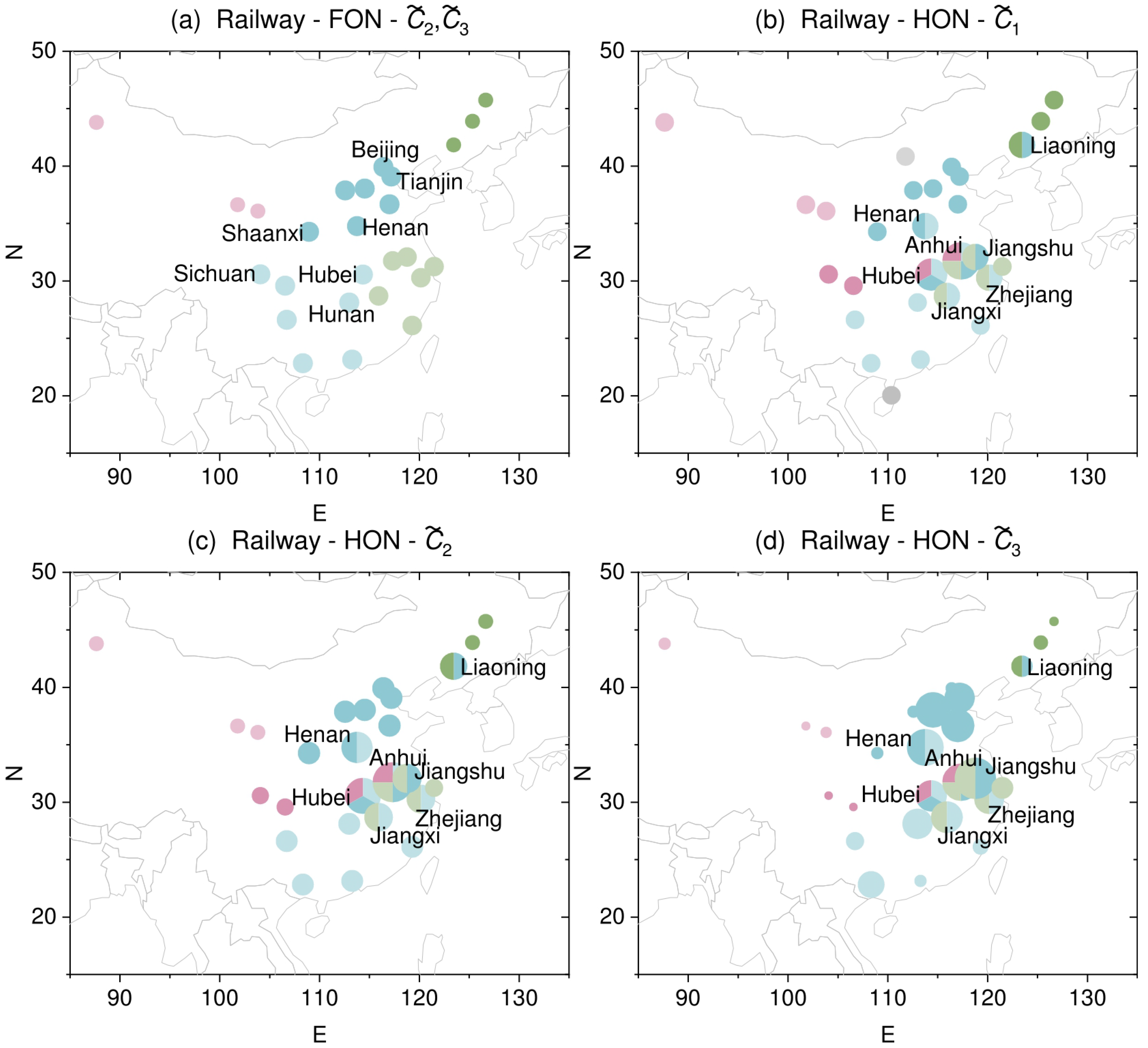
3.3. Results in Railway Flow Dataset

According to the railway flow dataset in 2016, there are a total of 672 stations across 34 provinces (autonomous regions, municipalities, or special administrative regions) in China. Based on location, community, and complexity of these stations or provinces, their roles can be reflected in Chinese railway traffic.

Based on the railway flow dataset, first- and higher-order railway networks are built by the BuildHON+ model. The province communities detected using the Infomap algorithm in the railway network are shown in Figure 5. There are five communities without community overlap in first-order networks; however, there are six or eight communities with community overlap in higher-order networks, where the size of nodes is directly proportional to their complexity.

Based on the location and complexity of provinces in first-order networks as shown in

Table 5. The top 10 provinces with high complexity in railway networks. $n_c$ denotes the number of communities to which a physical node belongs.

Railway—FON			Railway—HON
Province	${\tilde{\mathit{C}}}_{\mathbf{2}},{\tilde{\mathit{C}}}_{\mathbf{3}}$	Edge Province	Province	${\tilde{\mathit{C}}}_{\mathbf{1}}$	${\tilde{\mathit{C}}}_{\mathbf{2}}$	${\tilde{\mathit{C}}}_{\mathbf{3}}$	${\mathit{n}}_{\mathit{c}}$
Hubei	0.845	√	Anhui	4	3.342	18.1	4
Sichuan	0.845	√	Hubei	3	2.643	12.848	3
Hunan	0.845	√	Henan	2	2.041	17.415	2
Tianjin	0.845	√	Jiangxi	2	1.699	13.255	2
Beijing	0.845	√	Zhejiang	2	1.699	11.791	2
Henan	0.845	√	Jiangshu	2	1.74	21.974	2
Shaanxi	0.845	√	Liaoning	2	1.519	5.901	2
Guangdong	0.845	×	Hebei	1	1.041	16.222	1
Guangxi	0.845	×	Shandong	1	1.041	14.414	1
Chongqing	0.845	×	Tianjin	1	1.041	12.075	1

, the hub provinces of the top 7 are Hubei, Sichuan, Hunan, Tianjin, Beijing, Henan, and Shaanxi. Based on the community and complexity of provinces in higher-order networks, the hub provinces of the top 7 are Anhui, Hubei, Henan, Jiangxi, Zhejiang, Jiangsu, and Liaoning. There is more railway traffic in Southeast China, so there should be more hub provinces [23,24]. In higher-order networks, Anhui, Jiangxi, Zhejiang, and Jiangsu, all located in Southeast China, belong to the hub provinces. Meanwhile, in first-order networks, there is no province belonging to the hub provinces. This shows that the above three complexity metrics in higher-order networks perform better than they do in first-order networks. Furthermore, through the observation of higher-order railway networks, the integration of Chinese railway traffic will be deepened by adding high-speed train numbers between Gansu and Shaanxi provinces [25,26].

The station communities detected using the Infomap algorithm in railway networks are shown in Figure 6, where the larger the node, the more complex it is. It is clear that the stations in Southeast China have a larger size overall in higher-order networks than in first-order networks. That is to say, the above three complexity metrics perform better in higher-order networks than they do in first-order networks. Additionally, the higher-order network clearly reveals the Beijing–Guangzhou line, the most important north–south railway artery in China, but the first-order network does not.

3.4. Results in Citation Flow Dataset

The citation flow dataset includes a total of 20 journals, where PRL, PRX, RMP, PRB, PRM, and PRR all belong to multidisciplinary journals [27,28], as shown in

Table 6. The categories of journals reported in JCR in 2020. n denotes the number of papers per journal.

Journal	Category 1	Category 2	Category 3
PRL	Physics, Multidisciplinary	-	-
PRX	Physics, Multidisciplinary	-	-
RMP	Physics, Multidisciplinary	-	-
PRA	Optics	Physics, Atomic, Molecular, and Chemical	-
PRB	Materials Science, Multidisciplinary	Physics, Condensed Matter	Physics, Applied
PRC	Physics, Nuclear	-	-
PRD	Physics, Particles, and Fields	Astronomy, and Astrophysics	-
PRE	Physics, Fluids, and Plasmas	Physics, Mathematical	-
PRAB	Physics, Nuclear	Physics, Particles, and Fields	-
PRAP	Physics, Applied	-	-
PRF	Physics, Fluids, and Plasmas	-	-
PRM	Materials Science, Multidisciplinary	-	-
PRPER	Education, and Educational Research	Education, Scientific Disciplines	-
PRXQ	Quantum Science, and Technology	Physics, Multidisciplinary	Physics, Applied
PRR	Physics, Multidisciplinary	-	-

. Notably, PRL, PRX, and RMP, as the oldest multidisciplinary journals, cover the full range of applied, fundamental, and interdisciplinary physics research topics [29].

Based on the citation flow dataset, first- and higher-order citation networks are built by the BuildHON+ model. Firstly, in Figure 7, node complexity is more distinguishable in higher-order networks than in first-order networks on the whole. For PRL, although it always has the highest complexity in citation networks, there are also differences. ${\tilde{C}}_1$ of PRL is the only highest one in higher-order networks, but there are 20 highest ones in first-order networks; ${\tilde{C}}_2$ of PRL belongs to one of the four highest, but there are eight highest ones in first-order networks; ${\tilde{C}}_3$ of PRL belongs to one of the three highest, but there are eight highest ones in first-order networks. In addition, the complexity of RMP in higher-order networks is higher than that in first-order networks. ${\tilde{C}}_1$ of RMP belongs the top 4 in higher-order networks, but the top 20 in first-order networks; ${\tilde{C}}_2,{\tilde{C}}_3$ of RMP belongs the top 4 in higher-order networks, but the top 8 in first-order networks. Moreover, PRX also has a high level of complexity.

4. Discussions

In addition to the complexity metrics discussed above, the second-order self-citation rate is also a useful metric for evaluating the complexity of specialized journals. When a random walker takes two steps from a node back to the original node in a complex network, the node has one second-order self-citation. Denote specialized journals as the source nodes, and multidisciplinary journals as the bridge nodes. Given the bridge node y, we define the second-order self-citation rate $p_{x\to y\to x}$ in first-order networks as:

$$p_{x\to y\to x}=p_{y\to x}={\displaystyle \frac{w_{y\to x}}{{\sum }_z{w}_{y\to z}}},$$

(12)

where $w_{y\to z}$ denotes the weight of edge $y\to z$, and x and z represent the source node and the target node, respectively.

To eliminate the effects of paper counts per journal, we propose the modified second-order self-citation rate $p_{x\to y\to x}^{+}$ in first-order networks:

$$p_{x\to y\to x}^{+}={\displaystyle \frac{w_{y\to x}/w_x}{{\sum }_z{w}_{y\to z}/w_z}},$$

(13)

where $w_x$ denotes the weight of node x.

Similarly, the modified second-order second-order self-citation rate ${\tilde{p}}_{x\to y\to x}^{+}$ in second-order networks is defined as:

$${\tilde{p}}_{x\to y\to x}^{+}={\displaystyle \frac{w_{y|x\to x}/w_x}{{\sum }_z{w}_{y|z\to x}/w_z}}.$$

(14)

The results have demonstrated the high complexity of PRL, PRX, and RMP, making them suitable as the multidisciplinary journals. Meanwhile, the paper counts of PRA, PRB, PRC, PRD, and PRE are large, making them appropriate as the specialized journals.

As shown in Figure 8, second-order networks are more effective for revealing second-order self-citation than first-order networks, as demonstrated by a comparison of the two second-order self-citation rates. Moreover, the modified second-order second-order self-citation rate of PRB is consistently the highest in second-order networks, which is consistent with the finding in Table 6 that PRB has the most categories. However, that of PRB is the second highest in first-order networks when RMP acts as a bridge node. This suggests that the modified second-order second-order self-citation rate performs better in higher-order networks.

5. Conclusions and Prospects

This paper proposes three quantitative complexity metrics for nodes in higher-order networks using the Infomap algorithm. First, a higher-order network is built by the BuildHON+ model based on flow data. Then, communities are detected using the Infomap algorithm. The complexity metrics are defined as follows: ${\tilde{C}}_1$ of a physical node is the number of communities to which it belongs; ${\tilde{C}}_2$ of a physical node is defined by the number and size of communities to which it belongs; ${\tilde{C}}_3$ of a physical node is defined by the number and size of communities to which it belongs, and the number of higher-order nodes it contains within the same community. Experiments in the Enron flow dataset demonstrate that the proposed complexity metrics identify complex staff more accurately in higher-order networks than in first-order networks. Based on the railway flow dataset, the metrics more accurately identify complex provinces or stations in higher-order networks than in first-order networks. Furthermore, community detection in higher-order networks using the Infomap algorithm reveals the Beijing–Guangzhou line, the most important north–south railway artery in China. In the citation flow dataset, the metrics more accurately identify multidisciplinary journals in higher-order networks than in first-order networks. Additionally, a modified second-order second-order self-citation rate is proposed for second-order networks, which successfully identifies the most complex specialized journals.

This paper defines node complexity from the perspective of community detection using the Infomap algorithm. The next step could involve an in-depth study of how different community-detection algorithms impact node complexity and the resulting outcomes [30]. Additionally, beyond defining node complexity from the community-detection perspective, one could also consider the local or global characteristics of nodes [31]. For instance, degree is the simplest local characteristic [32], while eigenvector is a classical global characteristic [33]. In recent years, the study of flow data within multilayer networks has gained significant attention [9,34], particularly in analyzing human or biological movement trajectories [35,36], where substantial progress has been made. Building on the findings of this paper, the next step could involve integrating the complex structures of multilayer networks with the dynamic characteristics of flow data to propose new node complexity metrics. This research prospect will provide new theoretical tools for multilayer network analysis and contribute to further expanding its applications in biological networks, social networks, and transportation networks, offering new perspectives and methods for the development of related fields.

References

1. Roblek, V.; Dimovski, V. Essentials of ‘the Great Reset’ through Complexity Matching. Systems 2024, 12, 182. [Google Scholar] [CrossRef]
2. Bila, J. Emergent Phenomena in Complex Systems. In Proceedings of the Recent Advances in Soft Computing, Brno, Czech Republic, 20–22 June 2017; Springer: Berlin/Heidelberg, Germany, 2019; pp. 262–270. [Google Scholar]
3. Vargas, D.L. Quantum complexity: Quantum mutual information, complex networks, and emergent phenomena in quantum cellular automata. In Theory of Computing Systems Mathematical Systems Theory; Colorado School of Mines: Golden, CO, USA, 2016; p. 7. [Google Scholar]
4. McShea, D.W. Metazoan complexity and evolution: Is there a trend? Evolution 1995, 50, 477–492. [Google Scholar]
5. Adami, C.; Cerf, N.J. Physical complexity of symbolic sequences. Physica D 2000, 137, 62–69. [Google Scholar] [CrossRef]
6. Fu, Y.; Zhu, J.; Li, X.; Han, X.; Tan, W.; Huangpeng, Q.; Duan, X. Research on Group Behavior Modeling and Individual Interaction Modes with Informed Leaders. Mathematics 2024, 12, 1160. [Google Scholar] [CrossRef]
7. Ahn, Y.Y.; Bagrow, J.P.; Lehmann, S. Link communities reveal multiscale complexity in networks. Nature 2009, 466, 761–764. [Google Scholar] [CrossRef] [PubMed]
8. Benson, A.R.; Gleich, D.F.; Leskovec, J. Higher-order organization of complex networks. Science 2016, 353, 163–166. [Google Scholar] [CrossRef]
9. Scholtes, I. When is a network a network? multi-order graphical model selection in pathways and temporal networks. In Proceedings of the 23rd ACM SIGKDD International Conference on Knowledge Discovery and Data Mining, Halifax, NS, Canada, 13–17 August 2017; pp. 1037–1046. [Google Scholar]
10. Battiston, F.; Cencetti, G.; Lacopini, L.; Latora, V.; Lucas, M.; Patania, A.; Young, J.; Petri, G. Networks beyond pairwise interactions: Structure and dynamics. Phys. Rep. 2020, 874, 1–92. [Google Scholar] [CrossRef]
11. Shi, D.; Chen, G. Simplicial networks: A powerful tool for characterizing higher-order interactions. Natl. Sci. Rev. 2022, 9, nwac038. [Google Scholar] [CrossRef] [PubMed]
12. Li, J.; Lu, X. Measuring the Significance of Higher-Order Dependency in Networks. New J. Phys. 2024, 26, 033032. [Google Scholar] [CrossRef]
13. Gong, C.; Li, J.; Qian, L.; Li, S.; Yang, Z.; Yang, K. HMSL: Source localization based on higher-order Markov propagation. Chaos Solitons Fractals 2024, 182, 114765. [Google Scholar] [CrossRef]
14. Qian, L.; Dou, Y.; Gong, C.; Xu, X.; Tan, Y. Research on User Behavior Based on Higher-Order Dependency Network. Entropy 2023, 25, 1120. [Google Scholar] [CrossRef] [PubMed]
15. Rosvall, M.; Esquivel, A.V.; Lancichinetti, A.; West, J.D.; Lambiotte, R. Memory in network flows and its effects on spreading dynamics and community detection. Nat. Commun. 2014, 5, 4630. [Google Scholar] [CrossRef] [PubMed]
16. Xu, J.; Wickramarathne, T.L.; Chawla, N.V. Representing higher order dependencies in networks. Sci. Adv. 2016, 2, e1600028. [Google Scholar] [CrossRef]
17. Saebi, M.; Xu, J.; Kaplan, L.M.; Ribeiro, B.; Chawla, N.V. Efficient modeling of higher-order dependencies in networks: From algorithm to application for anomaly detection. EPJ Data Sci. 2020, 9, 15. [Google Scholar] [CrossRef]
18. Fu, Y.; Li, X.; Li, J.; Yu, M.; Lu, X.; Huangpeng, Q.; Duan, X. Multi-Scale Higher-Order Dependencies (MSHOD): Higher-Order Interactions Mining and Key Nodes Identification for Global Liner Shipping Network. J. Mar. Sci. Eng. 2024, 12, 1305. [Google Scholar] [CrossRef]
19. Santos, G.G.; Lakhotia, K.; Rose, C.A.F.D. Towards a Scalable Parallel Infomap Algorithm for Community Detection. In Proceedings of the 2024 32nd Euromicro International Conference on Parallel, Distributed and Network-Based Processing (PDP), Dublin, Ireland, 20–22 March 2024; pp. 116–123. [Google Scholar]
20. Velden, T.; Yan, S.; Lagoze, C. Mapping the cognitive structure of astrophysics by infomap clustering of the citation network and topic affinity analysis. Scientometrics 2017, 111, 1033–1051. [Google Scholar] [CrossRef]
21. Li, X.; Zhang, X.; Huangpeng, Q.; Zhao, C.; Duan, X. Event detection in temporal social networks using a higher-order network model. Chaos 2021, 31, 113144. [Google Scholar] [CrossRef]
22. Li, X.; Zhao, C.; Hu, Z.; Yu, C.; Duan, X. Revealing the character of journals in higher-order citation networks. Scientometrics 2022, 127, 6315–6338. [Google Scholar] [CrossRef]
23. Yang, J.; Guo, A.; Li, X.; Huang, T. Study of the Impact of a High-Speed Railway Opening on China’s Accessibility Pattern and Spatial Equality. Sustainability 2018, 10, 2943. [Google Scholar] [CrossRef]
24. Zhu, T.; Xu, Y.; Zhang, J.; Zhao, B. A Bilevel Programming Model for Designing a Collaborative Network for Regional Railway Transportation and Logistics: The Case of the Beijing-Tianjin-Hebei Region in China. J. Adv. Transp. 2024, 2024, 8905446. [Google Scholar] [CrossRef]
25. Ding, S.; Zhang, T.; Sheng, K.; Chen, Y.; Yuan, Z. Key technologies and applications of intelligent dispatching command for high-speed railway in China. Railw. Sci. 2023, 2, 336–346. [Google Scholar] [CrossRef]
26. Hu, W.; Dong, J.; Ren, R.; Chen, Z. Underground logistics systems: Development overview and new prospects in China. Front. Eng. Manag. 2023, 10, 354–359. [Google Scholar] [CrossRef]
27. Wang, X.; Feng, X. Research on the relationships between discourse leading indicators and citations: Perspectives from altmetrics indicators of international multidisciplinary academic journals. Libr. Tech 2022, 42, 1165–1190. [Google Scholar] [CrossRef]
28. Solomon, G.E.A.; Carley, S.F.; Porter, A.L. How Multidisciplinary Are the Multidisciplinary Journals Science and Nature? PLoS ONE 2016, 11, e0152637. [Google Scholar] [CrossRef] [PubMed]
29. Njegovanović, A. Complex Systems in Interdisciplinary Interaction. Financ. Mark. Institutions Risks 2024, 8, 94–107. [Google Scholar] [CrossRef]
30. Huang, X.; Chen, D.; Ren, T.; Wang, D. A survey of community detection methods in multilayer networks. Data Min. Knowl. Discov. 2020, 35, 1–45. [Google Scholar] [CrossRef]
31. Lü, L.; Chen, D.; Ren, X.; Zhang, Q.; Zhang, Y.; Zhou, T. Vital nodes identification in complex networks. Phys. Rep. 2016, 650, 1–63. [Google Scholar] [CrossRef]
32. Liang, J.; Ding, R.; Ma, X.; Peng, L.; Wang, K.; Xiao, W. The Carbon Emission Reduction Effect and Spatio-Temporal Heterogeneity of the Science and Technology Finance Network: The Combined Perspective of Complex Network Analysis and Econometric Models. Systems 2024, 12, 110. [Google Scholar] [CrossRef]
33. Antoine, J.P.; Trapani, C. Operators in Rigged Hilbert Spaces, Gel’fand Bases and Generalized Eigenvalues. Mathematics 2022, 11, 195. [Google Scholar] [CrossRef]
34. Lambiotte, R.; Rosvall, M.; Scholtes, I. From networks to optimal higher-order models of complex systems. Nat. Phys. 2019, 15, 313–320. [Google Scholar] [CrossRef]
35. Fu, Y.; Duan, X.; Li, X.; Han, X.; Deng, J.; Huangpeng, Q. Flocking Modeling and Robustness Evaluation Based on Heterogeneous Network. In Proceedings of the 2024 36th Chinese Control and Decision Conference (CCDC), Xi’an, China, 25–27 May 2024; pp. 1870–1875. [Google Scholar]
36. Gu, K.; Yan, L.; Li, X.; Duan, X.; Liang, J. Change point detection in multi-agent systems based on higher-order features. Chaos 2022, 32, 111102. [Google Scholar] [CrossRef] [PubMed]
Figure 1. The comparison of first- and higher-order network models.
Systems 12 00347 g001
Figure 2. The node complexity-quantification process.
Systems 12 00347 g002
Figure 3. The number of ordinary employees, middle-level managers, and senior leaders occupied in the top 50 nodes ranked by three complexity metrics in Enron networks. (ac) The results ranked by C ˜ 1 , C ˜ 2 , C ˜ 3 in first-order networks, respectively. (df) Those in higher-order networks, respectively.
Systems 12 00347 g003
Figure 4. The sum of complexity grades in the top 50 nodes ranked by three complexity metrics in first- and higher-order Enron networks. (ac) The results ranked by C ˜ 1 , C ˜ 2 , C ˜ 3 in Enron networks, respectively.
Systems 12 00347 g004
Figure 5. The province communities detected using the Infomap algorithm in railway networks. The different colors of the nodes represent their belonging to different communities. (a) The results in first-order networks, where the size of nodes is directly proportional to C ˜ 2 , C ˜ 3 . (bd) The results in higher-order networks, where the size of nodes is in direct proportion to C ˜ 1 , C ˜ 2 , C ˜ 3 , respectively. In addition, E is the east longitude, and N denotes the northern latitude. These parameters are the same with Figure 6. It is important to note that the two figures are both created by ‘Origin 2023’.
Systems 12 00347 g005
Figure 6. The station communities detected using the Infomap algorithm in railway networks.
Systems 12 00347 g006
Figure 7. The complexity calculated by C ˜ 1 , C ˜ 2 , C ˜ 3 in citation networks, respectively. (a) The number of papers per journal. (bd) The complexity comparison of first- and higher-order networks.
Systems 12 00347 g007
Figure 8. The citation flow among five specialized journals via three multidisciplinary journals.
Systems 12 00347 g008