An Improved Driving Safety Field Model Based on Vehicle Movement Uncertainty for Highway Ramp Influence Areas

Abstract

Road traffic accidents result in numerous fatalities and injuries annually. Advanced driving assistance systems (ADASs) have garnered significant attention to mitigate these harms. An accurate safety assessment can significantly improve the effectiveness and credibility of ADASs. However, a real-time safety assessment remains a key challenge due to the complex interactions among humans, vehicles, and the road environment. Traditional safety assessment methods, relying on crash data and surrogate safety measures (SSMs), face limitations in real-time applicability and scenario coverage, especially in freeway ramp areas with frequent merging and lane changing. To address these gaps, this paper develops a driving safety field based on the uncertainty of vehicle movements, which integrates the characteristics of driving behaviors, vehicles, and the road environment. The proposed method is validated with a simulation of driving scenarios and ROC curves obtained from the NGSIM dataset. The results demonstrate that our proposed driving safety field effectively quantifies the real-time risk in ramp influence areas and outperforms Time to Collision (TTC), making it suitable for integration into collision warning systems of ADASs.

1. Introduction

According to data from the World Health Organization in 2023, road traffic accidents cause the deaths of approximately 1.19 million people each year, and the number of people suffering non-fatal injuries ranges from 20 million to 50 million [1]. To mitigate the harm caused by traffic accidents, advanced driving assistance systems (ADASs) have received extensive attention [2]. However, a fundamental problem in designing ADASs is the real-time assessment of safety. Considering that the traffic system is a complex system involving intricate interactions among humans, vehicles, and the road environment [3,4], it is challenging to accurately assess real-time traffic safety under different road environments and driving styles.

Safety is considered a subjective perception of road users [5]. To find a general representation of road safety, it is necessary to replace this perception with ground truth data that can be directly obtained in road traffic. Currently, safety assessment methods based on crash data (including frequency and severity) [6] and surrogate safety measures (SSMs) are the most extensively applied [7]. However, these methods have limitations in terms of their real-time applicability and scope of scenarios [8]. Specifically, crash-based methods, while able to account for the impact of external factors such as road characteristics on traffic safety, cannot perform real-time assessments. Conversely, SSM-based methods can provide real-time evaluations but rely on strong assumptions about vehicle motion patterns, which limits their applicability to complex scenarios [9].

In designing driver assistance systems, a SSM is always considered the criterion for risky events because crash-based measures cannot be obtained in real time [10]. However, there are still gaps in real-time safety assessments for complex traffic scenarios [11]. The movement of vehicles has uncertainty, and this uncertainty violates the basic assumptions of SSMs. Therefore, it is necessary to incorporate more information on the traffic systems to eliminate this uncertainty. Extensive relevant research has been carried out, especially about the characteristics of drivers. Currently, the driving style can be recognized in real time [12,13,14] and integrated into the design of ADASs [15]. However, the characteristics of the road environment have obtained limited attention, which may bring about flaws in ADASs in different road types. The dynamics of vehicles in different road types differ obviously, necessitating the incorporation of the road environments characteristic. Especially in freeway ramp areas, the traffic flow characteristics are more complex, with frequent merging and lane changing. Due to the necessity for vehicles to enter and exit ramps, traffic conflicts and accidents are frequent [16]. The weaving risk in these areas significantly differs from normal driving conditions on other road sections. Existing SSM-based methods often underestimate the collision risk posed by adjacent lane vehicles, while accident-based safety assessment methods are lagging and struggle to capture dangerous vehicle interactions in real time. Although some field-based safety assessment approaches have also been proposed to integrate lateral kinematics, they ignore the difference of driving behaviors in different road environments. And the difficulty in parameters’ calibration fails in its further application in these scenarios [17,18,19,20].

To address these research gaps, this paper aims to construct a more comprehensive safety measure theory that (1) has strong physical significance and reflects a full range of collision patterns and (2) incorporates road attributes (such as ramps or weaving areas) and vehicle attributes. The remainder of this paper is organized as follows: Firstly, we conducted a comprehensive literature review in Section 2. In Section 3, we provide a brief introduction to the data we selected (the US-101 segment from NGSIM), along with a description of data processing and ramp area selection criteria. Section 4 presents the methodology for constructing the driving risk field in the ramp area. In Section 5, we validate the proposed methodology using ROC curves and simulation in driving scenarios. Then, we compare it with the widely used Time to Collision method. The conclusion, limitations, and directions for further study are discussed in Section 6.

2. Literature Review

2.1. Safety Evaluation Based on Crash Data

Crash data are most commonly used in traditional theories of safety estimation, utilizing frequency to estimate probability. Traffic safety assessment theories based on accident data are summarized as a direct traffic safety analysis. Typical inputs for these models include road traffic accident rates [21] (often measured in accidents per million vehicle kilometers) and the severity levels of road accidents. This approach primarily involves establishing generalized regression models, such as Poisson regression models [22], negative binomial regression models [23], and Poisson-lognormal models [20], or designing before-and-after control experiments [24] to explore the relationships between accident frequency, severity, and related factors.

For example, Alarifi et al. [25] developed a multivariate hierarchical Poisson-lognormal model to estimate six different collision types at signalized intersections (same direction, angle, and turning collisions, opposite direction, non-motorized, multi-vehicle, and single-vehicle collisions). Their study indicated correlations between most types of collision counts, with a significant negative correlation between left-turn collision frequency and left-turn phase duration. Bauer and Harwood [26] used a negative binomial regression model to establish a statistical relationship between ramp traffic accidents and factors like traffic volume and road geometry design.

However, a direct traffic safety analysis faces inherent challenges due to the endogenous differences within experimental control and treatment groups, as well as the high amount of collision data required. These challenges include the following: (1) traffic accidents are sparse events [27], leading to small sample sizes [28], which may cause analytical heterogeneity; (2) historical accident data cannot be used for a real-time or advanced analysis [29]; and (3) minor accidents and property damage-only accidents are often not recorded in accident reports [30], leading to the neglect of some hazardous situations. Therefore, the assessment method based on crash data is difficult to apply to a real-time safety assessment, especially in the design of ADASs. In order to overcome the inherent limitations of the direct traffic safety analysis method, safety-critical events are relaxed to conflicts, since these conflicts are more common and easier to obtain. These conflicts are considered as the transition of normal events and crashes. Some real-time crash-forecasting models based on deep learning have been proposed, and are currently based on conflicts data instead of crash data. Islam and Abdel-Aty [31] applied long-short term memory (LSTM) based on connected vehicle data (mainly including GPS location, heading, speed, and postal code). Orsini et al. [32] proposed a real-time conflict prediction model (RTConfPM), which can identify potential conflicts with radar data by the support vector machine and extreme value theory. However, these approaches may not be available in the design of ADASs currently. The main obstacles can be divided into two aspects: (1) the deep-learning or machine-learning-based methods need offline pre-training, causing defects in transferability and accuracy in practical application [31] and (2) the deep-learning methods are black box ones; the direct physical significance and interpretability need to be enhanced [33].

2.2. Surrogate Safety Measures

Considering the requirement of objectivity and availability, indirect traffic safety assessment methods are widely used today. The core idea of indirect traffic safety assessment is to use non-accident data as the dependent variable in the model instead of accident data. The most widely applied technique in indirect traffic safety assessments is surrogate safety measures (SSMs). The principle behind SSMs is that safety-critical events occur more frequently than collisions, and they can be revealed through indicators of vehicle interactions [34]. Traditional SSMs include Time to Collision (TTC) [35], Aggregated Time to Collision [36], Post-Encroachment Time (PET) [37], and the Deceleration to Safety Time Index (DSTI) [38]. A detailed review of surrogate safety measures can be found in the work by Wang et al. [39]. These SSMs have been applied extensively in the design of ADASs. For example, the Time to Collision method is commonly used as the basis of forward collision systems [40]. However, most SSMs only consider the sole pattern of potential collision, and they have an inability when dealing with complex driving scenarios. Freedy et al. argued [41] that most current SSMs (like TTC and PICUD) will cause false positive warnings when vehicles in different lanes are involved. To better capture two-dimensional conflicts, some field theory-based SSMs have also been proposed.

Field theory is derived from the obstacle avoidance of robots [42]. The involved entities are modeled as point charges in the electric field. There exists a repulsive force between the entities, and the robots can avoid the avoidance along the gradient descent direction of the potential field. Ni et al. [43] firstly introduced field theory into traffic flow to model the lane-changing behaviors. Currently, field theory has been applied in the road safety evaluation and design of ADASs extensively. Wang et al. initially proposed the concept of a driving safety field (DSF), using potential energy to quantify safety levels [17]. Based on the driving safety field, the design of the forward collision warning system (FCW) can be enhanced, especially when dealing with muti-lane scenarios. Similarly, Li et al. [18] utilized the safety potential field (SPF) model to improve the framework of model predictive control (MPC). The improved framework can increase the traffic capacity by about 24.4%. Arun et al. [44] claim the potential energy of the safety field outperforms other traditional SSMs in safety assessments and extreme value modeling. Besides the field based on potential energy, there also exists a field based on probability and risk perception. Freedy et al. introduced a probabilistic field approach that, by incorporating the uncertainties of neighboring vehicle movements, calculated the probability of a vehicle being involved in an accident within a given time frame [19]. This method can more comprehensively reflect different collision patterns (such as rear-end and side collisions). Kolekar constructed the driver’s risk field (DRF), which is a two-dimensional field representing the belief of drivers [20]. Generally, these safety assessment methods based on safety measures are relatively effective in most traffic scenarios. Because they can be obtained in real time and with ease, driving assistance systems (especially collision avoidance systems) based on SSMs have also been widely developed [45].

Nonetheless, existing SSMs are mainly based on the assumption that the driver’s motion state is unchanged, ignoring the uncertainty of the driver’s intentions and behaviors. In complex driving scenarios, the existing SSMs are no longer applicable. Additionally, they overlook the impact of other external factors on safety (such as driver style and road type). Apart from the vehicle’s own dynamic characteristics, external environments [46] and surrounding vehicle characteristics (such as mass and size) [47] also impact the probability and severity of potential accidents [48]. Current studies have not sufficiently addressed these factors, leading to the failure of existing safety measures in accurately estimating real-time risks in complex traffic scenarios, which may result in false positive or false negative alarms [49]. For example, the rules of dynamics in highways may not be applicable in ramps. While it has been ignored in current SSMs (including field-based SSMs), these problems limit the further application of SSMs. Especially in ramp areas with complex road environments, a more accurate and comprehensive risk quantification method is needed.

2.3. Road Safety of Ramp Influence Areas

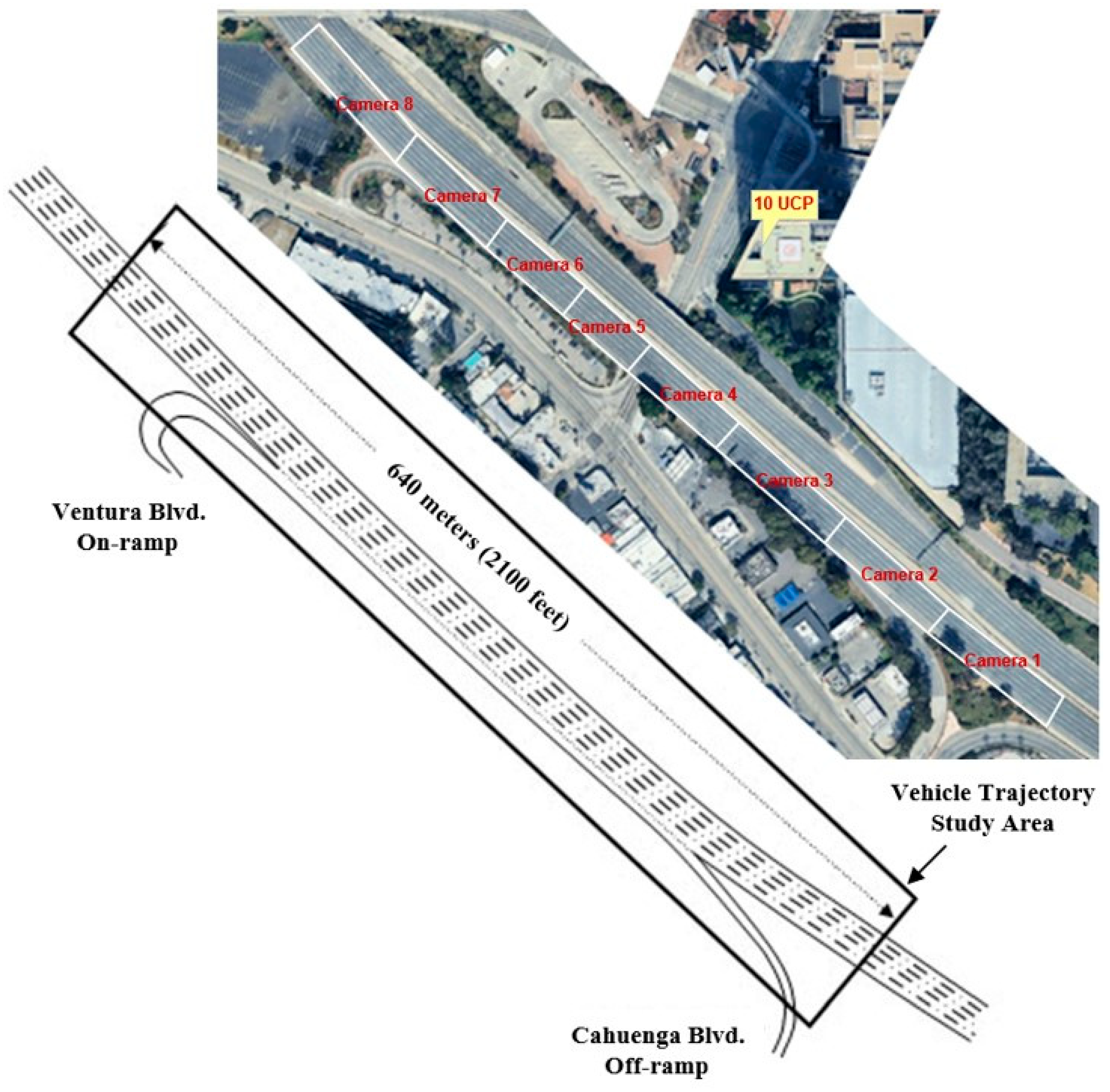
Ramp influence areas are vital zones on freeways where merging and diverging vehicle maneuvers elevate the risk of traffic conflicts and accidents. The restricted space and overlapping zones in these regions generate complex and unstable traffic conditions, increasing their susceptibility to crashes [50]. Several studies have examined the impact of external factors (including geometric design [51], operational measures [52], and traffic flow characteristics [53]) on the safety performance in ramp influence areas. For instance, Zhao et al. [51] employed multilevel logistic regression models to investigate the effects of geometric design variables on crash risk, revealing significant interactions between these variables and traffic conditions. The research indicates that the length of weaving areas will significantly increase the likelihood of a crash. And drivers will have more sudden accelerating and deceleration behaviors in such areas. Zhu et al. found that the driving risk in the ramp influencing areas is higher than the main road [16]. In addition, a significant feature of the ramp influence area is that vehicles have significant lateral behavior. Considering the significant difference in vehicle movement between the main road section and the weaving area, the main collision types on the ramp are sideswipe and angle crashes, rather than rear-end events. However, the current SSM is mainly used to identify the rear-end time, which makes them unable to accurately judge the ramp risk in real time [54]. To override these challenges, more comprehensive risk quantification methods that account for the dynamic nature of driver behavior and external influences are needed. Such methods could enhance the effectiveness of advanced driving assistance systems (ADASs) by providing accurate real-time safety assessments, ultimate reducing the crash risk in ramp influence areas.

3. Data Materials

3.1. Introduction of US-101

This study uses the NGSIM dataset for parameter calibration and validation. The NGSIM dataset was collected by the Federal Highway Administration (FHWA) between 2005 and 2006 to support the research of microscopic vehicle behaviors [55]. The dataset includes high-quality trajectory data collected at four different locations: two freeway segments (I-80 and US-101) and two arterial road segments (Lankershim Boulevard and Peachtree Street). Given that this study focuses on vehicle driving risks in ramp influence areas, there exists no ramp influencing areas in I-80, so we selected vehicle trajectory data collected on US-101 in Los Angeles, CA, USA. A diagram of the study area is shown in Figure 1.

The data collection area is approximately 640 m (2100 feet) long, with five mainline lanes, and an auxiliary lane in the corridor section between the Ventura Boulevard entrance ramp and the Cahuenga Boulevard exit ramp. It includes 45 min of data divided into three 15-min periods including 7:50–8:05 a.m., 8:05–8:20 a.m., and 8:20–8:35 a.m. on 15 June 2005. The frequency of the data is 10 HZ. Although extensive dimensions of the trajectory (including the ID of vehicles, size of vehicles, position, and lane) have been given in the dataset, the velocity and acceleration cannot be obtained directly. Here, we use differentiation to calculate speed and acceleration; the method of calculation can be found in Equations (1)–(4).

$$v_{X,t}={\displaystyle \frac{X_{t+∆t}-X_t}{∆t}}$$

(1)

$$v_{Y,t}={\displaystyle \frac{Y_{t+∆t}-Y_t}{∆t}}$$

(2)

$$a_{X,t}={\displaystyle \frac{v_{X,t+∆t}-v_{X,t}}{∆t}}$$

(3)

$$a_{Y,t}={\displaystyle \frac{v_{Y,t+∆t}-v_{Y,t}}{∆t}}$$

(4)

where $X_t$ denotes the lateral position (lateral direction here refers to the direction perpendicular to the road) at time t, and $X_{t+∆t}$ denotes the lateral position at time $t+∆$t. Similarly, $Y_t$ and $Y_{t+∆t}$ denote the longitudinal position at time t and $t+∆t$. $v_{X,t}$, $v_{Y,t}$, $a_{X,t},$ and $a_{Y,t}$ are the velocity and acceleration obtained after differentiation. $∆t$ is the step of differentiation, which is equal to 0.5 s here. And the diagram of data processing can be found in Figure 2.

Additionally, to reduce the error in the calculated speed and acceleration values, we applied a Savitzky–Golay filter. In this study, we selected a window size of 21, corresponding to 2 s of trajectory data. For each position coordinate, we considered the point and its 10 preceding and 10 succeeding data points (a total of 21 data points) to fit a second-order polynomial. A new estimated value was generated for each data point, based on the polynomial fit of its neighboring data points. This approach reduces the noise in the original data while preserving the main characteristics of the signal, such as peaks and widths.

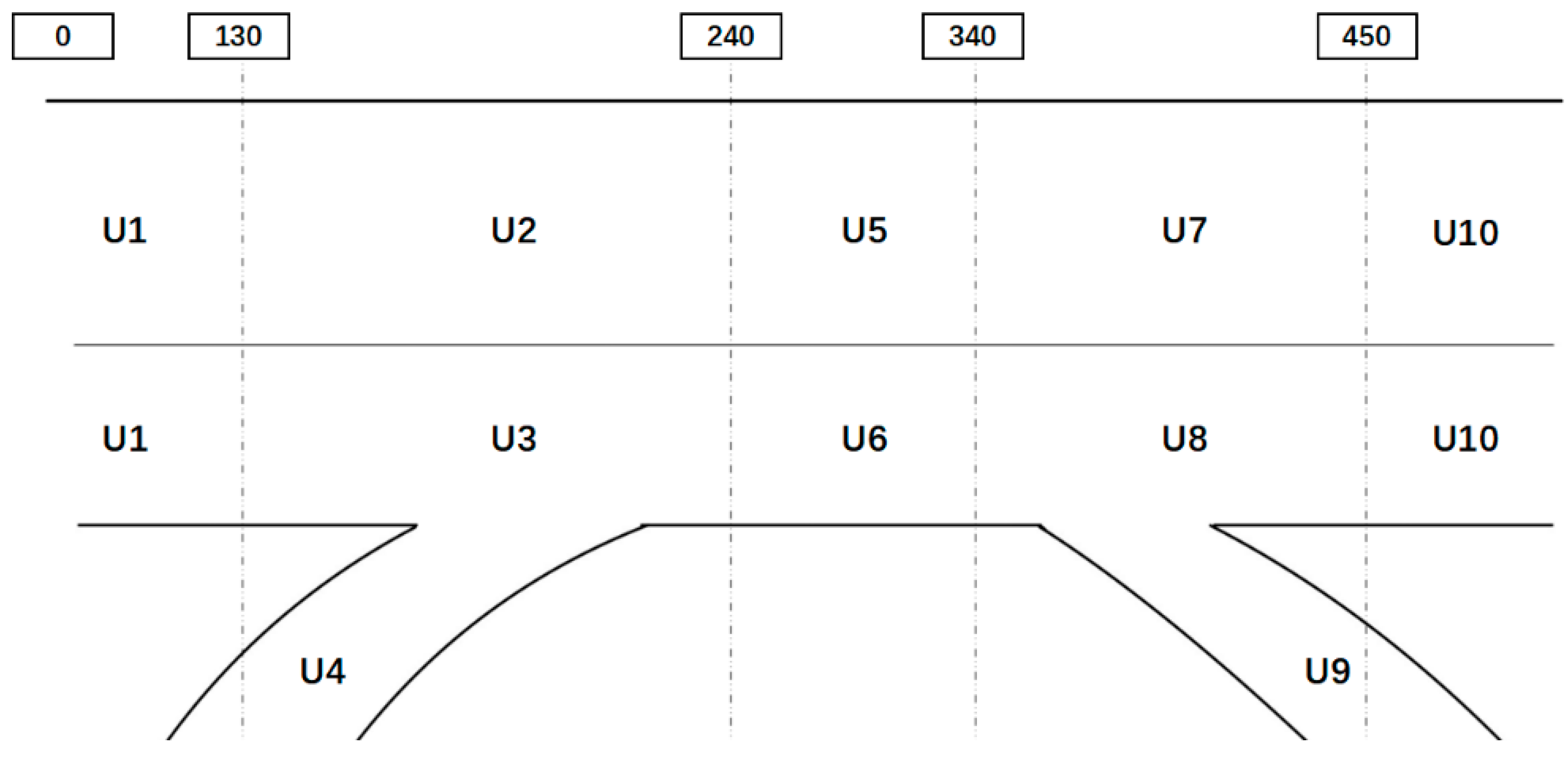
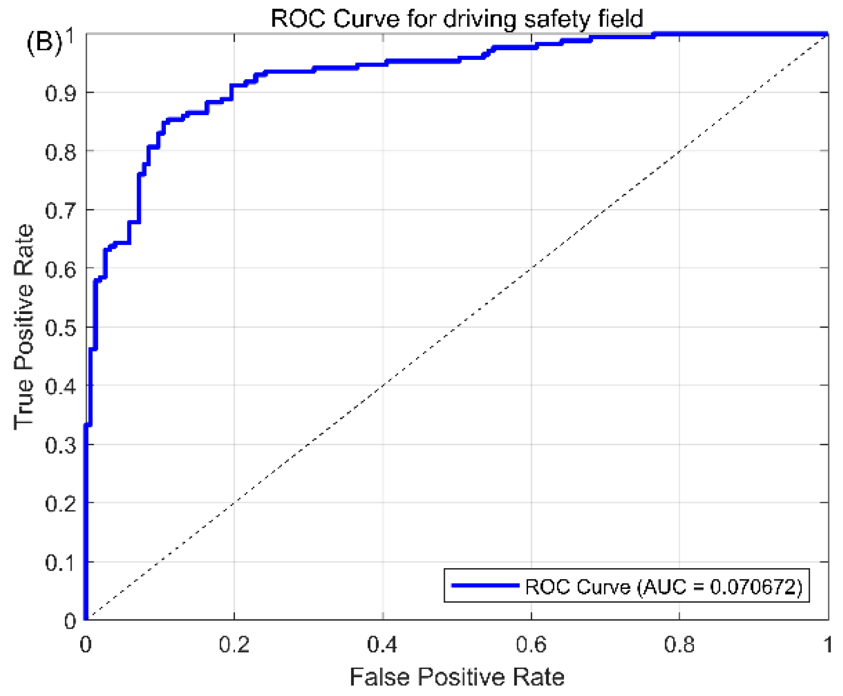
3.2. Ramp Area Segmentation

After the processing in Section 2.1, we obtained the speed and acceleration data from the vehicle trajectories, which more comprehensively reflect the vehicle dynamics characteristics. Using the speed data derived from differentiation, we plotted the trajectory–speed graph for the US-101 dataset, as shown in Figure 3. Based on the shapes of the trajectories, we segmented the road sections, with the segmentation results shown in

Table 1. Segmentation results and corresponding kinematic characteristics.

Longitudinal Position	Segment	Mean (and Var) of Lateral	Mean (and Var) of Longitudinal
0–130	Upstream	0.043 (0.039)	8.428 (10.795)
130–240	Entrance ramp	−0.012 (0.057)	9.155 (14.281)
240–340	Mainline segment	−0.015 (0.032)	9.475 (17.499)
340–450	Exit ramp influence	0.005 (0.032)	10.227 (20.429)
450–700	Downstream	0.015 (0.044)	10.488 (26.051)

.

4. Methodology

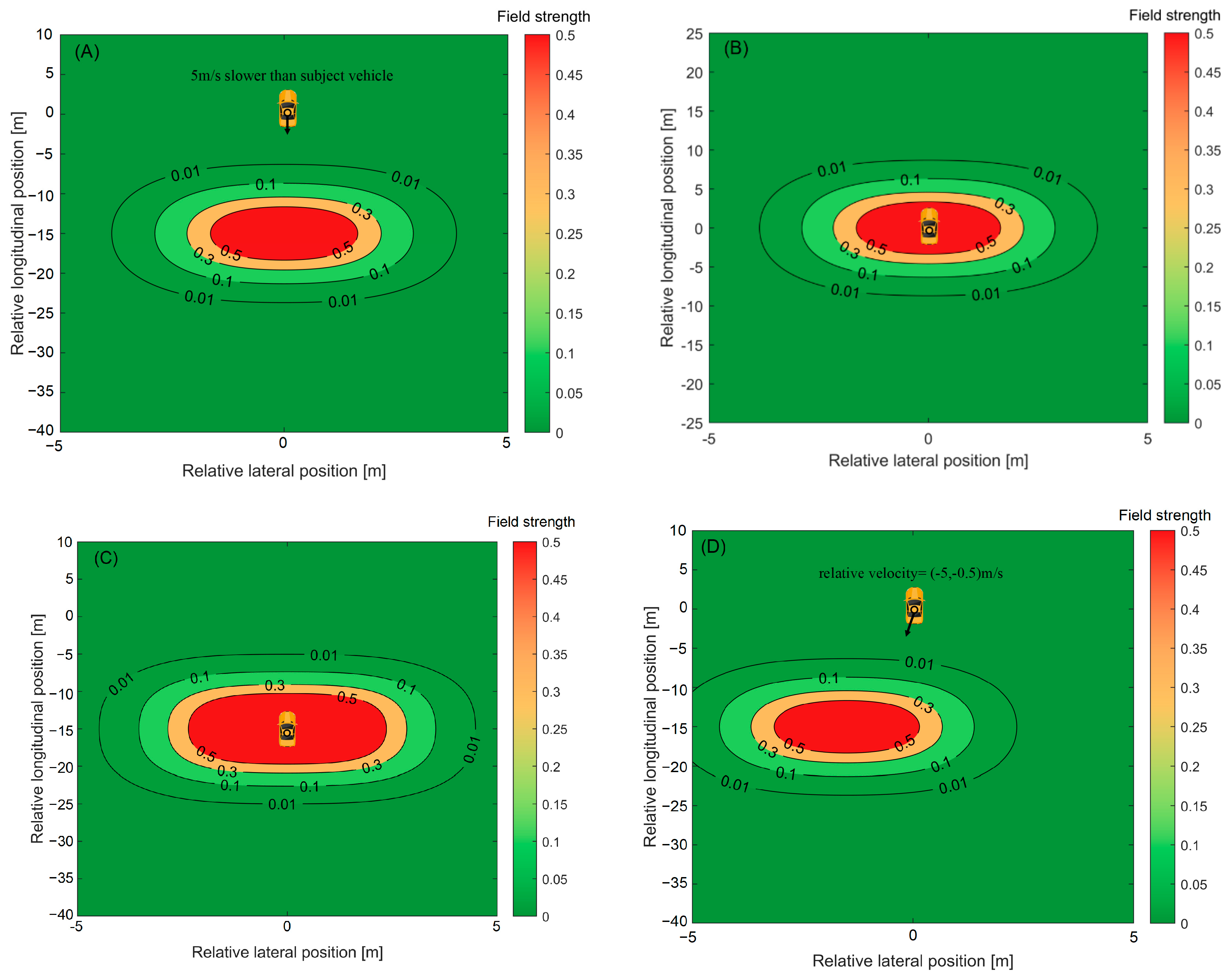
4.1. Construction of Safety Field

To capture collisions of extensive patterns, we apply the concept of field in this work. In typical safety field theories, the subject vehicle is analogous to point charges. Surrounding vehicles exert a repulsive force on the subject vehicle (similar to the interaction force between electric charges). The field strength is a scalar value that changes with position (x, y), describing the real-time safety level of the vehicle. The potential energy and the field strength are always considered the value of safety in most field-based metrics [17,18]. In this research, we will incorporate the uncertainty of kinematics into the SSM and use the probability to represent safety, like in the study by Freedy et al. [19]. The proposed safety field is irrotational and the potential energy is not applicable here. So, we use the safety field strength to represent the degree of safety:

$$S=E(x,y)$$

(5)

In Equation (5), S is the value of safety and E is the strength of safety field. Please note that in Equation (5), the position of the subject vehicle is considered the sole independent variable. This implies that in a given scenario, the vehicle’s risk is uniquely determined by its position. The influence of the road environment (which typically refers to the type of road), surrounding vehicle attribution (including size and mass), and vehicle dynamics (such as speed) on vehicle safety is reflected through these factors being parameters in the calculation of the risk field, as shown in Equation (6):

$$E\left(x,y\right)=E(x,y|R,W,L,V,M)$$

(6)

where $R$ denotes the road environment, W and L represent the types of neighbor vehicles (W refers to width and L refers to the length), V includes the vehicle dynamics characteristics, and M refers the mass of the involved vehicles. The functional form in Equation (6) is not unique. For example, Wang et al. [17] used a negative power function of vehicle distance. To incorporate the vehicle size, road type, and vehicle kinematic indicators into the framework and derive an interpretable functional form, we consider the following idea:

A collision is a probabilistic event, not a deterministic event. This uncertainty arises from the unpredictability of the neighboring vehicle’s movements. For example, when two vehicles are following each other at similar speeds and close distances, a collision will not happen based on their current kinematic states. However, this situation still represents a high-risk event primarily due to the potential deceleration behavior of the leading vehicle. To quantify this operational uncertainty, we consider the probability distribution of the neighboring vehicle’s acceleration $P\left(a\right)$. This is reasonable because a vehicle’s behavior is controlled by changing its acceleration, and the probability distribution of acceleration reflects the vehicle’s behavior distribution, which is related to the type of road $R$.

After obtaining the probability distribution of the neighboring vehicle’s acceleration, we can calculate the collision probability after $∆t$ seconds based on the current vehicle’s position and speed. The position of the subject vehicle after $∆\mathrm{t}$ is S₁.

$$S_1=[X_{s,t+∆t}-{\displaystyle \frac{W_s}{2}},X_{s,t+∆t}+{\displaystyle \frac{W_s}{2}}]\oplus [Y_{s,t+∆t}-{\displaystyle \frac{L_s}{2}},Y_{s,t+∆t}+{\displaystyle \frac{L_s}{2}}]$$

(7)

S₁ is a deterministic set because the driver of the subject vehicle can control their manipulation. The uncertainty derives from the uncertainty of neighbor driver’s manipulation. This uncertainty is reflected by the distribution $P\left(a\right)$; if the neighbor vehicle and S₁ have overlap, the crash will occur. We define the position set of the neighbor vehicle’s geometric center after $∆t$ under the situation of crash as $S_2$, which can be calculated as follows:

$$S_2=[X_{s,t+∆t}-{\displaystyle \frac{W_s+W_n}{2}},X_{s,t+∆t}+{\displaystyle \frac{W_s+W_n}{2}}]\oplus [Y_{s,t+∆t}-{\displaystyle \frac{L_{s+L_n}}{2}},Y_{s,t+∆t}+{\displaystyle \frac{L_{s+L_n}}{2}}]$$

(8)

During this calculation, the vehicle size is naturally embedded, considering that the vehicle size correlates with the conflict position set $S_2$, as the Figure 4 shows. Here, $X_{s,t+∆t}$ and $Y_{s,t+∆t}$ denote the lateral and longitudinal position of the subject vehicle’s geometric center, and $W_s$ and $L_s$ are the width and length of the subject vehicle. $W_n$ and $L_n$ represent the size of the neighbor vehicle. If the position (geometric center) of the neighbor vehicle locates within the conflict set $S_2$, the crash will occur. The position of the subject and neighbor vehicle can be estimated by the following:

$$(X_{s,t+∆t},Y_{s,t+∆t})=(X_{s,t},Y_{s,t})+(V_{s,t}^x,V_{s,t}^y)∆t$$

(9)

$$\left(X_{n,t+∆t},Y_{n,t+∆t}\right)=\left(X_{n,t},Y_{n,t}\right)+\left(V_{n,t}^x,V_{n,t}^y\right)∆t+{\displaystyle \frac{\left(a_{n,t}^x,a_{n,t}^y\right){∆t}^2}{2}}$$

(10)

In Equations (9) and (10), $(V_{s,t}^x,V_{s,t}^y)$ and $(V_{n,t}^x,V_{n,t}^y)$ represent the velocity vector of the subject vehicle and neighbor vehicle, respectively. $(a_{n,t}^x,a_{n,t}^y)$ represents the acceleration vector of the neighbor vehicle, which incorporates the uncertainty of its movement. The crash will occur under some given acceleration of the neighbor vehicle, thus the probability of collision (the geometric center located within S₂) can be calculated by the acceleration distribution of the neighbor vehicle. Based on Equations (7)–(10), the probability of collision can be calculated as follows:

$$\mathrm{P}\left(\left(X_{n,t+∆t},Y_{n,t+∆t}\right)ϵS_2\right)=\underset{S_2\to A}{\iint }P\left(a_{n,t}^x,a_{n,t}^y|R\right)d{a}_{n,t}^{x}d{a}_{n,t}^y$$

(11)

Equation (11) indicates that the acceleration probability distribution is determined by the types of the road (such as ramp and main road). Here, ${\mathrm{S}}_2\to \mathrm{A}$ refers to the rule of mapping from the conflict set to the acceleration set, which is as follows:

$$\begin{array}{c}A=\left\{\left(a_{n,t}^x,a_{n,t}^y\right)|\left(a_{n,t}^x,a_{n,t}^y\right)={\displaystyle \frac{\left(X_{n,t+∆t},Y_{n,t+∆t}\right)-\left(X_{n,t},Y_{n,t}\right)-\left(V_{n,t}^x,V_{n,t}^y\right)∆t}{{0.5∆t}^2}},\left(X_{n,t+∆t},Y_{n,t+∆t}\right)ϵS_2\right\}\end{array}$$

(12)

Equations (11) and (12) provide the probability of collision after $∆\mathrm{t}$; this probability can be considered as the strength of the safety field in Equation (6). According to Equations (6), (11) and (12), the collision probability field can be represented as follows:

$$E\left(x,y\right)=\mathrm{P}\left(\left(X_{n,t+∆t},Y_{n,t+∆t}\right)ϵS_2\left|\left(a_{n,t}^x,a_{n,t}^y|R\right),\left(W_s,W_n\right),\left(L_s,L_n\right),\left(V_{s,t}^x,V_{s,t}^y,V_{n,t}^x,V_{n,t}^y\right),∆t\right)\right)$$

(13)

It should be noted that the severity of collision can also be integrated in this field by introducing the loss kinetic energy in perfectly inelastic collisions [19]. In that case, the following is true:

$$E\left(x,y\right)=\mathrm{P}\left(\left(X_{n,t+∆t},Y_{n,t+∆t}\right)ϵS_2\right){\displaystyle \frac{M_s{M}_n^2}{2{\left(M_s+M_n\right)}^2}}{{‖(V_{s,t}^x,V_{s,t}^y)-(V_{n,t}^x,V_{n,t}^y)‖}_2}^2$$

(14)

Here, $M_s$ and $M_n$ are the mass of the subject vehicle and neighbor vehicle. Considering that the mass of the vehicle is difficult to obtain directly, in this research, we use Equation (13) to determine the strength of the safety field. For example, assuming that the neighboring vehicle is located at the coordinate axis (0 m, 0 m), the longitudinal (y-axis) speed of the subject vehicle is 25 m/s, and there is no lateral speed of the subject vehicles. Additionally, the acceleration of the neighbor vehicle is assumed to obey the normal distribution $N({\mu }_x{,\mu }_y,{\sigma }_x,{\sigma }_y,0)$.

Figure 5 displays the safety field under this condition. Our proposed safety field can depict the level of safety under different conditions. The safety field varies when the following conditions occur: (a): the neighbor vehicle has specific behaviors (like decelerate, see Figure 5A,B), (b): the size of neighbor vehicle changes (see Figure 5A,C), and (c): the neighbor vehicle changes its lane (see Figure 5A,D).

4.2. Gaussian Mixture Model

In Section 4.1, we have discussed that the behavior of the vehicles will be different in different road areas (like main road and ramp). And this characteristic is reflected by the probability distribution of acceleration $f\left(a_{n,t}^x,a_{n,t}^y\right)$. Considering that acceleration indicates the behavior of the vehicles, this behavior varies in different road areas. And each region may have multiple patterns of behaviors. Here, we further discuss this distribution with the Gaussian Mixture Model.

The Gaussian Mixture Model (GMM) extends the single Gaussian Model by linearly combining K Gaussian distributions, and it is characterized by its flexibility, simplicity, and well-fitting performance. It can be expressed as follows:

$$f\left(x\right)=\sum _{i=1}^k{\alpha }_{i}f\left(x|{\mathit{\mu }}_{\mathit{i}},{\mathsf{\Sigma }}_{\mathit{i}}\right)$$

(15)

where $k$ is the dimension of the GMM. Each dimension corresponds to a Gaussian distribution, and the model is the probability density function of the normal distribution when $\mathrm{k}=1$. And ${\mathit{\mu }}_{\mathit{i}}$, ${\mathit{\Sigma }}_{\mathrm{i}}$ is the mean vector and covariance matrix of the Gaussian distribution $\mathrm{i}$, which is used to determine the shape. ${\alpha }_i\in \left(\mathrm{0,1}\right]$ is the mixture coefficient, which can be regarded as the probability of selecting the Gaussian distribution $i$, ${\sum }_i^k{\alpha }_i=1$.

Various methods have been proposed for estimating parameters in GMM, including maximum likelihood (ML), Expectation-Maximization (EM), and Markov Chain Monte Carlo (MCMC), among others. In this study, we chose to employ the EM algorithm for parameter estimation due to its efficiency in handling models with latent variables and its iterative approach, which simplifies complex calculations. The EM algorithm also guarantees convergence, making it a robust choice for our model [56]. The parameters to be estimated are denoted as ${\theta }_i=\left\{{(\alpha }_i,{\mu }_i,{\Sigma }_i\left)\right|i=1,2,\dots ,k\right\}$.

EM is an algorithm to find the maximum likelihood estimate of a parameter in a probabilistic model. The process can be divided into two steps: (1) expectation: if the parameters are known, the expectation of the implicit variables can be calculated and (2) maximization: if the implicit variables are known, the maximum likelihood of the parameters can be estimated. These two steps perform iteratively. Here, we provide the mathematical form of the solution process:

Using a sample set of size $\mathrm{N}$ to estimate all the parameters in the GMM: ${{\Theta =({\theta }_1,{\theta }_2,\dots ,\theta }_k)}^T$. And the log-likelihood function of the sample set can be expressed as follows:

$$L\left(\mathit{X}|\mathsf{\Theta }\right)=\ln \prod _{j=1}^N{f}_k\left({\mathit{X}}_{\mathit{j}}\right)=\sum _{j=1}^N\ln \sum _{i=1}^K{\alpha }_i{f}_i\left({\mathit{X}}_{\mathit{i}}|{\mathit{\mu }}_{\mathit{i}},{\mathsf{\Sigma }}_{\mathit{i}}\right)$$

(16)

Assuming that the initial estimated parameter of the GMM is ${\Theta }^{\left(0\right)}$, and the parameter at the iteration step $\mathrm{q}$ is ${\Theta }^{\left(q\right)}$, the iterative process $(\mathrm{q}+1)$ is as follows:

(1) E-step

Calculate the posterior probability that each sample belongs to the Gaussian distribution $\mathrm{i}$, based on ${\mathsf{\Theta }}^{\left(\mathrm{q}\right)}$:

$${\overline{{\alpha }_{ij}}}^{\left(q+1\right)}={\displaystyle \frac{{{\alpha }_i}^{\left(q\right)}\cdot f_i\left({\mathit{X}}_{\mathit{j}}|{\mathsf{\Theta }}^{\left(\mathit{q}\right)}\right)}{\sum _{l=1}^k{{\alpha }_l}^{\left(q\right)}\cdot f_l\left({\mathit{X}}_{\mathit{j}}|{\mathsf{\Theta }}^{\left(\mathit{q}\right)}\right)}},1\le i\le K,1\le j\le N$$

(17)

(2) M-step

After obtaining the posterior probabilities of each sample, solve (2) using gradient descent to obtain the estimated values.

$${{\alpha }_i}^{\left(q+1\right)}=\sum _{j=1}^N{\overline{{\alpha }_{ij}}}^{\left(q+1\right)}$$

(18)

$${{\mathit{\mu }}_{\mathit{i}}}^{\left(\mathit{q}+1\right)}={\displaystyle \frac{\sum _{j=1}^N{\overline{{\alpha }_{ij}}}^{\left(q+1\right)}{\mathit{X}}_{\mathit{j}}}{\sum _{j=1}^N{\overline{{\alpha }_{ij}}}^{\left(q+1\right)}}}$$

(19)

$${{\sigma }_i}^{\left(q+1\right)}={\displaystyle \frac{\sum _{j=1}^N{\overline{{\alpha }_{ij}}}^{\left(q+1\right)}\left({\mathit{X}}_{\mathit{j}}-{{\mathit{\mu }}_{\mathit{i}}}^{\left(\mathit{q}+1\right)}\right){\left({\mathit{X}}_{\mathit{j}}-{{\mathit{\mu }}_{\mathit{i}}}^{\left(\mathit{q}+1\right)}\right)}^T}{\sum _{j=1}^N{\overline{{\alpha }_{ij}}}^{\left(q+1\right)}}}$$

(20)

Repeat the E-step and M-step until $‖{\mathsf{\Theta }}^{(\mathrm{q}+1)}-{\mathsf{\Theta }}^{\left(\mathrm{q}\right)}‖$ converge, then stop.

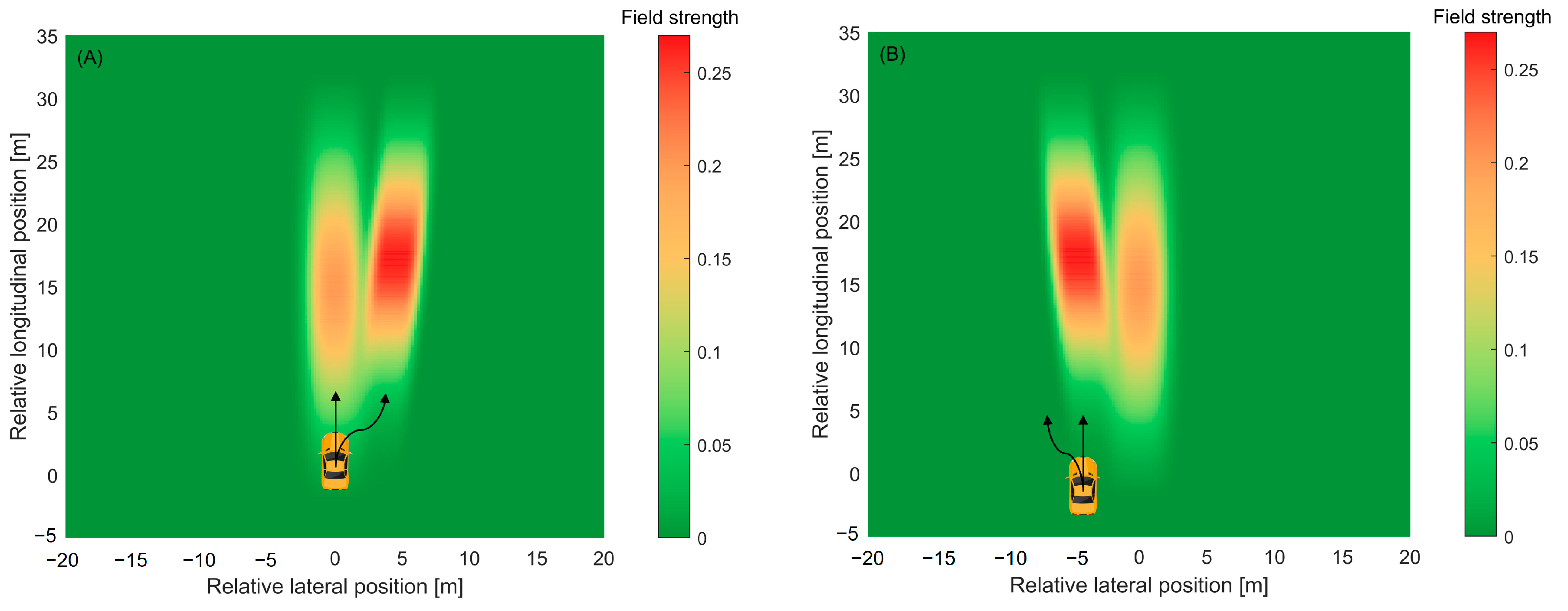
4.3. Driving Safety Field for Ramp Area

In Section 4.2, we introduced the method of quantifying vehicle behavior in ramp influence areas using Gaussian Mixture Models (GMMs). In this section, we apply the GMM to the safety field constructed in Section 4.1. First, we further segmented the road sections, with the segmentation results shown in Figure 6.

In this research, we solve the acceleration distribution for each area of ramp influencing area. The distribution of lateral and longitudinal acceleration often reflects the vehicle’s trends of movement. When the lateral acceleration is greater than 0, the vehicle tends to change lanes to the right. Similarly, when the acceleration is less than 0, the vehicle tends to change lanes to the left (as shown in Figure 7). The mean and variance of the Gaussian mixture distribution represent the meaning of corresponding traffic behavior, and the weight of each component represents the probability of this behavior occurring in the given area.

Based on the distribution of acceleration, the traffic behaviors under different road environments can be captured by different components of the GMM model.

$$f\left(a_{n,t}^x,a_{n,t}^y|R\right)=\sum _{i=1}^k{\alpha }_{i}N({\mathit{\mu }}_{\mathit{i}},{\mathsf{\Sigma }}_{\mathit{i}})$$

(21)

For example, Figure 8 provides a detailed realization of this safety field. In the ramping areas, the vehicles will always change their way to exit or enter the ramp. It can be reflected by the acceleration (especially lateral acceleration). The component of the GMM model represents the probability of each type of behavior. And the vehicles near the ramp will have a strong interaction with the vehicles in the adjacent lane. The intention of this lane changing can be captured with our safety field (the intention of turning right can be found in Figure 8A and the intention of turning left can be found in Figure 8B).

5. Results and Discussion

5.1. Calibration of Parameters in Driving Safety Field

This study focuses on ramp influence areas, so we examine segments U2, U3, U4, U7, U8, and U9. First, we determine the optimal number of the Gaussian distributions by calculating the likelihood function. The results show that the vehicle trajectory data on segments U2 and U7, which are located on the main lanes, consist of only one Gaussian distribution. The likelihood function curves for segments U3, U4, U8, and U9, with respect to the number of distributions, are shown in Figure 9. By observing the curves, we determine the optimal number of distributions as the points where the growth rate of the log-likelihood value significantly slows down, corresponding to 4, 2, 4, and 2 distributions, respectively.

After determining the optimal number of distributions, we solve the GMM model with the EM algorithm. The results of the GMM are shown in

Table 2. Results of Gaussian Mixture Model.

Segment	Number of Components	Weight	Mean Vector	Covariance Matrix
$U3$	1	$0.1444$	$[-\mathrm{0.0489,\; 0.2347}]$	$[\begin{array}{cc}0.6623& -0.1697\\ -0.1697& 2.5255\end{array}]$
	2	$0.2477$	$[0.0272, 0.1208]$	$[\begin{array}{cc}0.007& 0.0053\\ 0.0053& 0.2924\end{array}]$
	3	0.3043	$[-0.4021, 0.4082]$	$[\begin{array}{cc}0.368& -0.084\\ -0.084& 0.8233\end{array}]$
	4	0.3036	$[0.018, 0.1047]$	$[\begin{array}{cc}0.0696& -0.0168\\ -0.0168& 1.8166\end{array}]$
$U4$	1	0.8960	$[0.003, 0.1274]$	$[\begin{array}{cc}0.1047& -0.0379\\ -0.0379& 1.2101\end{array}]$
	2	0.1040	$[-1.4526, 1.3151]$	$[\begin{array}{cc}2.4333& 0.2845\\ 0.2845& 8.2473\end{array}]$
$U8$	1	0.1445	$[-\mathrm{0.0154,\; 0.0218}]$	$[\begin{array}{cc}0.0021& 0.0005\\ 0.0005& 0.0575\end{array}]$
	2	0.6069	$[-0.1217,-0.1773]$	$[\begin{array}{cc}0.2209& 0.392\\ 0.392& 1.7481\end{array}]$
	3	0.0737	$[1.0308, 2.6137]$	$[\begin{array}{cc}0.0574& 0.0479\\ 0.0479& 0.4402\end{array}]$
	4	0.1750	$[-0.1119,-0.1314]$	$[\begin{array}{cc}0.7185& 0.5531\\ 0.5531& 3.5895\end{array}]$
$U9$	1	0.8146	$[0.2236, 0.0171]$	$[\begin{array}{cc}0.2594& 0.1434\\ 0.1434& 0.6153\end{array}]$
	2	0.1854	$[-0.0949,-0.5599]$	$[\begin{array}{cc}1.8767& 0.1318\\ 0.1318& 7.9779\end{array}]$

.

According to the results of the Gaussian Mixture Model, we can describe the behaviors in each area as shown in Figure 10. For example, on the U3 segment, there is a 30.43% probability that a vehicle will travel with a lateral acceleration of 0.4021 m/s² to the left and a longitudinal acceleration of 0.4082 m/s² forward. The other three components indicate that the vehicle will keep its lane and go straight with about a 70% probability. After obtaining the acceleration distribution $\mathrm{f}\left({\mathrm{a}}_{\mathrm{n},\mathrm{t}}^{\mathrm{x}},{\mathrm{a}}_{\mathrm{n},\mathrm{t}}^{\mathrm{y}}\right)$, we set the $∆\mathrm{t}$ = 3 s because in most collision warning systems, the advanced warning time is about 3 s.

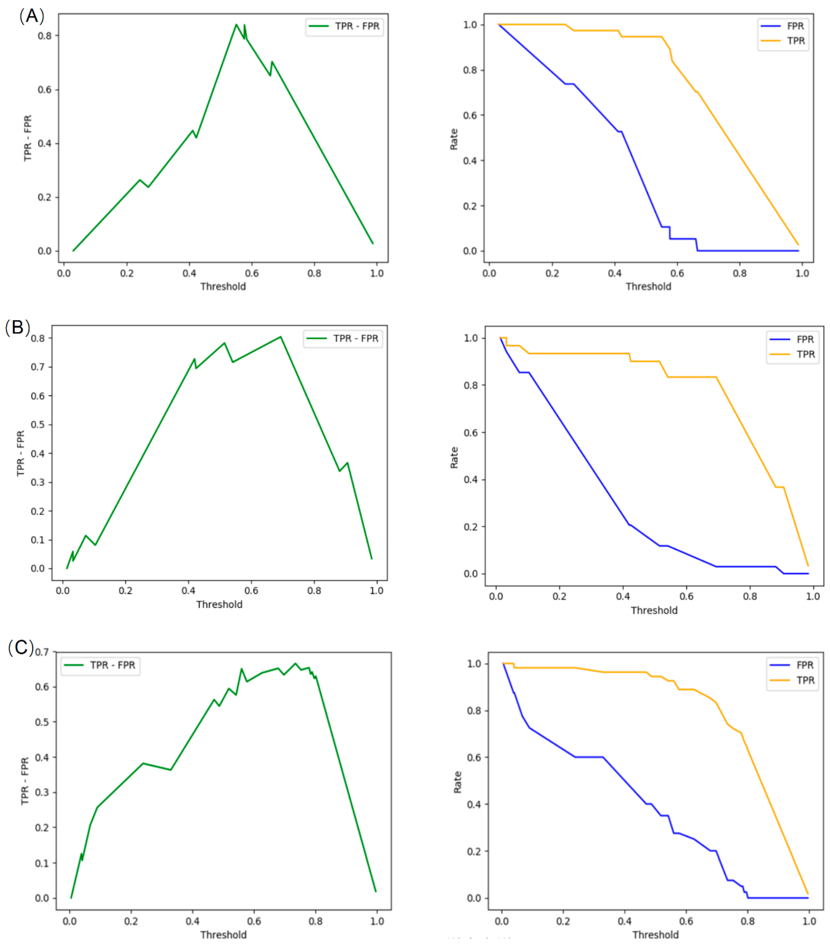
5.2. Finding the Critical-Event Threshold for the Driving Safety Field

In Section 5.1, we calibrated the relevant parameters. In this section, we will calibrate the best threshold of alarm (identifying dangerous events). As a safety assessment method, an important evaluation is to calibrate the threshold between safety and dangerous events. To enhance the effectiveness of safety assessment methods and driver acceptance when integrating these methods into ADASs, the threshold should closely align with drivers’ perception of risk.

The confusion matrix is often used to quantify the performance of classification algorithms. It displays the relationship between the actual categories and model-predicted categories. In this study, we use a confusion matrix to determine whether the perceived danger scene by the driver is consistent with the danger scene identified based on the driving safety field. The scene is divided into four categories, including TP, FN, FP, and TN. Among them, TP represents true positive, which is the number of samples that are actually positive and correctly predicted as positive (both the driver and the safety field determine that this scene is dangerous); FN stands for false negative, which refers to the number of samples that are actually positive but are incorrectly predicted as negative (the driver perceives danger but the safety field fails to recognize it); FP represents false positive, which refers to the number of samples that are actually negative but incorrectly predicted as positive (the driver considers it safe but the safety field judges it as dangerous); TN represents true negative, which refers to the number of samples that are actually negative and correctly predicted as negative (both the driver and the safety field consider it safe). A reasonable classification algorithm needs to maximize the true positive rate (TPR) and minimize the false positive rate (TPR) as much as possible. The TPR and FPR can be calculated as follows:

$$TPR={\displaystyle \frac{TP}{TP+FN}}$$

(22)

$$FPR={\displaystyle \frac{FP}{TN+FP}}$$

(23)

We extracted some vehicle trajectory fragments from the NGSIM dataset as typical driving scenarios, then we sequentially compared them with video files to ensure the correctness and typicality of the scenarios. Based on the research of Moon et al. [32], representative scenarios of safety (longitudinal deceleration > −2 m/s²) and danger (longitudinal deceleration < −4 m/s²) can be determined by the longitudinal deceleration of vehicles in the scenario. Firstly, we need to determine the optimal threshold for driving safety based on the driver’s reaction. We select this threshold by maximizing the (TPR-FPR).

The optimal threshold and curves of TPR and FPR for different road sections are shown in Figure 11. Overall, at each road section, a safety field strength of 0.6 is a good threshold for safety and risky event segmentation. We use this value as the threshold for identifying hazardous events. In addition, this result also indicates that our method is applicable to different road types, as they have similar thresholds.

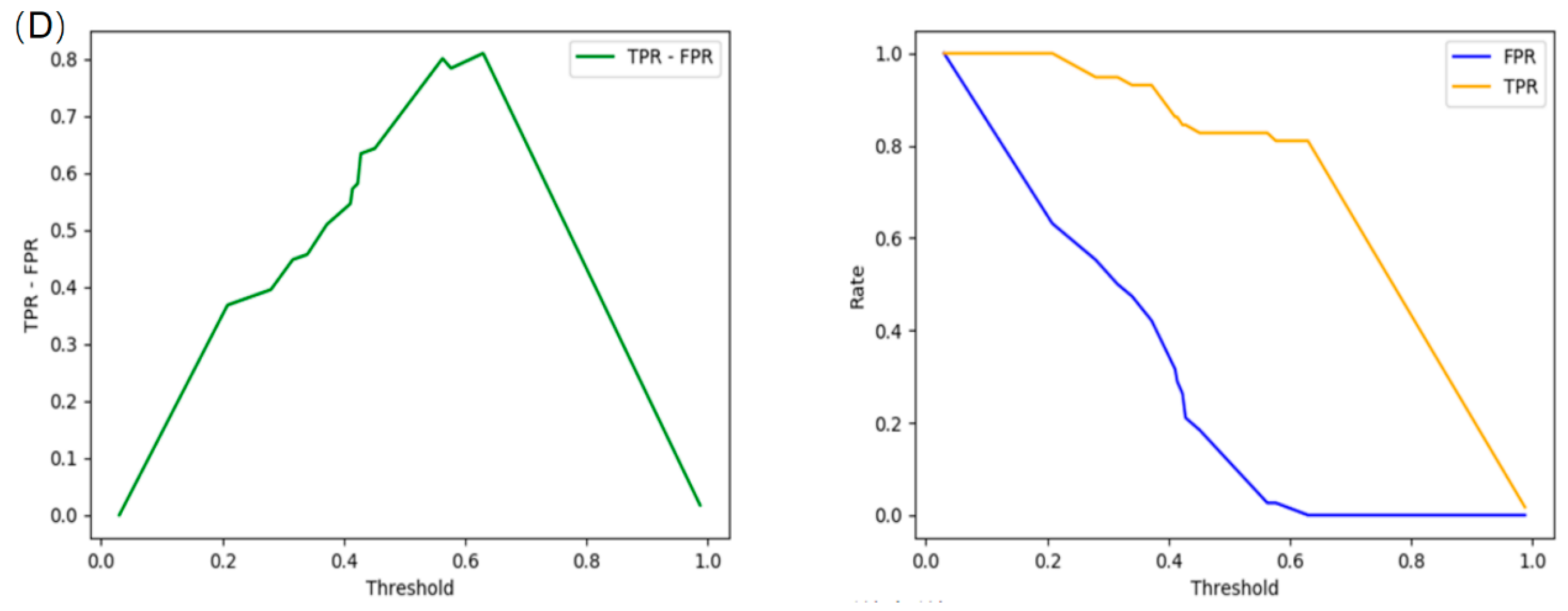
5.3. Comparing Driving Safety Field with Time to Collision

In this section, we will verify the effectiveness of the proposed method. Our verification will be carried out from the perception of the drivers. The dangerous situations identified by our proposed method need to be consistent with risky events identified by the driver. We will explain it by the confusion matrix and Receiver Operating Characteristic (ROC) curve. In addition, we will conduct simulations of hypothetical scenarios in ramp influence areas and compare the performance of Time to Collision (TTC) and driving safety field in identifying hazardous events.

Based on the TPR and FPR in Section 5.2, we will provide ROC (Receiver Operating Characteristic) curves for the safety hazard scenario classification. The ROC curve displays the performance of the model by plotting the relationship between the true class rate (TPR) and false positive class rate (FPR) at different thresholds. Generally, the larger the area below the ROC curve (ranging from 0 to 1, recorded as AUG), the better the classification performance. The ROC curves of TTC and our proposed driving safety field can be found in Figure 12A,B.

In Figure 12A, the ROC curve for Time to Collision (TTC) is displayed. The AUC value for TTC is approximately 0.57, indicating a relatively poor performance in distinguishing between safe and hazardous scenarios. The curve shows that TTC has limited effectiveness in accurately classifying safety hazards, as the area under the curve is close to 0.5, which is the performance of a random classifier. This is because TTC often overlooks adjacent lanes, making it difficult to handle hazardous events in ramp influencing aeras.

In Figure 12B, the ROC curve for the proposed driving safety field is shown. The AUC value for the driving safety field is approximately 0.71, indicating a much better performance in classifying safety hazards compared to TTC. The curve demonstrates a significantly higher true positive rate across various thresholds, showcasing the enhanced capability of the driving safety field in accurately identifying hazardous events. The substantial difference in AUC values between the two methods highlights the superior performance of the driving safety field over TTC in real-time safety assessments of ramp influencing areas.

To further explain the performance of our proposed driving safety field, we conducted simulations of hypothetical scenarios in ramp influence areas to compare the effectiveness of Time to Collision (TTC) and the driving safety field in identifying hazardous events. In this section, we use the inverse of Time to Collision (iTTC) to better clarify their performance. We set up two typical scenarios in areas before the exit ramp (corresponding to U8 in Section 4), including straightforward driving and lane-changing maneuvers. The scenario in Figure 13A serves as a baseline for straightforward driving behavior, while the scenario in Figure 13B highlights the challenges introduced by lane-changing maneuvers. By comparing these scenarios, we can evaluate the effectiveness of different safety assessment methods, such as TTC and the Dynamic Safety Field (DSF), in capturing the associated risks and providing real-time safety measures. Detailed trajectory information for these two scenarios can be found in Figure 13C,D.

In the scenario depicted in Figure 13A, the front (neighboring) vehicle starts at a lateral position of −3.5 m and a longitudinal position of 200 m, with a constant longitudinal speed of 10 m/s. The subject vehicle starts with the same lateral position and is 20 m behind the front vehicle, driving faster with a constant longitudinal speed of 12 m/s. As the subject vehicle approaches and eventually overtakes the front vehicle, the DSF and iTTC values both increase rapidly. Considering the threshold for iTTC is 0.3 s⁻¹, both DSF and iTTC effectively capture the dynamic risk in this scenario.

In the scenario depicted in Figure 13B, the front (neighboring) vehicle again starts at a lateral position of −3.5 m and a longitudinal position of 180 m, with a constant longitudinal speed of 12 m/s. In this scenario, the two vehicles are located in different lanes. The subject vehicle starts at a lateral position of 0 m, which is 20 m ahead of the front vehicle, with a constant longitudinal speed of 10 m/s. At time t = 5 s, the front vehicle initiates a lane-change maneuver to the adjacent lane, introducing lateral movement in addition to its longitudinal trajectory. During this lane-changing process, the longitudinal velocity remains unchanged, the transverse velocity is expressed by a sine function, and the lane-changing duration is 5 s. As the subject vehicle continues in its lane without slowing down, the risk of crash increases. In this scenario, DSF values increase significantly during the lane-change period, reflecting the heightened risk due to the merging action. Meanwhile, iTTC fails to capture this risk timely. This simulation indicates that the DSF is sensitive to lane-change behavior and provides a comprehensive risk assessment, whereas iTTC, which is based on relative longitudinal speed and position differences, may not fully capture the risk in complex scenarios involving lane changes.

Overall, the simulation results indicate that the Dynamic Safety Field (DSF) is more effective than iTTC in identifying hazardous events in complex traffic scenarios such as in ramp influence areas. The DSF’s ability to capture the risk associated with lateral movements and lane changes makes it a valuable tool for real-time safety assessment and the design of Advanced Driver Assistance Systems (ADASs). This enhanced performance highlights the potential of the DSF to provide more accurate and reliable safety measures, particularly in environments where traditional methods like TTC may fall short.

6. Conclusions

This study presents a novel approach to real-time safety assessments in ramp influence areas on highways by developing a driving safety field (DSF). Traditional safety assessment methods, such as Time to Collision (TTC), often fall short in capturing the complexities of traffic scenarios involving frequent merging and lane-changing maneuvers. The DSF, by incorporating the uncertainties of vehicle movements and integrating characteristics of driving behaviors, vehicles, and road environments, addresses these gaps effectively. Our research validated the DSF through simulations using the NGSIM dataset, focusing on scenarios typical of ramp influence areas. The results demonstrated that the DSF significantly outperforms TTC in identifying hazardous events, particularly in complex traffic environments. The DSF’s sensitivity to lateral movements and lane changes provides a more comprehensive and accurate real-time risk assessment, which is crucial for enhancing the effectiveness of Advanced Driver Assistance Systems (ADASs). According to the verification based on the NGSIM dataset, our proposed DSF outperforms other traditional measures such as TTC. This advantage is mainly reflected in the following aspects:

(1) In the ramp influence areas, the DSF method we proposed takes into account the road characteristics and the driver’s intention, so it is closer to the driver’s safety perception (see the ROC curve in Figure 12).

(2) The proposed method considers the potential collision events of adjacent lanes, so it can accurately and timely identify the dangerous events in the ramp influencing area, while current measures like TTC fail to identify these critical events timely.

The limitations of this study are as follows: Firstly, we only utilized the NGSIM dataset, indicating that the generalizability of our model requires further validation. Additionally, in practical applications, the parameters of the Gaussian Mixture Model (GMM) need to be re-calibrated according to specific road conditions, more datasets should be applied for further verifications and calibrations of the proposed model. Lastly, although our method significantly outperforms the TTC, the ROC curve’s AUC is still only 0.71. This may be due to the inclusion of scenarios where drivers decelerate without perceiving any real danger, suggesting that the selected scenarios may require further refinement. In future work, firstly, we will further develop our model and focus on more extensive factors including, but not limited to, traffic flow states and driving styles. On this basis, we plan to use driving simulation technology to further investigate the proposed DSF. Additionally, we will focus on designing a collision avoidance ADAS based on the DSF, which may contribute to safer and more reliable advanced driver assistance systems.

References

1. World Health Organization. Global Status Report on Road Safety 2018; World Health Organization: Geneva, Switzerland, 2019. [Google Scholar]
2. Corona, D.; De Schutter, B. Adaptive cruise control for a SMART car: A comparison benchmark for MPC-PWA control methods. IEEE Trans. Control Syst. Technol. 2008, 16, 365–372. [Google Scholar] [CrossRef]
3. Miaou, S.P.; Lum, H. Modeling vehicle accidents and highway geometric design relationships. Accid. Anal. Prev. 1993, 25, 689–709. [Google Scholar] [CrossRef] [PubMed]
4. Bauer, K.M.; Harwood, D.W. Statistical Models of Accidents on Interchange Ramps and Speed-Change Lanes; United States Federal Highway Administration: Washington, DC, USA, 1997.
5. Eller, E.; Frey, D. Psychological perspectives on perceived safety: Social factors of feeling safe. In Perceived Safety; Springer: Cham, Switzerland, 2019; pp. 43–60. [Google Scholar] [CrossRef]
6. Garnowski, M.; Manner, H. On factors related to car accidents on German Autobahn connectors. Accid. Anal. Prev. 2011, 43, 1864–1871. [Google Scholar] [CrossRef] [PubMed]
7. Xu, C.; Liu, P.; Wang, W. Evaluation of the predictability of real-time crash risk models. Accid. Anal. Prev. 2016, 94, 207–215. [Google Scholar] [CrossRef]
8. Zheng, L.; Sayed, T.; Mannering, F. Modeling traffic conflicts for use in road safety analysis: A review of analytic methods and future directions. Anal. Methods Accid. Res. 2021, 29, 100142. [Google Scholar] [CrossRef]
9. Xu, Y.; Ye, W.; Xie, Y.; Wang, C. A two-dimensional surrogate safety measure based on fuzzy logic model. Accid. Anal. Prev. 2024, 199, 107529. [Google Scholar] [CrossRef]
10. Xiong, X.; He, Y.; Gao, X.; Zhao, Y. A Multi-Level Risk Framework for Driving Safety Assessment Based on Vehicle Trajectory. Promet-Traffic Transp. 2022, 34, 959–973. [Google Scholar] [CrossRef]
11. Hu, J.J.; Li, F.; Han, B.; Yao, J. Analysis of the influence on expressway safety of ramps. Arch. Transp. 2017, 43, 43–51. [Google Scholar] [CrossRef]
12. Chu, H.; Zhuang, H.; Wang, W.; Na, X.; Guo, L.; Zhang, J.; Cao, B.; Chen, H. A review of driving style recognition methods from short-term and long-term perspectives. IEEE Trans. Intell. Veh. 2023, 8, 4599–4612. [Google Scholar] [CrossRef]
13. Wang, W.; Xi, J.; Zhao, D. Driving style analysis using primitive driving patterns with Bayesian nonparametric approaches. IEEE Trans. Intell. Transp. Syst. 2018, 20, 2986–2998. [Google Scholar] [CrossRef]
14. Johnson, D.A.; Trivedi, M.M. Driving style recognition using a smartphone as a sensor platform. In Proceedings of the 2011 14th International IEEE conference on intelligent transportation systems (ITSC), Washington, DC, USA, 5–7 October 2011; IEEE: New York, NY, USA; pp. 1609–1615. [Google Scholar]
15. Shao, Y.; Shi, X.; Zhang, Y.; Zhang, Y.; Xu, Y.; Chen, W.; Ye, Z. Adaptive forward collision warning system for hazmat truck drivers: Considering differential driving behavior and risk levels. Accid. Anal. Prev. 2023, 191, 107221. [Google Scholar] [CrossRef] [PubMed]
16. Zhu, J.; Tasic, I. Safety analysis of freeway on-ramp merging with the presence of autonomous vehicles. Accid. Anal. Prev. 2021, 152, 105966. [Google Scholar] [CrossRef] [PubMed]
17. Wang, J.; Yu, C.; Li, S.E.; Wang, L. A forward collision warning algorithm with adaptation to driver behaviors. IEEE Trans. Intell. Transp. Syst. 2015, 17, 1157–1167. [Google Scholar] [CrossRef]
18. Li, L.; Gan, J.; Qu, X.; Lu, W.; Mao, P.; Ran, B. A dynamic control method for cavs platoon based on the MPC framework and safety potential field model. KSCE J. Civ. Eng. 2021, 25, 1874–1886. [Google Scholar] [CrossRef]
19. Mullakkal-Babu, F.A.; Wang, M.; He, X.; van Arem, B.; Happee, R. Probabilistic field approach for motorway driving risk assessment. Transp. Res. Part C Emerg. Technol. 2020, 118, 102716. [Google Scholar] [CrossRef]
20. Kolekar, S.; De Winter, J.; Abbink, D. Human-like driving behaviour emerges from a risk-based driver model. Nat. Commun. 2020, 11, 1–13. [Google Scholar] [CrossRef]
21. Miaou, S.P. The relationship between truck accidents and geometric design of road sections: Poisson versus negative binomial regressions. Accid. Anal. Prev. 1994, 26, 471–482. [Google Scholar] [CrossRef]
22. El-Basyouny, K.; Sayed, T. Comparison of two negative binomial regression techniques in developing accident prediction models. Transp. Res. Rec. 2006, 1950, 9–16. [Google Scholar] [CrossRef]
23. Lord, D.; Miranda-Moreno, L.F. Effects of low sample mean values and small sample size on the estimation of the fixed dispersion parameter of Poisson-gamma models for modeling motor vehicle crashes: A Bayesian perspective. Saf. Sci. 2008, 46, 751–770. [Google Scholar] [CrossRef]
24. Guo, Y.; Liu, P.; Liang, Q.; Wang, W. Effects of parallelogram-shaped pavement markings on vehicle speed and safety of pedestrian crosswalks on urban roads in China. Accid. Anal. Prev. 2016, 95, 438–447. [Google Scholar] [CrossRef]
25. Alarifi, S.A.; Abdel-Aty, M.; Lee, J. A Bayesian multivariate hierarchical spatial joint model for predicting crash counts by crash type at intersections and segments along corridors. Accid. Anal. Prev. 2018, 119, 263–273. [Google Scholar] [CrossRef] [PubMed]
26. Bauer, K.M.; Harwood, D.W. Safety effects of horizontal curve and grade combinations on rural two-lane highways. Transp. Res. Rec. 2013, 2398, 37–49. [Google Scholar] [CrossRef]
27. Laureshyn, A.; Svensson, Å.; Hydén, C. Evaluation of traffic safety, based on micro-level behavioural data: Theoretical framework and first implementation. Accid. Anal. Prev. 2010, 42, 1637–1646. [Google Scholar] [CrossRef]
28. Thomas, I. Spatial data aggregation: Exploratory analysis of road accidents. Accid. Anal. Prev. 1996, 28, 251–264. [Google Scholar] [CrossRef] [PubMed]
29. Mountain, L.; Maher, M.; Fawaz, B. The influence of trend on estimates of accidents at junctions. Accid. Anal. Prev. 1998, 30, 641–649. [Google Scholar] [CrossRef] [PubMed]
30. Washington, S.; Karlaftis, M.G.; Mannering, F.; Anastasopoulos, P. Statistical and Econometric Methods for Transportation Data Analysis; Chapman and Hall/CRC: Boca Raton, FL, USA, 2020. [Google Scholar]
31. Islam, Z.; Abdel-Aty, M. Traffic conflict prediction using connected vehicle data. Anal. Methods Accid. Res. 2023, 39, 100275. [Google Scholar] [CrossRef]
32. Orsini, F.; Gecchele, G.; Rossi, R.; Gastaldi, M. A conflict-based approach for real-time road safety analysis: Comparative evaluation with crash-based models. Accid. Anal. Prev. 2021, 161, 106382. [Google Scholar] [CrossRef]
33. Formosa, N.; Quddus, M.; Ison, S.; Abdel-Aty, M.; Yuan, J. Predicting real-time traffic conflicts using deep learning. Accid. Anal. Prev. 2020, 136, 105429. [Google Scholar] [CrossRef]
34. Laureshyn, A.; De Ceunynck, T.; Karlsson, C.; Svensson, Å.; Daniels, S. In search of the severity dimension of traffic events: Extended Delta-V as a traffic conflict indicator. Accid. Anal. Prev. 2017, 98, 46–56. [Google Scholar] [CrossRef]
35. Moon, S.; Moon, I.; Yi, K. Design, tuning, and evaluation of a full-range adaptive cruise control system with collision avoidance. Control Eng. Pract. 2009, 17, 442–455. [Google Scholar] [CrossRef]
36. Minderhoud, M.M.; Bovy, P.H. Extended time-to-collision measures for road traffic safety assessment. Accid. Anal. Prev. 2001, 33, 89–97. [Google Scholar] [CrossRef] [PubMed]
37. Songchitruksa, P.; Tarko, A.P. Practical method for estimating frequency of right-angle collisions at traffic signals. Transp. Res. Rec. 2006, 1953, 89–97. [Google Scholar] [CrossRef]
38. Van Beinum, A.; Farah, H.; Wegman, F.; Hoogendoorn, S. Critical assessment of methodologies for operations and safety evaluations of freeway turbulence. Transp. Res. Rec. 2016, 2556, 39–48. [Google Scholar] [CrossRef]
39. Wang, C.; Xie, Y.; Huang, H.; Liu, P. A review of surrogate safety measures and their applications in connected and automated vehicles safety modeling. Accid. Anal. Prev. 2021, 157, 106157. [Google Scholar] [CrossRef] [PubMed]
40. Eggert, J. Predictive risk estimation for intelligent ADAS functions. In Proceedings of the 17th International IEEE Conference on Intelligent Transportation Systems (ITSC), Qingdao, China, 8–11 October 2014; IEEE: New York, NY, USA; pp. 711–718. [Google Scholar]
41. Mullakkal-Babu, F.A.; Wang, M.; Farah, H.; van Arem, B.; Happee, R. Comparative assessment of safety indicators for vehicle trajectories on highways. Transp. Res. Rec. 2017, 2659, 127–136. [Google Scholar] [CrossRef]
42. Hwang, Y.K.; Ahuja, N. A potential field approach to path planning. IEEE Trans. Robot. Autom. 1992, 8, 23–32. [Google Scholar] [CrossRef]
43. Ni, D. A unified perspective on traffic flow theory, Part I: The field theory. In ICCTP 2011: Towards Sustainable Transportation Systems; ASCE: Reston, VA, USA, 2011; pp. 4227–4243. [Google Scholar]
44. Arun, A.; Haque, M.M.; Washington, S.; Mannering, F. A physics-informed road user safety field theory for traffic safety assessments applying artificial intelligence-based video analytics. Anal. Methods Accid. Res. 2023, 37, 100252. [Google Scholar] [CrossRef]
45. Wang, J.; Wu, J.; Zheng, X.; Ni, D.; Li, K. Driving safety field theory modeling and its application in pre-collision warning system. Transp. Res. Part C Emerg. Technol. 2016, 72, 306–324. [Google Scholar] [CrossRef]
46. Haule, H.J.; Ali, M.S.; Alluri, P.; Sando, T. Evaluating the effect of ramp metering on freeway safety using real-time traffic data. Accid. Anal. Prev. 2021, 157, 106181. [Google Scholar] [CrossRef]
47. Wahab, L.; Jiang, H. Severity prediction of motorcycle crashes with machine learning methods. Int. J. Crashworthiness 2019, 25, 485–492. [Google Scholar] [CrossRef]
48. Zhang, H.; Liang, J.; Jiang, H.; Cai, Y.; Xu, X. Stability research of distributed drive electric vehicle by adaptive direct yaw moment control. IEEE Access 2019, 7, 106225–106237. [Google Scholar] [CrossRef]
49. Cong, S.; Wang, W.; Liang, J.; Chen, L.; Cai, Y. An automatic vehicle avoidance control model for dangerous lane-changing behavior. IEEE Trans. Intell. Transp. Syst. 2021, 23, 8477–8487. [Google Scholar] [CrossRef]
50. Balke, K.; Chaudhary, N.; Songchitruksa, P.; Pesti, G. Development of Criteria and Guidelines for Installing, Operating, and Removing TxDOT Ramp Control Signals (No. FHWA/TX-09/0-5294-1); Texas Transportation Institute: College Station, TX, USA, 2009. [Google Scholar]
51. Zhao, J.; Guo, Y.; Liu, P. Safety impacts of geometric design on freeway segments with closely spaced entrance and exit ramps. Accid. Anal. Prev. 2021, 163, 106461. [Google Scholar] [CrossRef]
52. van Beinum, A.; Farah, H.; Wegman, F.; Hoogendoorn, S. Driving behaviour at motorway ramps and weaving segments based on empirical trajectory data. Transp. Res. Part C Emerg. Technol. 2018, 92, 426–441. [Google Scholar] [CrossRef]
53. Kwak, H.C.; Kho, S. Predicting crash risk and identifying crash precursors on Korean expressways using loop detector data. Accid. Anal. Prev. 2016, 88, 9–19. [Google Scholar] [CrossRef]
54. Kusuma, A.; Liu, R.; Choudhury, C.; Montgomery, F. Lane-changing characteristics at weaving section. In Proceedings of the Transportation Research Board 94th Annual Meeting, Washington, DC, USA, 11–15 January 2015; Volume 94, pp. 49–55. [Google Scholar]
55. Colyar, J.; Halkias, J. US Highway101 Dataset; FHWA-HRT-07-030; Federal Highway Administration (FHWA): Washington, DC, USA, 2007.
56. Reynolds, D.A. Gaussian mixture models. Encycl. Biom. 2009, 741, 659–663. [Google Scholar]
Figure 1. Diagram of US-101 segment.
Systems 12 00370 g001
Figure 2. Calculation of velocity and acceleration by differentiation.
Systems 12 00370 g002
Figure 3. Speed distribution in the ramp.
Systems 12 00370 g003
Figure 4. Calculation of collision probability.
Systems 12 00370 g004
Figure 5. Safety field under different conditions: (A) t = 3 s, V n , t x = 0 m/s, V n , t y = 20 m/s, W s = W n = 1.8 m, L s = L n = 3.5 m, and ( a n , t x , a n , t y ) ~ N ( 0,0 , 0.2,0.5,0 ) ; (B) t = 3 s, V n , t x = 0 m/s, V n , t y = 25 m/s, W s = W n = 1.8 m, L s = L n = 3.5 m, and ( a n , t x , a n , t y ) ~ N ( 0,0 , 0.2,0.5,0 ) ; (C) t = 3 s, V n , t x = 0 m/s, V n , t y = 25 m/s, W s = 1.8 m, L s = 3.5 m, W n = 3 m, L n = 6 m, and ( a n , t x , a n , t y ) ~ N ( 0,0 , 0.2,0.5,0 ) ; and (D) t = 3 s, V n , t x = −0.5 m/s, V n , t y = 20 m/s, W s = W n = 1.8 m, L s = L n = 3.5 m, and ( a n , t x , a n , t y ) ~ N ( 0,0 , 0.2,0.5,0 ) .
Systems 12 00370 g005
Figure 6. Diagram of road sections segmentation.
Systems 12 00370 g006
Figure 7. Acceleration distribution under different lane-changing behaviors: (A) changing to the left lane and (B) changing to the right lane.
Systems 12 00370 g007
Figure 8. Driving safety field for ramp influencing area: (A) t = 3 s, V n , t x = V s , t x = 0 m/s, V n , t y = 20 m/s, V s , t y = 15 m/s, W s = W n = 1.8 m, L s = L n = 3.5 m, N 1 = N ( 0,0 , 0.2,1.5,0 ) , α 1 = 0.5, N2 = N(1,0.5,0.2,1.5,0.8), and α 2 = 0.5 and (B) t = 3 s, V n , t x = V s , t x = 0 m/s, V n , t y = 20 m/s, V s , t y = 15 m/s, W s = W n = 1.8 m, L s = L n = 3.5 m, N 1 = N ( 0,0 , 0.2,1.5,0 ) , α 1 = 0.5, N2 = N(−1,0.5,0.2,1.5,−0.8), and α 2 = 0.5.
Systems 12 00370 g008
Figure 9. The likelihood function curves of GMM model: (A) segment of U3; (B) segment of U4; (C) segment of U8; and (D) segment of U9.
Systems 12 00370 g009
Figure 10. Driving behaviors in each ramp influencing area.
Systems 12 00370 g010
Figure 11. True positive rate (TPR) and false positive rate (FPR) under different thresholds: (A) segment of U3; (B) segment of U4; (C) segment of U8; and (D) segment of U9.
Systems 12 00370 g011aSystems 12 00370 g011b
Figure 12. The ROC curves for TTC (A) and driving safety field (B).
Systems 12 00370 g012aSystems 12 00370 g012b
Figure 13. Simulation of the DSF and TTC’s performance in identifying risky events: (A) scenario of going straightforward; (B) scenario of lane-changing behavior; (C) the performance of DSF and TTC in the going straightforward scenario; and (D) the performance of DSF and TTC in the lane-changing scenario.
Systems 12 00370 g013aSystems 12 00370 g013b