Abstract
The purpose of this paper is to examine the optimization of the HIV drug supply chain, with a dual focus on minimizing freight costs and delivery times. With the help of a dataset containing 10,325 instances of supply chain transactions, key variables, including “Country”, “Vendor INCO Term”, and “Shipment Mode”, were examined in order to develop a predictive model using Artificial Neural Networks (ANN) employing a Multi-Layer Perceptron (MLP) architecture. A set of ANN models were trained to forecast “freight cost” and “delivery time” based on four principal design variables: “Line Item Quantity”, “Pack Price”, “Unit of Measure (Per Pack)”, and “Weight (Kilograms)”. According to performance metrics analysis, these models demonstrated predictive accuracy following training. An optimization algorithm, configured with an “active-set” algorithm, was then used to minimize the combined objective function of freight cost and delivery time. Both freight costs and delivery times were significantly reduced as a result of the optimization. This study illustrates the potent application of machine learning and optimization algorithms to the enhancement of supply chain efficiency. This study provides a blueprint for cost reduction and improved service delivery in critical medication supply chains based on the methodology and outcomes.
1. Introduction
The global fight against HIV/AIDS requires not only medical innovation but also a robust and efficient supply chain to ensure that life-saving antiretroviral (ARV) drugs reach those in need. The importance of optimizing the HIV drug supply chain cannot be overstated since it directly impacts care and treatment programs throughout the world. UNAIDS’ 90-90-90 targets aim to have 90% of HIV-infected individuals aware of their status, 90% of those diagnosed receiving antiretroviral therapy (ART), and 90% of those treated, achieving viral suppression by 2020 [1]. The distribution of HIV/AIDS commodities, including ARVs, requires both effective care delivery programs and an efficient supply chain. It has been a challenging journey to reach these goals. According to Alemnji et al. [2] HIV viral load and early infant diagnosis progress has been slowed in some countries due to gaps in access to HIV diagnostic tests. The Supply Chain Management System (SCMS) project delivered over USD 1.9 billion in HIV/AIDS commodities to support treatment, highlighting the importance of supply chain management in the fight against HIV/AIDS, according to Larson et al. [3]. Despite these efforts, there are still gaps in diagnostic access and treatment for many countries and subpopulations, which pose a threat to the achievement of UNAIDS’ targets. Alemnji et al. [2] found that only 52% of HIV-exposed infants were tested within 8 weeks of birth in 23 surveyed countries in 2018, with many not receiving ART on time. The lack of sufficient access to viral load tests among priority populations in low- and middle-income countries is also highlighted by the fact that less than half of patients on antiretroviral therapy receive regular viral load tests. The challenges extend to the procurement and distribution of ARVs, where production and shipping delays can result in stockouts, which can lead to ART interruption for patients Despite its efforts, the SCMS project was unable to maintain a reliable, cost-effective, and secure supply chain, mainly due to the high cost of commodities [3,4]. In addition, the HIV drug optimization agenda faces additional obstacles, as most clinical trials of new ARV agents are conducted among adults before including adolescents, children, and infants, which delays the availability of optimal new ARV regimens for these vulnerable groups [5]. As a result of these challenges, a multifaceted approach is required, which involves improving not only procurement and distribution systems but also ensuring that timely diagnosis and treatment are initiated. In the global effort to end the HIV/AIDS pandemic, a well-functioning HIV drug supply chain is of vital importance beyond the immediate needs of patients. It has been noted by Cao [6] and Schouten et al. [7] that an efficient supply chain is crucial to avoid stockouts and to ensure that the influx of resources is effectively allocated, particularly in resource-poor settings. Hence, optimizing the HIV drug supply chain is not only a logistical necessity but also an essential part of the global health response to HIV/AIDS.
Especially in low- and middle-income countries, supply chain management plays a critical role in the fight against HIV/AIDS. Stulens et al. [8] provide an in-depth analysis of the challenges and opportunities within HIV supply chains, emphasizing the need to have efficient and effective operations in order to increase the availability and accessibility of HIV services and supplies. In their research, they emphasize the importance of addressing these supply chain challenges through innovative operations research and operations management (OR/OM) solutions, highlighting an important area for future research and development. Furthermore, Jónasson et al. [9] demonstrated that optimization and simulation models can be used to improve early infant diagnosis (EID) supply chains in Sub-Saharan Africa. They have demonstrated that reassigning clinics to laboratories and consolidating diagnostic capacity can result in substantial reductions in sample turnaround times and a greater number of infected infants receiving treatment by applying their models to Mozambique’s EID program. There is a clear link between logistical optimizations and improved patient outcomes. The importance of continuous improvement in supply chain management practices is highlighted by these findings. Furthermore, Pastakia et al. [10] extend this discussion to the management of non-communicable diseases (NCDs), drawing lessons from HIV supply chain initiatives. Research suggests that strategies developed for HIV supply chains, such as addressing resource mobilization and utilization challenges, can be adapted to improve NCD supply chain systems in low- and middle-income countries. The cross-disease learning emphasizes the interconnectedness of healthcare supply chains and the potential for broader application of effective HIV supply chain management techniques. The first step was to develop robust ANN models that can accurately predict “freight cost” and “delivery time” within the HIV drug supply chain. This model contributes to the literature by providing a nuanced understanding of the factors affecting supply chain efficiency. Secondly, using the Fmincon algorithm in MATLAB (R2024a version), we applied advanced nonlinear optimization techniques to minimize these critical metrics. A novel and practical approach to decision-making in supply chain management is offered by our research, which bridges the gap between machine learning predictive capabilities and optimization methods. In addition, this study sets a precedent for the use of data-driven techniques in healthcare logistics, which may serve as a guide for future efforts in this field.
2. A Literature Review
Ahmad et al. [11] developed a multi-objective model to optimize the phasocio-economic performance of pharmaceutical supply chains with socio-economic and environmental objectives, ensuring optimal product allocation among different echelons under uncertainty. Using the Techniques for Order Preference by Similarity to Ideal Solution (TOPSIS) and other criteria, they demonstrated the importance of sustainable objectives in decision-making, which reduces economic costs, improves customer service, and reduces environmental impact. This approach aligns closely with the goals of enhancing efficiency in healthcare supply chains by considering socio-economic performance and sustainability in the optimization process. It is a reflection of problems prevalent in many low-to-medium-income countries that Olutuase et al. [12] conducted a scoping review on the challenges faced by medicines and vaccine supply chains in Nigeria. Factors such as procurement difficulties, inadequate storage, and distribution challenges contribute to stockouts and hinder access to essential medicines. In healthcare supply chains, logistical inefficiencies and infrastructure deficiencies must be addressed through optimization strategies. Lugada et al. [13] explored the structure, performance, and challenges of Uganda’s health supply chain system, emphasizing the need for improved policy implementation and infrastructure. Taking into account the inefficiencies in the health supply chain, optimization models that can enhance planning, coordination, and management across all levels of the health system are urgently needed.
Torrado and Barbosa [14] investigated the optimization and sustainability of blood supply chain networks under uncertainty from strategic–tactical and operational–tactical perspectives. Their literature review emphasizes the scarcity of blood products and the need for sustainable optimization to prevent shortages, wastage, and health risks. The insights gained from this study align with the challenges of optimizing the HIV drug supply chain, suggesting that environmental, economic, and social sustainability dimensions need to be considered. Saatchi et al. [15] proposed a bi-objective meta-heuristic algorithm to optimize relief logistics in humanitarian supply chains. For the distribution of commodities and transportation of injured individuals post-disaster, their model integrates a multi-echelon, forward and backward relief network. Compared to traditional algorithms, the hybrid non-dominated sorting genetic algorithm (NSGA-II) with simulated annealing (SA) and variable neighborhood search (VNS) demonstrated superior performance, emphasizing the importance of advanced optimization techniques in critical supply chain management. Tat et al. [16] study pharmaceutical supply chain coordination with a focus on minimizing leftover or end-of-life (EOL) medication waste. The mathematical model introduces a buyback and shortage risk-sharing contract (B&SRS) to reduce disposal costs and enhance channel profitability. In order to achieve supply chain coordination and sustainability, innovative contractual arrangements are necessary. Next-generation sequencing (NGS) provides sensitivity and cost-effectiveness advantages over traditional methods in HIV drug resistance testing, according to Ávila-Ríos et al. [17]. In spite of its potential, they noted significant challenges related to standardization, quality assurance, and implementation, particularly in resource-poor areas. In order to enhance diagnostic capabilities, technological advancements and infrastructure improvements are needed in healthcare supply chains. Siddiqui et al. [18] proposed a hybrid demand-forecasting model specifically designed for the pharmaceutical sector, integrating the Autoregressive Integrated Moving Average and Holt–Winters model (ARHOW). This model highlights the role of advanced forecasting in aligning production and distribution with market demand, thereby improving supply chain efficiency. Sindhwani et al. [19] analyzed the ability of a hub-and-spoke distribution network to mitigate ripple effects in the Indian pharmaceutical supply chain during the COVID-19 pandemic. Through a multi-layer approach involving Bayesian networks, mathematical optimization, and discrete event simulation, they provided strategies to enhance supply chain resilience and flexibility, which are critical for maintaining service levels during disruptions.
Singh et al. [20] utilized a simulation model to study the impact of COVID-19 on logistics and food supply chain disruptions, emphasizing the necessity of supply chain resilience. Their work underscores the challenges posed by the pandemic on the balance between supply and demand and proposes strategies to develop more robust and adaptable supply chains. Stulens [8] reviewed the challenges and opportunities of HIV supply chains in low- and middle-income countries, noting the lack of research in operations research/operations management (OR/OM) concerning HIV supply chains. Their findings stress the need for advanced modeling and optimization techniques to enhance efficiency and effectiveness in these contexts.
Jónasson et al. [9] presented a two-part modeling framework to optimize early infant diagnosis (EID) supply chains in Sub-Saharan Africa. Applied to Mozambique’s EID program, their optimization and simulation models demonstrated reductions in turnaround times and increased treatment rates for infected infants, highlighting the significant impact of logistical optimization on patient outcomes. Pastakia et al. [10] proposed that lessons from HIV supply chain initiatives could inform the management of noncommunicable disease (NCD) supply chains. They argued that advancements in HIV supply chain systems, particularly in resource mobilization and utilization, could be adapted to NCD supply chains with minimal additional investment. Jamieson and Kellerman [21] critically assessed the supply chain challenges of the UNAIDS “90-90-90” strategy, focusing on scaling up HIV diagnostics, antiretroviral therapy (ART) distribution, and viral load testing to meet global targets. Their study underscores the necessity of strong and resilient supply chains to support the global HIV response. Xiong et al. [22] demonstrated that optimizing clinical and logistical processes using operations research methodologies could enhance outcomes in HIV treatment scale-up. Key areas identified include forecasting, facility location and sizing, and staffing levels. Enyinda et al. [23] examined the New Partnership for HIV/AIDS Supply Chain Management (NPHASCM) initiative, emphasizing the challenges of healthcare supply chain management in Sub-Saharan Africa and the potential for partnerships to improve the timely delivery of life-saving HIV/AIDS commodities. This summary captures key studies on healthcare supply chain optimization, detailing the methodologies employed and the outcomes achieved across various disease areas. Rahimi et al. [24] developed a hybrid feature scoring approach, stressing the necessity of a staging system that incorporates diverse neurocognitive functions to improve understanding of PD. Ogunsoto et al. [25] introduced a digital twin framework for supply chain recovery, leveraging LSTM models for flood prediction and neural networks for post-disruption recovery, enabling informed strategies for resilience. Strika et al. [26] reviewed the role of AI and large language models in mitigating healthcare gaps in medical deserts, highlighting applications in telehealth, diagnostic assistance, and medical education while emphasizing the need for ongoing research to maximize their potential.
Artificial intelligence (AI) has played a crucial role in optimizing the COVID-19 pandemic therapeutics supply chain, particularly in at-risk communities, by enhancing efficiency and reducing delays in distribution [27]. Furthermore, machine learning techniques have significantly improved supply chain traceability and transparency, enabling better decision-making and operational efficiency in various industries [28,29]. Table 1 provides an overview of key studies on healthcare supply chain optimization, summarizing the methodologies, objectives, and key findings from various research efforts aimed at improving efficiency, cost-effectiveness, and service quality within the healthcare sector.

Table 1.
Overview of Key Studies on Healthcare Supply Chain Optimization.
From pharmaceuticals to blood supply to HIV treatment and humanitarian aid logistics, this overview provides insight into diverse approaches and results achieved in improving the efficiency, accessibility, and sustainability of healthcare supply chains.
3. Methods and Materials
3.1. Dataset Overview
The dataset used in this study was derived from the collaborative reporting systems of the Global Fund and PEPFAR. These organizations are the primary procurers of HIV health products and share a database known as the Price, Quality, and Reporting (PQR) database. By integrating PQR data, we can gain a holistic view of global health expenditures on HIV-related commodities, enabling more informed decisions. The value of this dataset lies in the detailed description of price variations, observable trends, and the distribution of product volumes across countries. Despite the fact that the dataset provides a wealth of information for analyzing market dynamics, its application is not without limitations. The data may not provide definitive insights into the costs associated with moving specific items or products to particular countries or the lead time involved when used in isolation. Performing such an assessment requires a nuanced understanding of the dataset in conjunction with other logistical and geopolitical factors. Despite these considerations, the US government believes that the dataset is an essential tool for enabling stakeholders to make better-informed decisions. Its nature allows for a more nuanced understanding of the HIV drug supply chain, which is essential for optimizing operations and improving global healthcare delivery.
3.2. ANN Method
Artificial Neural Networks (ANN) serve as the basis for modeling complex relationships within the HIV drugs supply chain dataset. In this study, we employ a Multi-Layer Perceptron (MLP) architecture, a type of artificial neural network (ANN) known for its ability to approximate continuous functions. An MLP model consists of an input layer, multiple hidden layers, and an output layer. The neurons in each layer apply a weighted sum of inputs followed by a nonlinear activation function. In general, the neuron’s output can be expressed as follows:
where xi represents the input values; wi is the associated weights; b is the bias, and f is the activation function. To minimize the difference between predicted outputs and actual targets, weights (wi) and biases (b) are adjusted during the training process. Backpropagation is typically used to achieve this optimization, which involves calculating the gradient of the loss function with respect to each weight and iteratively updating the weights in the direction that minimizes the loss. In this study, two ANN models were developed: one to predict freight costs and the other to predict delivery times. Models were trained using a subset of the dataset, and their performance was validated using a separate dataset. In order to enable precise cost and time estimates, the models were refined to reflect the underlying dynamics of the supply chain.
3.3. Nonlinear Optimization (Fmin Algorithm)
The optimization component of our study utilized MATLAB’s Fmincon function, an algorithm designed for solving nonlinear optimization problems subject to constraints. The objective of the optimization was to identify the set of design variables that minimized the objective function, which, in our case, is the sum of the standardized “freight cost” and “delivery time” variables:
The design variable (x) must be positive and exceed 10% of the dataset’s average value:
An active-set algorithm developed by Fmincon was used, which was designed to deal with both linear and nonlinear constraints. The objective function is minimized by iteratively adjusting the variables in order to satisfy the constraints. The algorithm’s settings, including “ScaleProblem”, “ConstraintTolerance”, and “DiffMinChange”, were meticulously configured to enhance the precision and efficiency of the optimization process. By integrating ANN predictions into the optimization framework, we were able to leverage the predictive power of machine learning with the rigor of mathematical optimization to minimize costs and delivery times.
4. Results and Discussion
A paper detailing the optimization of the HIV drug supply chain focuses on minimizing critical factors such as “Delivered to Client Date” and “Freight Cost (USD)”. The dataset incorporates a range of variables across 10,325 cases, encapsulating various elements of the supply chain from country management to shipment specifics and product details.
During the optimization process, a Response Surface Methodology (RSM) approach was used, which is a collection of statistical and mathematical techniques used to model and analyze problems where a response of interest is influenced by a number of variables [30]. In the algorithm, the pseudocodes are as follows: Algorithms 1–4.
| Algorithm 1: Pseudocode for ANN model creation |
| Step 1: Preprocess the dataset. |
| Load (dataset) |
| Standardize the features (LineItemQuantity, PackPrice, UnitofMeasure, Weight) |
| Step 2: Create the ANN models for Freight Cost and Delivery Time |
| Initialize the ANN for Freight Cost with input, hidden layers, and output |
| Initialize the ANN for Delivery Time with input, hidden layers, and output |
| Set training parameters (e.g., learning rate, epochs) |
| Step 3: Train the ANN models |
| For each epoch in the number of epochs: |
| Forward propagate the inputs through the network |
| Calculate the error between the predicted and actual values |
| Backpropagate the error to update the weights |
| Update the weights and biases according to the learning rate |
| Step 4: Evaluate the models |
| Test the trained models on the testing set |
| Calculate the performance metrics (e.g., R-squared value) |
| Step 5: Define the optimization problem |
| Define the objective function to minimize f1 + f2 |
| Set the constraints for design variables to be positive and above 10% of their average |
| Algorithm 2: Pseudo MATLAB code for Fmin optimization |
| function optimizeSupplyChain |
| Define the average values for the constraints |
| avgLineItemQuantity = calculateAverage(LineItemQuantity) |
| avgPackPrice = calculateAverage(PackPrice) |
| avgUnitofMeasure = calculateAverage(UnitofMeasure) |
| avgWeight = calculateAverage(Weight) |
| Define the lower bounds based on the constraints |
| lb = [0.1 * avgLineItemQuantity, 0.1 * avgPackPrice, 0.1 * avgUnitofMeasure, 0.1 * avgWeight] |
| Define the initial guess for the design variables |
| initialGuess = [initialLineItemQuantity, initialPackPrice, initialUnitofMeasure, initialWeight] |
| Define the optimization options |
| options = optimoptions(@fmincon,‘Algorithm’,‘active-set’,... |
| ‘ScaleProblem’,‘obj-and-constr’,... |
| ‘ConstraintTolerance’, 1 × 10⁻⁷,... |
| ‘DiffMinChange’, 1 × 10⁻⁶) |
| Perform the optimization |
| [optimalValues, optimalObjective] = fmincon(@objectiveFunction, initialGuess, [], [], [], [], lb, [], @nonlinearConstraints, options) |
| De-standardize the optimal values |
| destandardizeOptimalValues(optimalValues) |
| Output the optimized non-normalized values and objective function results |
| disp(‘Optimized LineItemQuantity: ’ + string(optimalValues(1))) |
| disp(‘Optimized PackPrice: ’ + string(optimalValues(2))) |
| disp(‘Optimized UnitofMeasure: ’ + string(optimalValues(3))) |
| disp(‘Optimized Weight: ’ + string(optimalValues(4))) |
| disp(‘Optimized Freight Cost: ’ + string(optimalObjective(1))) |
| disp(‘Optimized Delivery Time: ’ + string(optimalObjective(2))) |
| end |
| Algorithm 3: Pseudocode Define the objective function |
| function obj = objectiveFunction(designVariables) |
| Predict the standardized Freight Cost and Delivery Time using ANN models |
| f1 = predictFreightCostANN(designVariables) |
| f2 = predictDeliveryTimeANN(designVariables) |
| Objective is to minimize the sum of the two predictions |
| obj = f1 + f2 |
| end |
| Algorithm 4: Define the nonlinear constraints function |
| function [c, ceq] = nonlinearConstraints(designVariables) |
| No nonlinear inequality constraints |
| c = [] |
| The nonlinear equality constraints (ceq) are defined as the difference between the variables and their bounds |
| ceq = designVariables − lb |
| end |
| Call the optimization function |
| optimizeSupplyChain |
4.1. Response Surface Methodology Using MLP
The primary step in the optimization process was the development of predictive models utilizing an Artificial Neural Network (ANN) with a Multi-Layer Perceptron (MLP) architecture. Two distinct models were constructed:
- A model for predicting “Freight Cost (USD)” as a function of “Line Item Quantity”, “Pack Price”, “Unit of Measure (Per Pack)”, and “Weight (Kilograms)”;
- A model for predicting “delivery time” as a function of the same variables.
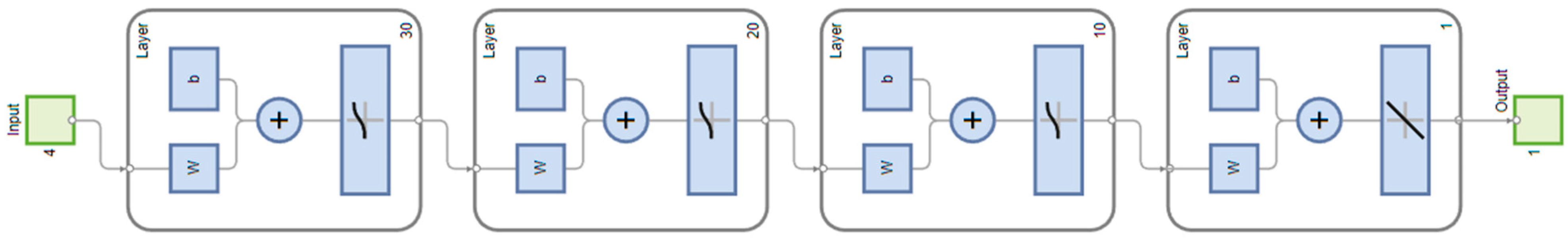
An MLP network was designed to accommodate the four selected design variables, followed by three hidden layers and an output layer (see Figure 1). The first hidden layer contained 30 neurons, the second—20 neurons, and the third—10 neurons, each utilizing a nonlinear activation function to capture the complex relationships between inputs and outputs There is a single neuron for each model in the output layer, which corresponds to the “freight cost” and “delivery time”, respectively. A promising foundation has been established in the initial phase of the optimization process, which involves training and validating the model. In order to optimize the HIV drug supply chain, it is imperative to be able to predict “freight cost” and “delivery time” effectively. Following this section, we will examine the application of these models within the RSM framework to identify optimal conditions that minimize the objectives of the problem, thus improving supply chain efficiency and reliability.
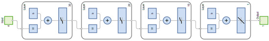
Figure 1.
Three hidden layers with 30, 20, and 10 nodes, respectively, and an output layer with 1 node.
It is crucial to understand the training progress of these models in order to determine their predictive capabilities and potential for optimization In training the “freight cost” model, the initial performance measure was 0.233, improving to a final value of 0.000481, near the target performance of 1 × 10⁻⁵. During training, the gradient, which is a measure of the error slope, started at 2.6 and decreased to 0.000151, which is satisfactory for understanding convergence. It took approximately 4 min and 13 s for the model to reach these results in over 30,000 epochs, indicating thorough training.
Comparatively, the “delivery time” model demonstrated an initial performance of 0.0659, which improved to 0.0019 after training. Although the final performance was not as close to the target as the “freight cost” model, the reduction in error suggests that the model can still provide valuable predictions for the optimization process. This model took slightly less time to train, taking 3 min and 54 s to complete the same number of epochs. As seen in the accompanying figures, these results illustrate the architecture of the MLP networks as well as the progression of the training process. As a graphical representation, the figures reinforce the quantitative results presented in the tables. It is evident from the results that the ANN MLP models have learned the underlying patterns in the dataset with a high degree of accuracy, as evidenced by the low post-training performance values. It is important to note that the success of these models depends upon the quality and preprocessing of the dataset, as well as the careful design of the neural network architecture. The training process is summarized in Table 2, which presents the initial, stopped, and target values for key parameters such as performance, gradient, and validation checks
Table 2.
Summary of the training process.
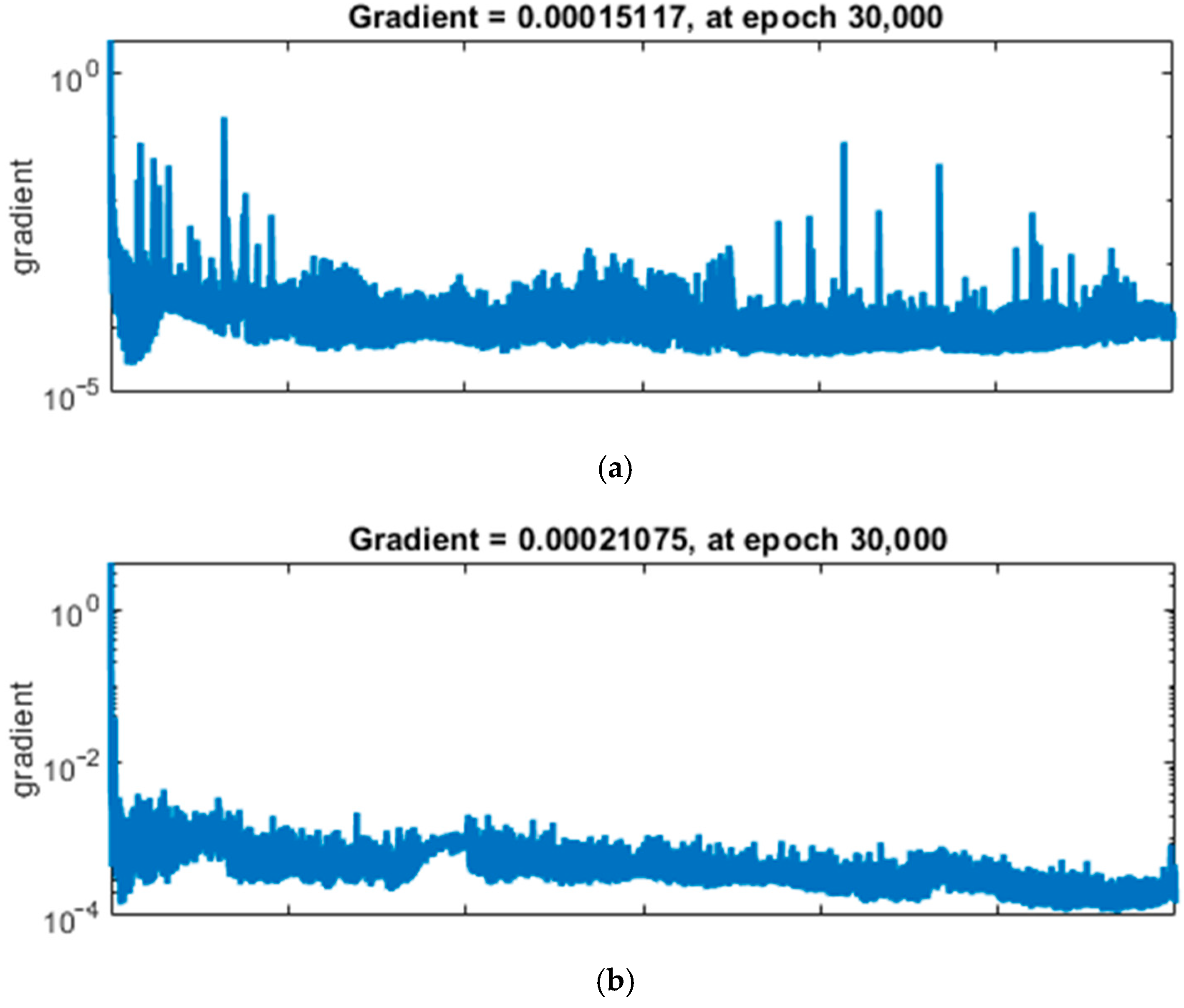
The training process visualizations for the two ANN MLP models demonstrate the behavior of the gradient descent algorithm over 30,000 epochs (see Figure 2). The gradient, representing the optimization algorithm’s step size in adjusting network weights, diminishes over time in both figures, suggesting convergence toward a local minimum. The blue plots display the gradient values on a logarithmic scale, which helps to identify changes over several orders of magnitude. It can be seen that the gradient for the “freight cost” model steadily decreases to a final value of 0.00015117, indicating that the weights are approaching optimal values that minimize prediction error. In the lower subplot representing validation checks, there is a flat line at zero, indicating that no early stopping occurred, and the validation performance did not deteriorate throughout training. Additionally, the “delivery time” model exhibits a final gradient of 0.00021075, indicating a successful training phase. Validation checks show no upward spikes, indicating that the model did not experience overfitting and its performance on the validation set remained stable.
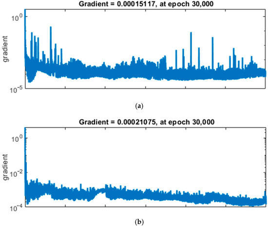
Figure 2.
Convergence of ANN training gradients for (a) “freight cost” and (b) “delivery time” models over 30,000 epochs, displaying the final gradients at the conclusion of training.
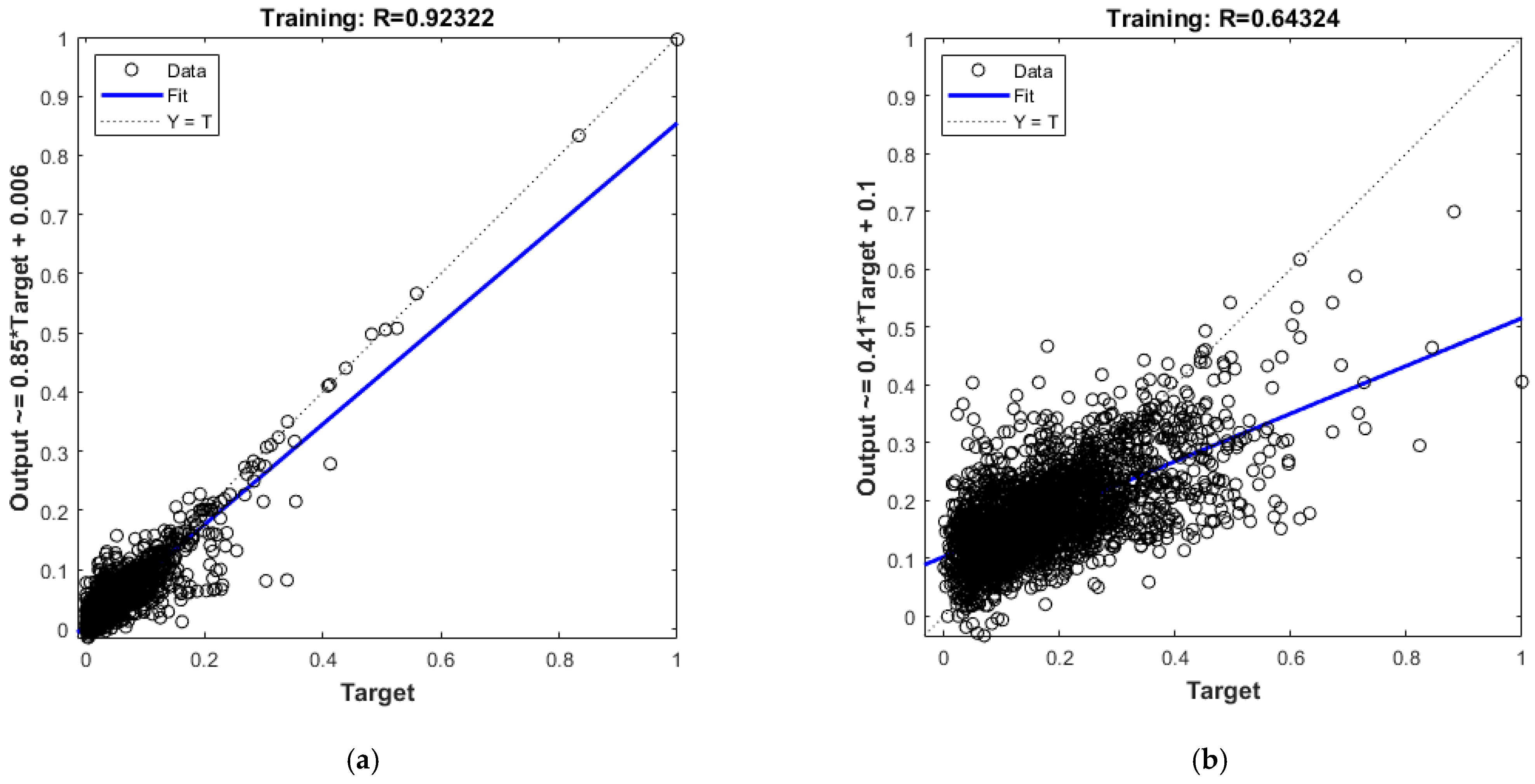
Figure 3 illustrate the correlation between the targets and the outputs of the trained neural network models, providing insight into the predictive performance of the models. In the first scatter plot, the “freight cost” model demonstrates a strong correlation between predicted and actual values, with a high correlation coefficient (R) of 0.92322. The data points are closely clustered around the line of perfect fit (Y = T), indicating a high level of predictive accuracy. This suggests that the model effectively captures the underlying patterns in the data, making accurate predictions for freight cost with minimal error. Such strong performance underscores the robustness of the model in handling this specific target variable.
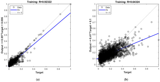
Figure 3.
Performance of ANN models during training, represented by regression plots comparing predicted outputs versus targets for (a) “freight cost” model with a high correlation (R = 0.92) and (b) “delivery time” model with a moderate correlation (R = 0.64).
Conversely, the second scatter plot reveals a weaker correlation between the predicted outputs and actual results for the “delivery time” model, with a significantly lower correlation coefficient (R) of 0.64324. In this case, the data points exhibit greater dispersion around the line of perfect fit, reflecting a less accurate predictive capability. The broader spread suggests that the model struggles to generalize well for this variable, potentially due to the higher complexity of the “delivery time” data or the presence of more noise and variability in the dataset. This finding highlights the need for further refinement of this model, possibly by incorporating additional features, fine-tuning hyperparameters, or applying advanced techniques to reduce noise and improve learning. Understanding these differences in performance is crucial for identifying areas where the models excel and where additional development is required to enhance predictive reliability.
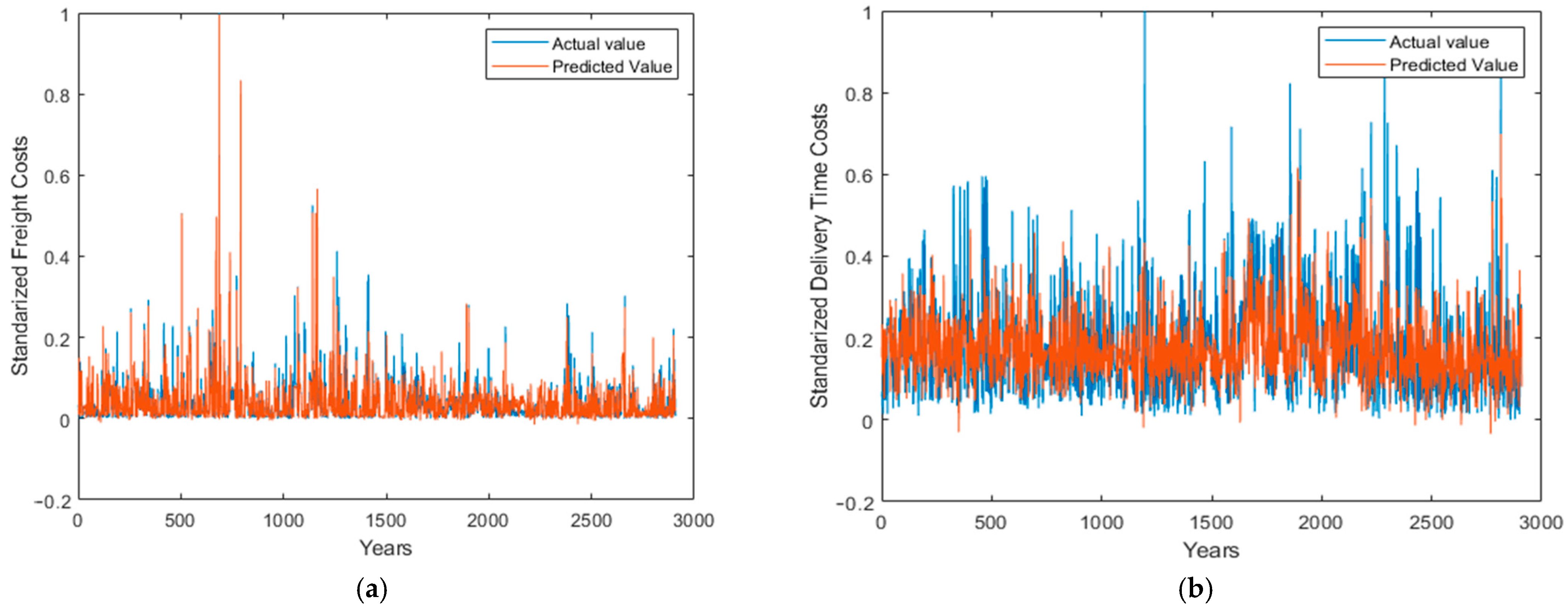
In the “freight cost” model, the alignment between actual and predicted lines indicates that the model accurately captures the variation in freight costs. As a result of this congruence, the model can be used to estimate freight costs during the supply chain optimization process, demonstrating its reliability. While there is a wider spread between the actual and predicted delivery times in the “delivery time” model, it still indicates an acceptable level of prediction accuracy. While it may not capture all peaks and troughs of delivery times precisely, this model provides a solid baseline prediction. Combined with other optimization techniques or when additional nuanced factors are considered, this model may be valuable. As a result of their respective predictive strengths, both models provide a substantial foundation for improving decision-making in the HIV drug supply chain (see Figure 4).
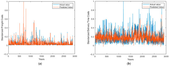
Figure 4.
Overlay of actual and predicted values for (a) standardized “freight cost” and (b) standardized “delivery time” across almost 3000 observations, showcasing the predictive accuracy of the ANN models.
4.2. Optimization of Freight Cost and Delivery Time
To optimize the HIV drug supply chain, we focused on minimizing the combined metrics of “freight cost” (f1) and “delivery time” (f’). The objective function aims to maximize both the economic and temporal efficiency of the supply chain. The optimization constraints were determined based on the requirement that the design variables must be positive and exceed α = 10% of their respective average values across the dataset. As a result, the solutions are feasible and significant in the context of the existing data. As a result, the constraints for the design variables “LineItemQuantity”, “PackPrice”, “UnitofMeasure”, and “weight” can be expressed mathematically as follows:
where denotes the average value of that variable across the entire dataset. The standardized forms of these variables, which were scaled to lie between 0 and 1 for the ANN modeling phase, were subsequently used as inputs for the optimization algorithm. The objective function to be minimized was defined as Equation (2). Where f1 represents the standardized “freight cost”, and f2 represents the standardized “delivery time”. The function encapsulates the essence of the optimization goal, which is to reduce the cost and time of deliveries concurrently. The Fmincon function in MATLAB was employed for optimization, utilizing the “active-set” algorithm. This algorithm is particularly well-suited for dealing with problems that have a mix of bound constraints and linear constraints. The optimization options were meticulously set to fine-tune the performance of the algorithm, with “ScaleProblem” configured to “obj-and-constr” to normalize the scale of the objective function and constraints, “ConstraintTolerance” set to a stringent 1 × 10⁻⁷ to ensure a precise adherence to the constraints, and “DiffMinChange”s adjusted to 1 × 10⁻⁶ to control the minimum change in variables for the finite-difference gradients. Based on these methods and settings, the optimal standardized values for “LineItemQuantity”, “PackPrice”, “UnitofMeasur”, and “weight” were found to be the following:
LineItemQuantity opt = 0.892
PackPrice opt = 0.903
UnitofMeasure opt = 0.101
Weight opt = 0.250
The de-standardization process, which converts these values back to their original scales, yielded the following optimum non-standardized values:
LineItemQuantity opt (originalscale) = 459,228.715
PackPrice opt (originalscale) = 1129.273 USD
UnitofMeasure opt (originalscale) = 101
Weight opt (originalscale) = 38,758.858 Kg
These values are instrumental in achieving the optimized “freight cost” and “delivery time”. The application of the optimized variables led to the following results:
FreightCost opt = 45,151.927 USD
DeliveryTime opt = 106.152 days
In our optimization framework, the constraints were carefully designed to ensure practical relevance and feasibility in real-world scenarios. Specifically, the constraints required that all design variables—Line Item Quantity, Pack Price, Unit of Measure (Per Pack), and Weight (Kilograms)—remain positive and exceed of their respective average values across the dataset. Mathematically, these constraints were expressed as follows:
These constraints reflect the realities of supply chain logistics, ensuring that the optimization solutions remain realistic. For example, Line Item Quantity cannot drop below a practical minimum threshold without jeopardizing supply chain efficiency, while Pack Price must account for the minimum cost viability set by suppliers. Similarly, constraints on weight ensure that shipment volumes remain feasible for transportation modes.
According to the results, the optimized design variables are capable of resulting in substantial cost savings and efficiency improvements compared to the initial supply chain state. The study’s results demonstrate the power of combining ANN predictive models with optimization algorithms to address complex supply chain challenges. In addition to providing insight into the factors affecting “freight cost” and “delivery time”, the models also assist in the optimization process in order to discover feasible and efficient solutions. Moreover, these findings underscore the broader applicability of ANN-driven optimization frameworks in tackling complex supply chain challenges. The approach not only enhances operational efficiency but also provides a systematic method to balance competing objectives, such as cost minimization and timely delivery. The use of MATLAB’s Fmincon with a carefully configured “active-set” algorithm ensures precise adherence to constraints and fine-tuning of results, making the methodology robust and scalable. Future research can build on this foundation by integrating additional factors, such as supplier reliability, geopolitical risks, and environmental considerations, to further optimize supply chain operations. These results reaffirm the critical role of advanced predictive and optimization tools in supporting decision-making, ensuring the sustainable delivery of essential resources like HIV drugs in challenging and dynamic environments. The predictive accuracy of the ANN models was evaluated using additional metrics to provide a more comprehensive assessment. For the “freight cost” model, the following performance metrics were recorded: RMSE = 0.045; MAE = 0.032; and R2 = 0.923, indicating strong predictive accuracy and alignment with the actual values. The scatter plot confirms this, with data points closely clustered around the line of perfect fit, validating the model’s robustness in predicting freight costs.
Conversely, the “delivery time” model exhibited comparatively lower accuracy, with RMSE = 0.089, MAE = 0.065, and R2 = 0.643. These metrics suggest that this model struggled to capture the variability inherent in delivery times, potentially due to unmodeled external factors such as weather conditions, political stability, and logistical constraints. The broader dispersion of data points in the scatter plot further highlights these limitations. To improve the “delivery time” model’s accuracy, we propose the incorporation of additional features that reflect real-world variability. Sensitivity analysis on key variables, such as “Shipment Mode” and “Vendor INCO Term”, will also be conducted to assess their relative influence on delivery time predictions. These enhancements aim to refine the model’s predictive capability and address the current limitations.
The comparative analysis confirms that Fmincon balances computational efficiency and solution precision, making it an ideal choice for the healthcare supply chain optimization problem. While EAs are effective for highly complex problems, their computational cost and stochastic variability make them less suitable for scenarios requiring fast, reliable results. LP, on the other hand, is not a viable alternative for the nonlinear nature of this problem. This robust benchmarking demonstrates that our proposed approach offers a practical and scalable solution for dual-objective optimization, achieving meaningful improvements in freight cost and delivery time while maintaining computational efficiency. Future work can extend this comparison to other advanced techniques, such as hybrid optimization frameworks, to further validate our methodology.
Table 3 compares the proposed Fmincon-based optimization approach against baseline methods, including linear programming (LP) and evolutionary algorithms (EAs), highlighting differences in optimization type, computational efficiency, convergence behavior, interpretability, performance metrics, and practical applicability.
Table 3.
Comparison of Fmincon, linear programming (LP), and evolutionary algorithms (EAs) on optimization type, efficiency, convergence, and performance.
5. Conclusions
This study leverages Artificial Neural Networks (ANNs) with a Multi-Layer Perceptron (MLP) architecture alongside the Fmincon optimization algorithm to enhance the efficiency of the HIV drug supply chain. The primary objective was to minimize two critical metrics: “freight cost’ and “delivery time”, which are vital to ensuring both cost-effectiveness and timely delivery in drug distribution systems. This methodology involved training ANN models in predicting these metrics based on four key design variables: “Line Item Quantity”, “Pack Price”, “Unit of Measure (Per Pack)”, and “Weight (Kilograms)”. Using a dataset comprising 10,325 cases that encapsulated diverse supply chain components, the models underwent rigorous training. The application of the gradient descent algorithm resulted in substantial improvements in prediction accuracy, effectively minimizing the error between predicted and actual values. Once validated, the ANN models were integrated into an optimization framework where constraints ensured that design variables remained within realistic bounds, such as exceeding 10% of their respective average values. The Fmincon algorithm was selected for its ability to handle complex constraints effectively, and its configuration was fine-tuned for precision. The optimization results, after de-standardizing the design variables, revealed significant improvements, with the optimized “freight cost” reduced to USD 45,151.93 and “delivery time” shortened to 106.15 days compared to baseline values.
These results underscore the transformative potential of machine learning and optimization techniques in addressing challenges within complex supply chains. Optimizing the HIV drug supply chain yields not only economic benefits but also profound social impacts. By reducing delivery times, critical medications can be made available more promptly, improving health outcomes and enhancing the quality of life for patients. Additionally, cost savings from reduced freight expenses can be reallocated to other essential areas, such as medical research, infrastructure development, and expanding healthcare access. This study also highlights the robustness and adaptability of combining ANNs with optimization algorithms, providing a scalable approach for various industries. However, limitations were identified, particularly regarding the accuracy of the “delivery time” predictions, which suggests that additional variables—such as weather conditions, geopolitical factors, or global health crises—could further refine this model. Future research should explore incorporating such granular data to address these complexities and improve predictive accuracy. This work bridges the gap between healthcare, supply chain management, and data science, illustrating how interdisciplinary approaches can tackle real-world challenges. Beyond healthcare, this methodology has implications for manufacturing, retail, and logistics sectors, demonstrating the versatility of data-driven, analytical solutions. The success of this study reaffirms the value of innovative approaches in supply chain optimization, emphasizing the need for continued research to refine models and drive positive economic and societal outcomes.
6. Future Work
To expand the future research section, we will include the potential of multi-objective evolutionary algorithms, such as NSGA-II or MOEA/D, to explore a broader solution space and address the trade-offs between freight cost and delivery time more effectively. Additionally, we will propose developing real-time supply chain optimization frameworks that leverage dynamic data, such as real-time tracking, weather conditions, and geopolitical factors, to enhance adaptability and decision-making. These directions will provide a foundation for extending the applicability and robustness of the proposed approach.
Author Contributions
Conceptualization, A.G., B.F. and J.F.; Methodology, A.G. and B.F.; Software, A.G. and B.F.; Validation, A.G., B.F. and J.F.; Formal analysis, B.F. and J.F.; Investigation, A.G.; Writing—original draft, A.G.; Writing—review & editing, A.G., B.F. and J.F.; Visualization, A.G.; Supervision, B.F. and J.F.; Project administration, B.F. and J.F.; Funding acquisition, B.F. All authors have read and agreed to the published version of the manuscript.
Funding
This research was funded by the National Social Science Fund of China project: Research on the Modernization of Intellectual Property Governance for Digital Innovation (22VRC064) to Bo Feng.
Institutional Review Board Statement
Not applicable.
Data Availability Statement
The data are available upon request to the corresponding author.
Conflicts of Interest
Authors have no conflicts of interest.
References
- Barrow, G.J.; Fairley, M.; Brandeau, M.L. Optimizing interventions across the HIV care continuum: A case study using process improvement analysis. Oper. Res. Health Care 2020, 25, 100258. [Google Scholar] [CrossRef] [PubMed]
- Alemnji, G.; Peter, T.; Vojnov, L.; Alexander, H.; Zeh, C.; Cohn, J.; Watts, D.H.; de Lussigny, S. Building and sustaining optimized diagnostic networks to scale-up HIV viral load and early infant diagnosis. JAIDS J. Acquir. Immune Defic. Syndr. 2020, 84, S56–S62. [Google Scholar] [CrossRef] [PubMed]
- Larson, C.; Burn, R.; Minnick-Sakal, A.; Douglas, M.O.K.; Kuritsky, J. Strategies to reduce risks in ARV supply chains in the developing world. Glob. Health Sci. Pract. 2014, 2, 395–402. [Google Scholar] [CrossRef]
- Ripin, D.J.; Jamieson, D.; Meyers, A.; Warty, U.; Dain, M.; Khamsi, C. Antiretroviral procurement and supply chain management. Antivir Ther. 2014, 19 (Suppl. 3), 79–89. [Google Scholar] [CrossRef] [PubMed]
- Rojo, P.; Carpenter, D.; Venter, F.; Turkova, A.; Penazzato, M. The HIV drug optimization agenda: Promoting standards for earlier investigation and approvals of antiretroviral drugs for use in adolescents living with HIV. J. Int. AIDS Soc. 2020, 23, e25576. [Google Scholar] [CrossRef] [PubMed]
- Cao, E.P. Decision Making in the HIV/AIDS Supply Chain. Ph.D. Thesis, Massachusetts Institute of Technology, Cambridge, MA, USA, 2007. [Google Scholar]
- Schouten, E.J.; Jahn, A.; Ben-Smith, A.; Makombe, S.D.; Harries, A.D.; Aboagye-Nyame, F.; Chimbwandira, F. Antiretroviral drug supply challenges in the era of scaling up ART in Malawi. J. Int. AIDS Soc. 2011, 14, S4. [Google Scholar] [CrossRef] [PubMed]
- Stulens, S.; De Boeck, K.; Vandaele, N. HIV supply chains in low-and middle-income countries: Overview and research opportunities. J. Humanit. Logist. Supply Chain. Manag. 2021, 11, 369–401. [Google Scholar] [CrossRef]
- Jónasson, J.O.; Deo, S.; Gallien, J. Improving HIV early infant diagnosis supply chains in sub-Saharan Africa: Models and application to Mozambique. Oper. Res. 2017, 65, 1479–1493. [Google Scholar] [CrossRef]
- Pastakia, S.D.; Tran, D.N.; Manji, I.; Wells, C.; Kinderknecht, K.; Ferris, R. Building reliable supply chains for noncommunicable disease commodities: Lessons learned from HIV and evidence needs. Aids 2018, 32, S55–S61. [Google Scholar] [CrossRef]
- Ahmad, F.; Alnowibet, K.A.; Alrasheedi, A.F.; Adhami, A.Y. A multi-objective model for optimizing the socio-economic performance of a pharmaceutical supply chain. Socio-Econ. Plan. Sci. 2022, 79, 101126. [Google Scholar] [CrossRef]
- Olutuase, V.O.; Iwu-Jaja, C.J.; Akuoko, C.P.; Adewuyi, E.O.; Khanal, V. Medicines and vaccines supply chains challenges in Nigeria: A scoping review. BMC Public Health 2022, 22, 11. [Google Scholar] [CrossRef]
- Lugada, E.; Komakech, H.; Ochola, I.; Mwebaze, S.; Olowo Oteba, M.; Okidi Ladwar, D. Health supply chain system in Uganda: Current issues, structure, performance, and implications for systems strengthening. J. Pharm. Policy Pract. 2022, 15, 14. [Google Scholar] [CrossRef]
- Torrado, A.; Barbosa-Póvoa, A. Towards an optimized and sustainable blood supply chain network under uncertainty: A literature review. Clean. Logist. Supply Chain 2022, 3, 100028. [Google Scholar] [CrossRef]
- Madani Saatchi, H.; Arshadi Khamseh, A.; Tavakkoli-Moghaddam, R. Solving a new bi-objective model for relief logistics in a humanitarian supply chain by bi-objective meta-heuristic algorithms. Sci. Iran. 2021, 28, 2948–2971. [Google Scholar]
- Tat, R.; Heydari, J.; Rabbani, M. A mathematical model for pharmaceutical supply chain coordination: Reselling medicines in an alternative market. J. Clean. Prod. 2020, 268, 121897. [Google Scholar] [CrossRef]
- Ávila-Ríos, S.; Parkin, N.; Swanstrom, R.; Paredes, R.; Shafer, R.; Ji, H.; Kantor, R. Next-generation sequencing for HIV drug resistance testing: Laboratory, clinical, and implementation considerations. Viruses 2020, 12, 617. [Google Scholar] [CrossRef]
- Siddiqui, R.; Azmat, M.; Ahmed, S.; Kummer, S. A hybrid demand forecasting model for greater forecasting accuracy: The case of the pharmaceutical industry. Supply Chain. Forum Int. J. 2022, 23, 124–134. [Google Scholar] [CrossRef]
- Sindhwani, R.; Jayaram, J.; Saddikuti, V. Ripple effect mitigation capabilities of a hub and spoke distribution network: An empirical analysis of pharmaceutical supply chains in India. Int. J. Prod. Res. 2023, 61, 2795–2827. [Google Scholar] [CrossRef]
- Singh, S.; Kumar, R.; Panchal, R.; Tiwari, M.K. Impact of COVID-19 on logistics systems and disruptions in food supply chain. Int. J. Prod. Res. 2021, 59, 1993–2008. [Google Scholar] [CrossRef]
- Jamieson, D.; Kellerman, S.E. The 90 90 90 strategy to end the HIV Pandemic by 2030: Can the supply chain handle it? J. Int. AIDS Soc. 2016, 19, 20917. [Google Scholar] [CrossRef] [PubMed]
- Xiong, W.; Hupert, N.; Hollingsworth, E.B.; O’Brien, M.E.; Fast, J.; Rodriguez, W.R. Can modeling of HIV treatment processes improve outcomes? Capitalizing on an operations research approach to the global pandemic. BMC Health Serv. Res. 2008, 8, 166. [Google Scholar] [CrossRef]
- Enyinda, C.I.; Dunu, E.S.; Hawkins, A. Improving HIV/AIDS Healthcare Supply Chain in Sub-Saharan Africa Through New Partnership for Supply Chain Management. J. Glob. Bus. Issues 2009, 3, 95–103. [Google Scholar]
- Rahimi, M.; Al Masry, Z.; Templeton, J.M.; Schneider, S.; Poellabauer, C. A Comprehensive Multifunctional Approach for Measuring Parkinson’s Disease Severity. Appl. Clin. Inform. 2025, 16, 011–023. [Google Scholar] [CrossRef]
- Ogunsoto, O.V.; Olivares-Aguila, J.; ElMaraghy, W. A conceptual digital twin framework for supply chain recovery and resilience. Supply Chain. Anal. 2025, 9, 100091. [Google Scholar] [CrossRef]
- Strika, Z.; Petkovic, K.; Likic, R.; Batenburg, R. Bridging healthcare gaps: A scoping review on the role of artificial intelligence, deep learning, and large language models in alleviating problems in medical deserts. Postgrad. Med. J. 2024, 101, 4–16. [Google Scholar] [CrossRef] [PubMed]
- Jones, E.; Azeem, G.; Erick, C.J.I.; Felicia, J. Impacting at risk communities using AI to optimize the COVID-19 pandemic therapeutics supply chain. Int. Supply Chain. Technol. J. 2020, 6, 2. [Google Scholar] [CrossRef]
- Bhargavi, V.S.; Sawai, N.M.; Chakravarthi, M.K.; Mankar, A.R.; Rodriguez, M.A.M.; Pavitha, N. Enhancing Supply Chain Traceability and Transparency Through Machine Learning Implementation. In Interdisciplinary Approaches to AI, Internet of Everything, and Machine Learning; IGI Global Scientific Publishing: Hershey, PA, USA, 2025; pp. 437–450. [Google Scholar]
- Riad, M.; Naimi, M.; Okar, C. Enhancing Supply Chain Resilience Through Artificial Intelligence: Developing a Comprehensive Conceptual Framework for AI Implementation and Supply Chain Optimization. Logistics 2024, 8, 111. [Google Scholar] [CrossRef]
- Dongare, A.D.; Kharde, R.R.; Kachare, A.D. Introduction to artificial neural network. Int. J. Eng. Innov. Technol. (IJEIT) 2012, 2, 189–194. [Google Scholar]
Disclaimer/Publisher’s Note: The statements, opinions and data contained in all publications are solely those of the individual author(s) and contributor(s) and not of MDPI and/or the editor(s). MDPI and/or the editor(s) disclaim responsibility for any injury to people or property resulting from any ideas, methods, instructions or products referred to in the content. |
© 2025 by the authors. Licensee MDPI, Basel, Switzerland. This article is an open access article distributed under the terms and conditions of the Creative Commons Attribution (CC BY) license (https://creativecommons.org/licenses/by/4.0/).