Abstract
In the context of big data and artificial intelligence, analyzing and extracting actionable insights from extensive datasets to enhance decision-making processes presents both intriguing opportunities and formidable challenges. Existing multiple criteria sorting (MCS) methodologies often struggle with the magnitude of these datasets, particularly in terms of time and memory requirements. Furthermore, traditional approaches typically rely on direct preference information, which can be cognitively demanding for decision-makers and may not scale effectively with increasing data complexity. This study introduces a scalable MCS approach grounded in the MapReduce framework, designed to handle extensive sets of alternatives and preference information in a parallel processing paradigm. The proposed approach utilizes an additive piecewise-linear value function as the underlying preference model, with model parameters inferred from assignment examples on a subset of reference alternatives through the application of preference disaggregation principles. To enable the parallel execution of the sorting procedure, a convex optimization model is formulated to estimate the parameters of the preference model. Subsequently, a parallel algorithm is devised to solve this optimization model, leveraging the MapReduce framework to process the set of reference alternatives and associated preference information concurrently, thereby accelerating computational efficiency. Additionally, the performance of the proposed approach is evaluated using a real-world dataset and a series of synthetic datasets comprising up to 400,000 alternatives. The findings demonstrate that this approach effectively addresses the MCS problem in the context of large sets of alternatives and extensive preference information.
1. Introduction
The goal of multiple criteria decision aiding (MCDA) is to support a decision maker (DM) in choosing a subset of alternatives that are judged as the most satisfactory from the whole set, or ranking alternatives from the best to the worst in a preference pre-order, or assigning all alternatives to predefined and preferentially ordered categories [1,2,3]. The above types of problems are referred to as choice, ranking, and sorting, respectively [4,5]. Refs. [6,7] provided comprehensive reviews of MCDA approaches in the literature for dealing with various decision scenarios, and reported new trends and recent developments from the last several years.
In this paper, we focus on the MCS problem. The MCS problem is of major practical interest in many domains, such as supply chain management [8], ecological planning [9], renewable energy [10], and education [11]. Like the choice and ranking problems, the MCS problem requires the DM to provide preference information in either a direct or indirect manner. In the direct case, the DM is guided by an analyst to specify the parameters of the preference model that could be either precise values for or constraints on weights, trade-offs, category profiles and so on [12]. Such an elicitation process is usually structured as a series of interactive communication sessions in which the analyst guides the DM to express preferences progressively. Thus, the willingness of the DM to cooperate with the analyst and the ability of the analyst to elicit preference information from the DM strongly influences of the success of this approach [13]. On the other hand, in the indirect case the DM is required to provide a set of assignment examples on reference alternatives, which could either come from the DM’s previous decisions, or specified by the DM on a subset of alternatives under consideration. Such indirect preference information is usually utilized along with the preference disaggregation analysis, which is a general methodological framework for constructing a preference model that is as consistent as possible with the assignment examples provided by the DM [14]. The constructed preference model is applied to new decision instances to arrive at an assignment recommendation. MCS approaches that utilize indirect preference information and the preference disaggregation paradigm are regarded to be more user-friendly to the DM than methods based on direct preference information, because the former reduces the cognitive effort for the DM during the course of providing preference information [14].
Recent developments in information technology have resulted in an explosive growth in data gathered from various fields. Ninety percent of the data in the world has been created in the last two years, at a rate of 2.5 quintillion bytes on a daily basis. This is commonly referred to as big data1. Retrieving useful information and knowledge from big data can enable organizations to reach better decisions, including deepening customer engagement, optimizing operations, preventing threats and fraud, and capitalizing on new sources of revenue. An estimated 89 percent of enterprises believe that those who do not take advantage of big data analytics run the risk of losing a competitive edge in the market2, and thus they are gearing up to leverage their information assets to gain a competitive advantage. MCS is also gaining importance in the era of big data, because it can help firms, organizations, and governments to reach better data-driven decisions. For example, in the field of finance, a rating agency can adopt MCS approaches to evaluate the credit risks of thousands of firms, and assign a credit rating to each firm [15,16,17]. As another example, in the field of e-business, firms can utilize big data analytics to analyze the preferences of a large population of consumers, and then apply MCS approaches to divide a large market into segments in order to tailor different marketing policies for targeted segments [18,19].
However, it is challenging for existing MCS methods to deal with problems that contain a large set of alternatives and massive preference information. In fact, most MCS methods were originally designed to address problems with several dozen alternatives. The scalability to different problem sizes is not at the core of such approaches [14]. More specifically, for MCS methods based on the preference disaggregation paradigm, the construction of a preference model from a set of assignment examples usually involves linear programming (LP) and integer programming (IP) formulations. LP models are usually employed to minimize the sum or the maximum of real-valued error variables that represent the degrees of violations of preference relations. IP formulations are used to minimize the number of deviations between the actual evaluation of the DM on the reference alternatives and the recommendations of the inferred preference model [13,20]. To the best of our knowledge, all LP and IP formulations in existing MCS methods require the data to fit into the operational memory. Such requirement stems from the fact that most LP or IP solvers search for the optimal solution in the operational memory of a computer and thus the constraint matrix must be loaded in advance. This exceeds the processing capabilities of existing MCS methods in terms of the memory consumption and/or the computational time when dealing with huge amounts of data. Thus, new techniques must be introduced to redesign existing MCS methods so that they can scale up well with new storage and time requirements.
In this study, we aim to propose a new MCS approach for addressing a large set of alternatives and massive preference information. The preference information refers to assignment examples on reference alternatives, which may come from past decision examples, such as historical credit ratings of firms or past customer segmentation during a certain period. In order to deal with such large-scale data sets efficiently, the proposed approach is implemented with the MapReduce framework in a parallel manner. MapReduce is a popular parallel computing paradigm, which is designed to process large-scale data sets. It divides the original data set into disjoint splits, each of which can be easily handled by a single working node. Then, the intermediate solutions from different subsets are aggregated in some way to obtain the final outcomes. Such a computing paradigm allows us to parallelize applications on a computer cluster in a highly scalable manner.
Note that the decision scenario considered in this study is slightly different from those encountered by most traditional MCS methods. In traditional research, constructing a preference model based on the preference disaggregation paradigm is implemented in an interactive procedure where the DM, with the assist of the analyst, could provide assignment examples incrementally so that the DM will calibrate the constructed preference model progressively [14]. However, in this study, we assume that the assignment examples come from past decision examples, and aim to infer a preference model from such preference information directly and then apply the constructed preference model to new decision alternatives. Therefore, we need a new method for constructing a preference information in an automatic way without the participation of the DM. Such a constructed preference model should be not only consistent with the provided assignment examples, but also robust in the sense that it can tolerate the imperfection in the considered data sets since we care about the predictive ability of the preference model on new decision alternatives.
In this proposed approach, we employ an additive piecewise-linear value function as the preference model, and infer the model’s parameters from the assignment examples using the preference disaggregation paradigm. According to the principle of assignment consistency, we propose a convex optimization model to derive a preference model that can restore the preference information as consistently as possible. This optimization model uses the Sigmoid function to measure the degree of inconsistency when the assignment of any pair of reference alternatives that violates the consistency principle and the margin to the decision boundary when the assignment of accords the consistency principle, thus ensuring the derived value function model being both consistent and robust. In contrast to traditional MCS methods, this optimization model avoids using slack variables to specify the degree of inconsistency for any assignment example and does not translate preference information to the linear constraints of the optimization model. Thus, it is especially suitable for addressing large-scale data sets since it does not need to load a huge constraint matrix into the operational memory. In order to solve the optimization model efficiently, we implement the Zoutendijk’s feasible direction method [21] with the MapReduce framework. The algorithm iteratively searches for the optimal solution by checking a direction that is both feasible and descent. During the iterative process, the MapReduce framework is used to accelerate calculating the value of the objective function at the current solution and its gradient in a parallel manner.
We summarize the contributions of our work from the following aspects. First, our work represents a new MCS approach implemented with the MapReduce framework to address a large set of alternatives and massive preference information. Although data-driven decision making has become a popular contemporary subject, no previous methods can deal efficiently with such a MCS problem. Our approach displays high scalability and an ability to tackle the MCS problem with a large set of alternatives and massive preference information. Second, we propose a convex optimization model to derive a preference model, which answers to consistency and robustness concerns simultaneously. Differently from traditional techniques, this optimization model avoids using slack variables to specify the degree of inconsistency for any assignment example and thus contains a relatively small set of variables and linear constraints, which is especially suitable for addressing large-scale MCS problems. Finally, we propose a parallel method to solve the developed optimization model efficiently. This parallel method does not need to load the whole data set into the main memory and thus has no specific requirements regarding the processing capabilities of working nodes. It proceeds by scanning the preference information sequentially, which is beneficial for the parallel implementation with the MapReduce framework to accelerate the computation. Moreover, it is robust to the splitting and combining operations in the MapReduce framework and the final results are irrelevant for the parallel implementation.
This paper is an extended version of the paper submitted to the DA2PL 2018 conference (From Multiple Criteria Decision Aid to Preference Learning) [12]. In original paper, we proposed the prototype of the developed scalable decision-making approach and discussed its basic properties. In this paper, the extensions include: (a) a generalized formulation of the problem space, (b) comprehensive performance evaluation across different problem settings, and (c) formal complexity analysis of the proposed approach.
We organize the remainder of the paper in the following way. Section 2 provides a literature review on MCS methods based on indirect preference information and the preference disaggregation paradigm. In Section 3, we describe the proposed approach to deal with the MCS problem with a large set of alternatives and massive preference information, as well as its MapReduce implementation. In Section 4, we apply the proposed approach to a real-word data set and compare the results to that of the UTADIS method. Section 5 presents and discusses the experimental results of applying the proposed approach to artificially generated data. Section 6 concludes the paper and provides discussion for future research.
2. Literature Review
The MCS problem has attracted significant interest over the past decade, and various MCS approaches have been proposed in the literature [22,23]. According to the employed preference model, which reflects the value system of the DM, MCS approaches in the literature can be categorized into three types: (1) methods motivated by value functions, such as the UTADIS method and its variants [5,24,25,26,27,28]; (2) methods based on outranking relations, such as the ELECTRI Tri-B methods [29,30,31,32], ELECTRI Tri-C methods [33,34], ELECTRI-based methods [35,36] and PROMETHEE-based methods [36,37]; and (3) rule induction-oriented procedures, such as the DRSA method and its extensions [38,39].
Because the approach proposed in this paper belongs to the class of methods based on indirect preference information and the preference disaggregation paradigm, let us review the development of this family of MCS methods as follows. First of all, we focus on value-driven soring methods. The earliest study in this line originates from the UTADIS method [24,40]. Based on a set of assignment examples provided by the DM, UTADIS aims to estimate an additive value function, as well as comprehensive value thresholds separating consecutive categories, with the minimum misclassification error. For each assignment example on a particular reference alternative, UTADIS introduces two slack variables to measure the differences between the reference alternative’s comprehensive value and the upper and lower value thresholds that delimit the corresponding category. Then, UTADIS organizes all assignment examples as linear constraints and uses the LP technique to minimize the sum of slack variables for all assignment examples. The constructed preference model with the minimal sum of misclassification errors is applied to assign a non-reference alternative by comparing its comprehensive value to the estimated value thresholds. Another representative among the MCS methods in this line is the MHDIS method [24]. Differently from UTADIS, the MHDIS method employs a sequential/hierarchical process to perform the assignment decision. It uses several LP and IP models to construct a value function model from assignment examples by minimizing the total number of misclassifications as well as maximizing the clarity of correct classification. From the last decade, the methodology of Robust Ordinal Regression (ROR) has been prevailing in the MCDA community. The methods in the family of ROR for sorting problems include UTADISGMS [5], UTADISGMS-GROUP [41] and MCHP for sorting [42]. These methods propose to consider the whole set of compatible instances of value functions and derive necessary and possible assignments for a non-reference alternative. Since the necessary and possible assignments are obtained from the whole set of compatible instances of value functions, it is necessary to obtain a consistent set of assignment examples from the DM. In case of inconsistency, it is usual to identify the inconsistent subset of assignment examples using IP formulations and require the DM to revise or remove them so as to restore consistency.
The second stream of MCS methods based on indirect preference information and the preference disaggregation paradigm are the ones based on outranking relations. Ref. [43] first applied the preference disaggregation analysis to infer the parameters (including criteria weights, category profiles and thresholds) of the ELECTRE TRI-B method [29] from the given assignment examples. One can refer to [30,31,44,45,46] for more methods utilizing various techniques that aim to infer the parameters of ELECTRE TRI-B from the assignment examples. Besides, Ref. [47] reformulated the ELECTRI Tri-C methods [33,34] and developed a disaggregation method for estimating a compatible outranking model from the provided preference information. Apart from the preference disaggregation approaches based on ELECTRE TRI-B and ELECTRE TRI-C, Ref. [35] proposed an assignment principle for outranking-based sorting and presented a disaggregation procedure to compare non-reference alternatives to reference ones and to assign them to categories accordingly. Ref. [36] extended the work of Ref. [35] and developed a method for robustness analysis within the framework of ROR. Due to the relational nature of outranking relations and the involvement of several thresholds related to each criterion, the above outranking-based preference disaggregation methods utilize the integer/non-linear programming techniques or evolutionary algorithms to infer the parameters of an outranking model from the given preference information.
When it comes to rule induction-oriented preference disaggregation procedures for sorting problems, let us mention the DRSA method [38], which aims to infer a preference model composed of a set of “if…, then…” decision rules from the assignment examples. DRSA utilizes a dominance relation for the rough approximation of categories and applies a rule induction strategy for representing the knowledge underlying the assignment examples and for performing the assignment of non-reference alternatives. Ref. [39] adapted the methodology of ROR to the rule-based preference model and provided for each non-reference alternative the necessary and possible assignments. Note that the complexity of generating decision rules from assignment examples is exponential and thus a considerable amount of computational time and operational memory is needed [39].
To sum up, the above MCS methods reveal the following two inherent features that are distinguished from other data analysis techniques (e.g., machine learning). The first one consists in the fact that the size of alternatives in MCS is usually limited to several dozens. The optimization techniques (including LP, IP, evolutionary algorithms, and so on) used in these methods can work out the optimal solutions in a reasonable time for small data sets. Thus, the computational efficiency is not the concern of such MCS methods. The second feature is the active participation of the DM. In most of such MCS methods, constructing a preference model is usually organized as interactive sessions in which the DM express their preferences in form of decision examples in order to calibrate the constructed model that would fit the DM’s preferences progressively. However, recall that the decision scenario considered in this study is different from those encountered by traditional MCS methods. When facing a large set of alternatives and massive preference information, traditional MCS methods cannot address the problem properly due to the limitation of computational time and operational memory. Moreover, without the participation of the DM, it is difficult for traditional MCS methods to derive a preference model that both fits decision examples well and has a good predictive ability on new decision alternatives. Thus, it is necessary to propose a new MCS approach for dealing with large-scale data sets and constructing a preference model from assignment examples in an automatic way without the participation of the DM.
3. Proposed Approach
3.1. Problem Description
The aim of this study is to classify a finite set of m alternatives … into p categories …, such that is preferred to (denoted by ), . Each alternative from set A has to be assigned to exactly one category. Such a classification decision is built on some preference information provided by the DM, which involves a set of assignment examples concerning a finite set of reference alternatives …}. Let be the cardinality of the reference set . An assignment example corresponds to the specified assignment of a reference alternative to a category . All the alternatives are evaluated in terms of n criteria …. The performance of on , , is denoted by . Without loss of generality, all the criteria are assumed to have a monotone increasing direction of preferences, i.e., either the greater or the less , the more preferred on , .
To perform the assignment of alternative , we shall use as the preference model an additive value function U of the following form:
where is the comprehensive value of a, and , , are marginal value functions for each criterion. Additive value functions are the most common preference model in MCDA due to their intuitive interpretation and relatively easy computation, despite the underlying assumption on the preferential independence of criteria and the compensation between criteria [48]. In many practical applications, this assumption is commonly adopted due to its ability to significantly reduce the complexity of the decision model. For instance, the UTADIS method, which is a well-established approach in multiple criteria sorting, also relies on this assumption to construct additive value functions. Our choice of an additive piecewise-linear value function is primarily motivated by the need to balance model complexity with computational efficiency, especially when dealing with large-scale datasets.
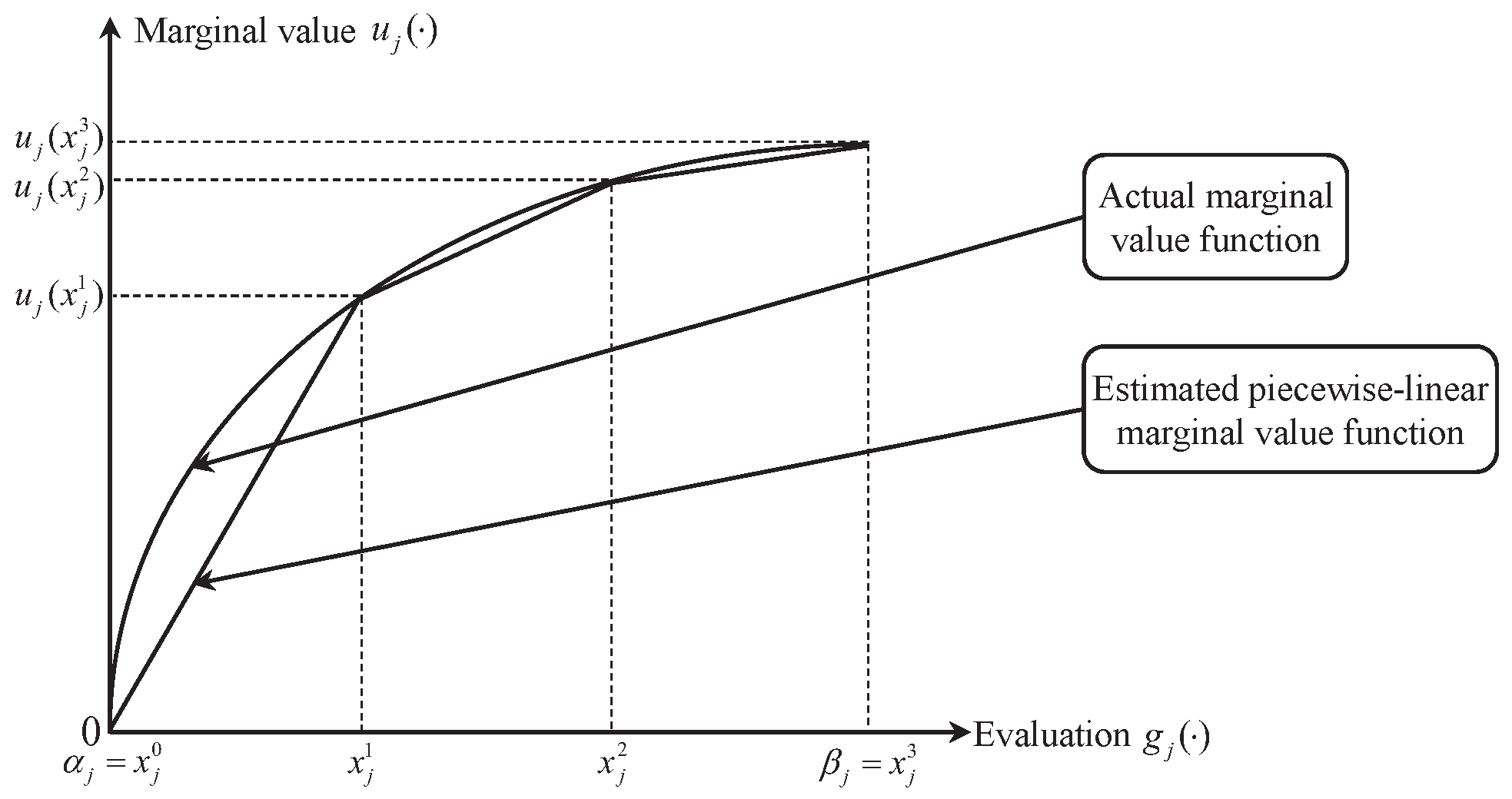
In this paper, a piecewise-linear function is used to estimate the actual value function of criterion , (see Figure 1). Let denote the evaluation scale of criterion , such that and are the minimal and maximal evaluation, respectively. In defining the piecewise-linear form of the marginal value function , is divided into equal sub-intervals , where , …. Then, we can use linear interpolation to estimate marginal values:
According to (1), we only need to determine the marginal values at characteristic points, so that the piecewise-linear value function can be fully specified. Note that when using piecewise-linear value functions with a sufficient number of characteristic points, we can approximate any non-linear value function. The latter observation enhances their appropriateness for a wide range of applications.

Figure 1.
Piecewise-linear form of marginal value function.
Then, we introduce a new variable to denote the difference between and :
Therefore, with the use of , can be formulated in the following way:
Definition 1 ([49]).
where satisfies for .
The characteristic vector of alternative a is a column vector of which entries are the coefficients of variables in marginal values on each criterion , , where
Having defined , we can compute comprehensive value as follows:
where . To normalize the value of alternative a such that , we can set
where is a column vector whose entries are all equal to 1. In this case, the trade-off weights for each criterion can be retrieved as , .
3.2. Model for Estimating Value Function
- In this paper, we perform the assignment of alternatives according their comprehensive values by considering the following consistency principle for assignment.
Definition 2.
For any pair of alternatives a and b, a given value function is said to be consistent with the assignment of a and b (denoted by and , respectively, and ), if and only if
where ≿ and ≾ mean “as least as good as” and “as most as good as”, respectively. Observe that (2) and (3) are equivalent to
since and .
For many MCS problems, we cannot find a consistent value function given a set of reference alternatives because of some inconsistent assignment examples. In this case, traditional methods based on the preference disaggregation paradigm introduce a set of slack variables, which would specify how much inconsistency there is for any pair of reference alternatives that violate the above consistency principle, and then minimize the sum of all the slack variables by solving a LP model to derive a value function that is as consistent with the preference information as possible. However, considering that a large-scale problem contains a huge number of reference alternatives, the number of linear constraints and that of slack variables in the objective of the LP model will be quite large, which exceeds the processing capabilities of most LP solvers. In this paper, differently from traditional methods, we propose a new model to estimate an additive value function as follows.
First, let us introduce a set of indicators for any pair of reference alternatives such that , which are defined as
According to the above consistency principle for assignment, we aim to find a vector such that, for any pair of reference alternatives with , we have
Then, instead of using slack variables, we can transform into a value for any pair of reference alternatives so that we can use the difference between and to measure the inconsistency. should satisfy the following conditions:
- (a) is monotone and increasing with respect to ,
- (b) is bounded with the interval ,
- (c) if ; if ; and if .
In this way, we can use the difference between and to measure (a) how much inconsistency there is for any pair of reference alternatives and that violate the consistency principle and (b) how much the margin to the decision boundary is when the assignment of accords the consistency principle. Specifically, for the case that , if the inconsistency occurs (i.e., ), the difference between and is greater than 0.5 because ; the greater the difference between and is, the larger the degree of consistency is for the assignment of and . On the contrary, if the assignment of accords the consistency principle (i.e., ), the difference between and is smaller than 0.5 because ; the smaller the difference between and is, the larger the margin to the decision boundary is for the assignment of and . The case that can be analyzed analogously. Therefore, we propose to minimize the difference between and so that we can derive a value function that will not only minimize the degree of inconsistency when the assignment of violates the consistency principle (i.e., consistency), but also maximize the margin to the decision boundary when the assignment of accords the consistency principle (i.e., robustness) so that the derived preference model will tolerate the imperfection in the considered data set.
In this paper, we use the following Sigmoid function to instantiate the function :
The Sigmoid function satisfies all the above requirements of the function . Then, we can consider the following non-linear optimization model to derive a value function that is as both consistent and robust as possible.
For any pair of reference alternatives , when , the above optimization model aims to maximize to minimize the difference between and and neglects the term because . On the contrary, when , the above optimization model attempts to maximize to minimize the difference between and and neglects the term because . Note that the objective (8) is in the multiplicative form, rather than the additive form, because the former avoids the compensation between different terms in the objective, which is especially useful when the number of pairs of reference alternatives is large. The most important benefit of choosing the Sigmoid function consists in that, by using the Sigmoid function, the optimization model (8)–(9) is a convex optimization problem because the objective (8) is convex which has been proved in [50]. This inspires us to extend classical convex optimization algorithms to address such a problem. Note that the objective (8) has been used in the logistic regression, a machine learning model for binary classification in the probabilistic framework [50]. One can observe that the optimization model (8)–(9) contains linear constraints and all the preference information is involved in the objective (8). In this way, we avoid loading a huge constraint matrix into the operational memory.
3.3. Algorithm Based on the MapReduce Framework
In order to solve the non-linear optimization model (8)–(9) for a large-scale problem efficiently, we propose a new parallel implementation for the Zoutendijk’s feasible direction method [21] based on the MapReduce framework. The Zoutendijk’s feasible direction method is an algorithm for solving constrained optimization problem and iteratively searches for a direction that is both feasible and descent given a current feasible solution until finding the optimal solution. Although the problem (8)–(9) contains a small set of linear constraints, the objective (8) involves the information of the set of all pairs of reference alternatives such that , the size of which is quite large. Thus, we propose to utilize the MapReduce framework to accelerate the iterative searching procedure of the Zoutendijk’s feasible direction method in a parallel manner so that it can address large-scale MCS problems.
3.3.1. Zoutendijk’s Feasible Direction Method for Solving the Optimization Problem
By taking the logarithm of (8), the non-linear optimization problem (8)–(9) can be organized as follows
Then, the model (10)–(11) can be reformulated as follows
In order to apply the Zoutendijk’s feasible direction method, we need to define the feasible direction and the descent direction for a feasible solution at first.
Definition 3 ([51]).
Proposition 1.
Proof.
On the one hand, suppose that is a feasible direction. According to the definition of feasible direction, there exists a positive scalar for which is a feasible solution, i.e., and . Because is a feasible solution, we have , and for , and for . Therefore, we have and . On the other hand, assume that and . Because for , there exists a positive number such that , for any scalar . Moreover, as for , we have for . Thus, . Additionally, since and , it must be that . Therefore, is a feasible solution and is a feasible direction. □
Definition 4. ([21]).
The Zoutendijk’s feasible direction method iteratively searches for a direction that is both feasible and descent given a current feasible solution . According to Definition 4 and Proposition 1, searching for such a direction can be addressed by solving the following LP model
where (17) guarantees to derive a bounded solution. Obviously, is a feasible solution of the LP model (14)–(17). Thus, at the optimum must be not greater than zero. If at the optimum, then is a direction that is both feasible and descent; otherwise, is the global optimal solution of the model (12)–(13) which is proved by the following proposition.
Proposition 2.
Proof.
For the model (12)–(13), according to the Karush–Kuhn–Tucker conditions [21], is a local optimal solution, if and only if there exist , and such that and . Let and . Then, we have
According to the Farkas’ lemma [51], (18)–(20) is feasible if and only if , , and is infeasible. Then, , and is infeasible. Thus, is a local optimal solution of the model (12)–(13), if and only if, for the LP model (14)–(17), the objective at the optimum is equal to zero. Considering that the model (12)–(13) is a convex optimization problem, is the global optimal solution. □
With the current feasible solution and the obtained direction that is both feasible and descent, the Zoutendijk’s feasible direction method proceeds to the next iteration according to the following equation
where is the feasible solution for the next iteration. Let us consider to determine for (21) which should guarantee that (1) is feasible, and (2) the objective of the model (12)–(13) should decrease as quickly as possible. This can be achieved by solving the following optimization problem
Proof.
Since is a feasible solution and is a feasible direction, we have and . Thus, Constraint (23) can be eliminated. Moreover, considering that and for and , we have for . Thus, Constraint (24) can be reduced to for . Then, we can derive the upper bound for as Therefore, the model (22)–(25) can be transformed to the model (26)–(27) equivalently. □
Since the model (26)–(27) contains only one variable , we can use the golden section method [21], a derivative-free line search algorithm, to address the optimization problem, which is given in Algorithm 1. Then, based on the above analysis, the Zoutendijk’s feasible direction method for addressing the problem (12)–(13) is described in Algorithm 2.
| Algorithm 1 The golden section method for addressing the model (26)–(27). |
Input: and stopping tolerance .
Output: The optimal solution . |
| Algorithm 2 The Zoutendijk’s feasible direction method for addressing the problem (12)–(13). |
Input: Initial feasible solution .
Output: The optimal solution . |
3.3.2. Implementing the Algorithm with the MapReduce Framework
Considering that the number of reference alternatives in a large-scale problem is reasonably large, the objective (12) is composed of a huge number of terms (i.e., , ). This inspires us to utilize the MapReduce framework to accelerate the computation of and for the Zoutendijk’s feasible direction method.
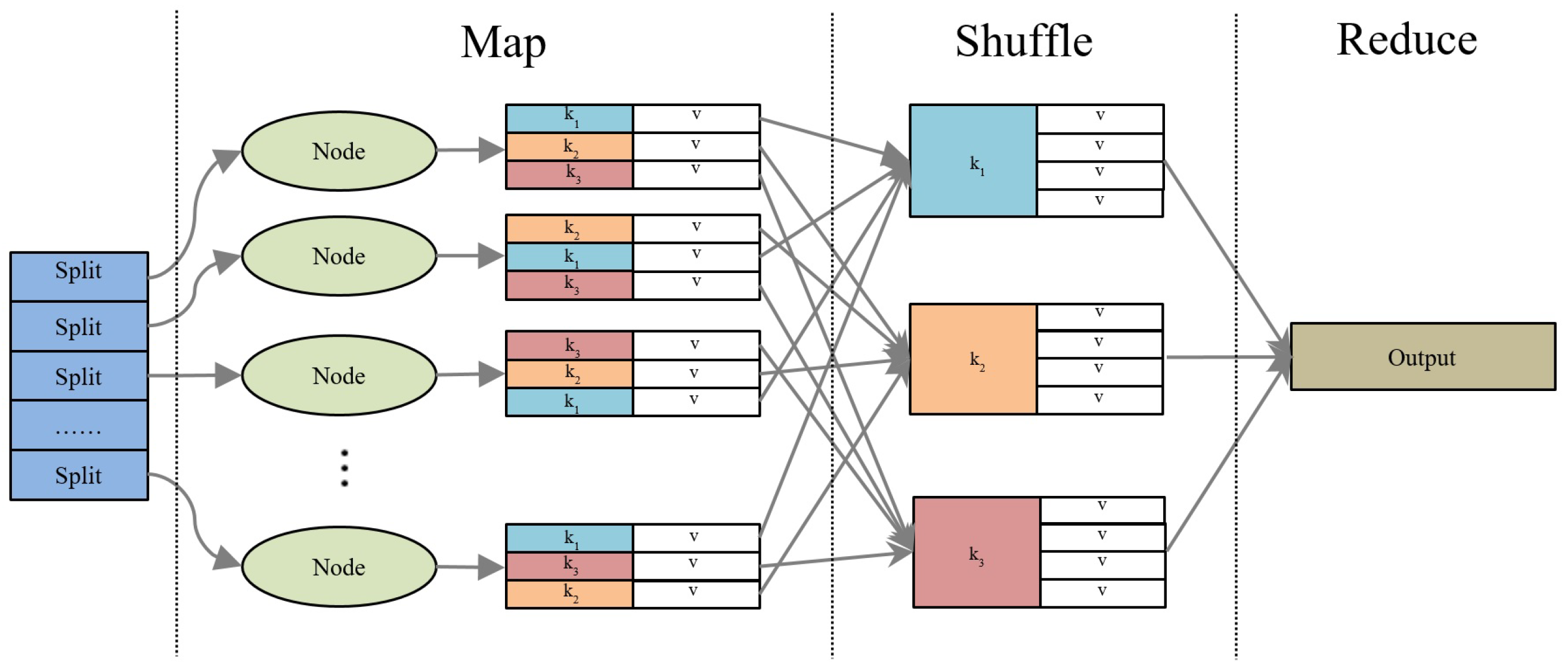
The MapReduce framework is a parallel computing paradigm proposed by Google Inc. It allows large data sets to be tackled over a cluster of computers in a parallel manner regardless of the underlying hardware. It is based on the philosophy that most computing tasks can be performed in the same way and then intermediate results can be aggregated to generate the final results. Such a programming paradigm is implemented based on the Map and Reduce functions, which are inherited from the classical functional programming paradigm. Specifically, the cluster of computers is composed of a master working node and several slave working nodes. In the Map phase, the input data set is divided into independent and disjoint subsets by the master node and then distributed to slave nodes. Then, smaller problems are handled by the slave nodes and then answers for all sub-problems are returned to the master node. Finally, in the Reduce phase, the answers for all sub-problems are combined in some manner to generate the final output by the master node. Thus, in order to utilize the MapReduce framework, one only need to specify what should be calculated in the Map and Reduce functions, while the issue of how to distribute the data among the cluster of working nodes is addressed by the system automatically [52]. It is worty to note that, while alternative frameworks such as Apache Spark offer advantages in iterative tasks and in-memory computation, MapReduce was chosen due to its suitability for handling large-scale data sets with high fault tolerance and low resource requirements. MapReduce’s simplicity and maturity make it an ideal choice for implementing the proposed optimization algorithm in a distributed environment.
Both the Map and Reduce functions employ pairs as input and output. The Map phase takes each pair as input and generates a set of intermediate pairs as output. This could be presented as follows:
Then, the master node merges all the values that share the same intermediate key as a list (known as the shuffle phase). The Reduce phase takes a key and its associated value list as input, and produces the final value. This could be presented as follows:
Figure 2 presents the flowchart of the MapReduce framework.

Figure 2.
Flowchart of the MapReduce framework.
In order to utilize the MapReduce framework to accelerate the computation of and , we need to divide the whole set of pairs of reference alternatives such that into disjoint subsets. Then, each subset is replicated and transfered to working nodes to be handled by a Map task in parallel. A Map task calculates the sum of increments for and based on the subset it receives. Finally, the Reduce task sums over all the outputs generated by each Map task and obtains the final results. In this parallel manner, the MapReduce framework helps to accelerate the computation of and . Algorithms 3 and 4 describe the Map and Reduce phases for calculating , respectively. Since the computation of is similar to that of , we do not present the corresponding algorithm here to save space. Remark that, because and are in additive forms with respect to pairs of reference alternatives such that , the final outcomes are irrelevant for the parallel implementation and this method is robust to the Map and Reduces phases in the MapReduce framework.
| Algorithm 3 Calculate : Map phase. |
Input: where is the index of subset and is the subset of pairs of reference alternatives such that ; the current feasible solution .
Output: . |
| Algorithm 4 Calculate : Reduce phase. |
Input: .
Output: where is equal to . |
With the optimal solution , we can calculate comprehensive values for each alternative . Because the value function constructed with the optimal solution does not guarantee perfect consistency (i.e., reproduction of all assignment examples), we cannot apply the standard example-based value-driven sorting procedure [5] to perform the assignment for alternatives and need a new method to deal with the potential inconsistencies when suggesting assignment. For this purpose, we can calculate the following consistency degree for quantifying the assignment , , and choose with the maximum as the final assignment of alternative a:
This degree indicates a proportion of reference alternatives assigned to a class either worse or better than that attain comprehensive values, respectively, lower or greater than a according to the estimated preference model. Clearly, the greater is, the more justified is the assignment of a to . Hence, we select with the maximal as the recommended category for .
4. Application to University Classification
In this section, we apply the proposed approach to university classification and then examine its performance by analyzing the experimental results. The experimental analysis is based on Best Chinese Universities Rankings (BCUR) in 20183, which provides the overall ranking of 600 universities in China. BCUR ranks universities according to their performances in four dimensions: teaching and learning, research, social service as well as internationalization. The specification of the considered criteria and corresponding indicators in each dimension are summarized in Table 1.

Table 1.
Considered criteria and corresponding indicators in BCUR.
The BCUR 2018 dataset was chosen for several key reasons that make it particularly suitable for validating our proposed method:
- Comprehensive and Multi-Dimensional Ranking: BCUR ranks universities based on their performance in four key dimensions: teaching and learning, research, social service, and internationalization. This multi-dimensional approach aligns well with the nature of multiple criteria sorting (MCS) problems, where decisions are based on multiple criteria.
- Transparency and Reliability: BCUR is known for its transparency, as it not only publishes the detailed methodology and data sources but also provides the raw data of all evaluated indicators. This allows for thorough validation and further analysis, which is crucial for our experimental setup.
- Representativeness: The dataset includes 600 universities from mainland China, providing a broad and representative sample. This ensures that the results obtained from our method are generalizable and can be applied to a wide range of decision-making scenarios.
- Relevance and Practical Application: The ranking criteria used in BCUR are highly relevant to real-world decision-making processes. For example, the “Quality of Incoming Students” indicator reflects the recognition of universities by parents and students, while the “Education Outcome” indicator measures the acceptance of graduates by employers. These criteria are directly applicable to the types of decisions our method aims to support.
- Data Quality and Availability: BCUR provides high-quality, structured data that is publicly available. This makes it an ideal dataset for validating our method, as it ensures the reliability of the results and allows for reproducibility of the experiments.
Although the size of this data set is not large enough, we can compare the performance of the proposed approach to that of the classical UTADIS method for this problem. Since both of the two methods employ an additive value function as the preference model, one can clearly observe the results from them in terms of some measures as well as the shape of the constructed value functions. First, we divide all the 600 universities into five categories according to their total scores. Each category is composed of 120 universities and and are the best and worst categories, respectively. For the convenience of subsequent experimental analysis, the evaluation scale of each criterion is divided into the same number of sub-intervals. In particular, we examine the results for the following numbers of sub-intervals: . The performance of the proposed approach is compared with that of the UTADIS method through cross-validation: the reference set is divided into S (usually ) folds of equal size ensuring that the proportions between categories are the same in each fold as they are in the whole reference set. Then, of the folds are used to train the model that is then evaluated on the remaining fold. This procedure is repeated for all S possible choices, and then the classification accuracies from the S runs are averaged. Since the problem contains only 600 universities, we implement the proposed approach without the MapReduce framework. The UTADIS method and the proposed approach are executed with Java and IBM ILOG CPLEX® solver.
Table 2 reports the average of accuracies for ten-fold cross-validation. It is obvious that the proposed approach has a significant advantage in classification accuracy over the UTADIS method for the same . When , both the proposed approach and the UTADIS method achieve the best performance. Thus, is the optimal setting of the number of sub-intervals on each criterion for this problem. Moreover, the results of the one-tailed paired t-test with the significance level 0.05 to test the statistical significance confirm that the proposed approach performs better than the UTADIS method significantly. The reason underlying the significant difference between the performance of the two methods consists in that the proposed approach not only minimizes the degree of inconsistency when the assignment of violates the consistency principle, but also maximizes the margin to the decision boundary when the assignment of accords the consistency principle, which produces a model that is as both consistent and robust as possible. By contrast, the UTADIS method only focuses on minimizing the sum of inconsistency degrees between the comprehensive values of reference alternatives and the respective category thresholds. When the assignment examples of reference alternatives are consistent (e.g., the considered problem of university classification), there are multiple optimal solutions for the UTADIS method. In this case, the selected value function selected by the UTADIS method is very likely to be different from the true one.
Table 2.
Accuracy of different methods for the problem of university classification.
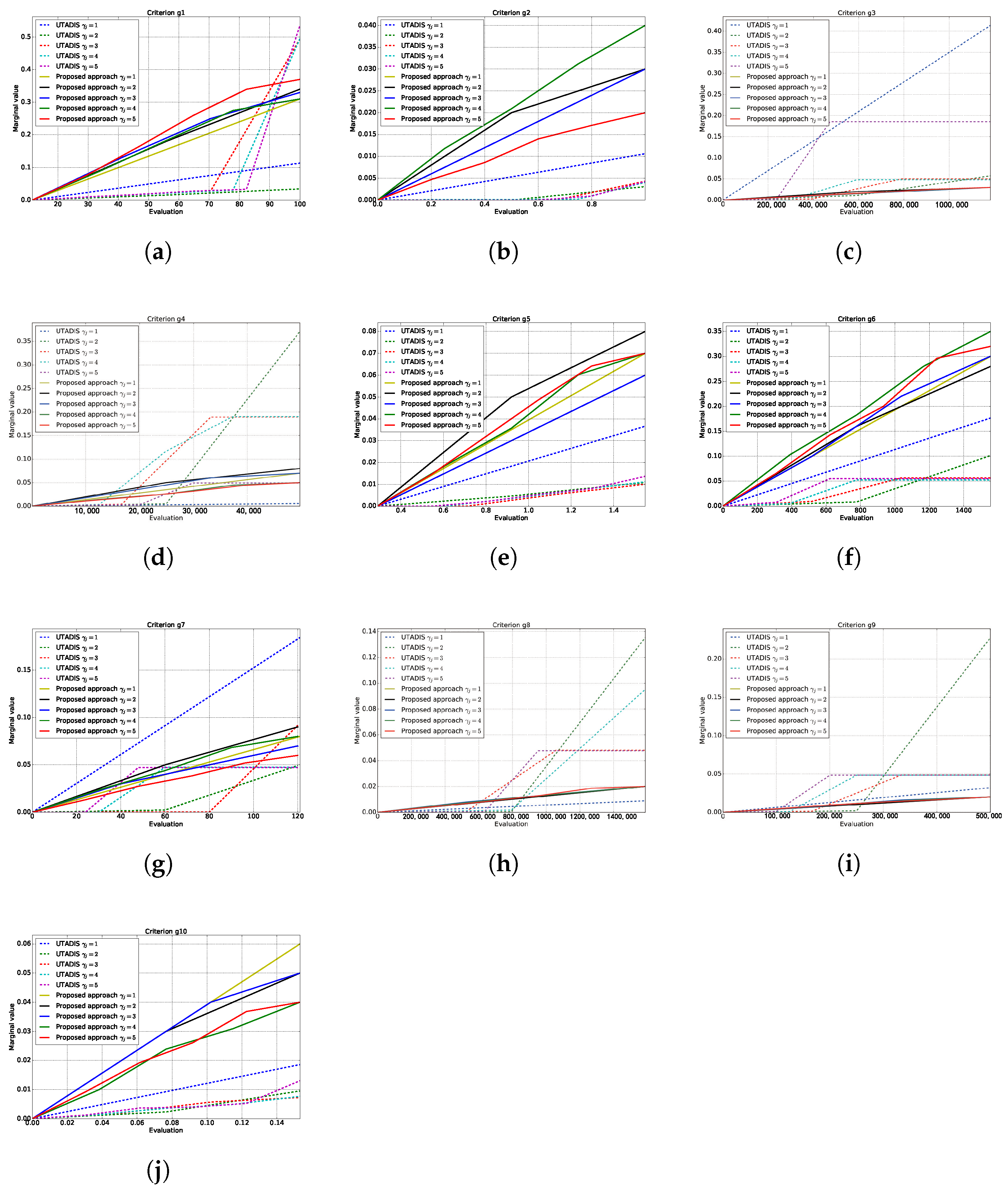
Then, we use the whole reference set as the training data to derive value functions using different methods and depict marginal value functions on each criterion in Figure 3. The trade-off weights of criteria derived from different methods are reported in Table 3. We observe that the shape of marginal value functions derived from the UTADIS method with different differ from each other significantly. Moreover, the trade-off weights for the same criterion with different vary significantly. This indicates that the UTADIS method is not robust to the way of dividing the range of evaluation into sub-intervals, which makes the trade-off weights for criteria unstable and the results difficult to interpret. In contrast to the UTADIS method, the marginal value functions derived from the proposed approach are more smooth than those generated by UTADIS method. Additionally, the trade-off weights for the same criterion with different do not vary significantly. Thus, the proposed approach seems to be robust to the way of dividing the range of evaluation into sub-intervals.
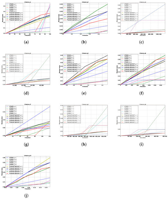
Figure 3.
Marginal value functions derived from UTADIS and the proposed approach. (a) -Quality of incoming students. (b) -Education outcome. (c) -Reputation. (d) -Scale of research. (e) -Quality of research. (f) -Top research achievements. (g) -Top scholars. (h) -Technology service. (i) -Technology transfer. (j) -International student ratio.
Table 3.
Trade-off weights of criteria derived from different methods.
5. Simulation Experiments
This section presents the experimental analysis that was performed to examine the performance of the proposed approach in dealing with large-scale MCS problems. First, Section 5.1 describes the performance measures used to evaluate the proposed approach. Section 5.2 presents the configuration details for the hardware and software used in our experiments. Section 5.3 describes the generation of the data, the factors considered in the implementation, and the general experimental process. Section 5.4 reports and discusses the obtained results.
5.1. Performance Measures
In this work, we study the implementation of the MapReduce framework for the proposed approach. Thus, we can evaluate the performance of the proposed approach according to the following measures.
- Accuracy: This measure quantifies how many alternatives are correctly classified by the proposed approach. In our experiments, we only focus on the classification accuracy on the set of non-reference alternatives A.
- Runtime: This metric quantifies the overall computational time required by the proposed approach.
- Speedup: This measure compares the efficiency of the proposed approach implemented with a parallel system to that achieved by the sequential version on a single node. It can be calculated as
5.2. Hardware and Software
The MapReduce framework in this study is implemented on seven working nodes in a cluster: one master node and six working nodes. All the working nodes share the same configurations as follows:
- Processors: 2 × Intel Xeon E5-2620.
- Cores: 6 per processor (12 threads).
- Clock speed: 2 GHz.
- Cache: 15 MB.
- Network connection: Intel 82579LM Gigabit.
- Hard drive: 1 TB (7200 rps).
- RAM: 32 GB.
The software for implementing the MapReduce framework and associated settings are as follows:
- Operating system: Ubuntu 14.04 Server.
- MapReduce implementation: Hadoop 2.6.0.
- Maximum map tasks: 128.
- Maximum reduce task: 1.
5.3. Experimental Design
The investigation is based on the generation of random data that follows a uniform distribution. We describe the relevant factors in the simulation in Table 4:
Table 4.
Factors investigated in the experimental design.
We adopt a ceteris paribus design in the following experimental analysis and begin the experiments from the benchmark of the problem setting as follows: K, , , and . Then, we consider different levels of one factor while keeping others fixed to investigate its impact on the results. For each problem setting, 50 data sets are randomly generated to test the performance of the proposed approach. Each data set is equally divided into two subsets: the reference set and the test set A. The reference set is used to develop the sorting model, and the test set A is used to test the performance of the proposed approach. Both the two sets contain the same number of alternatives.
In the phase of data generation in each experiment, we first specify the actual value function and the actual category thresholds. Then, the actual assignment of alternatives can be determined by calculating their comprehensive values and comparing them to category thresholds. We specify the actual preference model in a way such that the number of alternatives is equally distributed in all the categories for both and A. Note that for each generated data set, we mislabel the assignment of 5% of the reference alternatives in , considering them to be inconsistent assignment examples.
The general experimental process is described as follows:
Select a specific problem setting. For the problem involving alternatives and m criteria, drawing values randomly from a uniform distribution [0, 1] to generate an evaluation matrix.
Specify the actual preference model, including the actual value function and the actual category thresholds.
Obtain actual assignment outcomes for alternatives in and A by calculating their comprehensive values and comparing them to category thresholds.
Apply the proposed approach to develop a preference model.
Determine the assignment outcomes by applying the developed preference model to the set of alternatives .
Compare the two assignment outcomes, and evaluate the performance of the proposed approach by collecting the accuracy, runtime, and speedup.
5.4. Experimental Results
This section describes and analyzes the results generated in the experimental study. The performance of the proposed approach is evaluated in terms of the accuracy, runtime, and speedup. In the following, we present the results and analysis for various levels of the considered factors.
5.4.1. Performance Evaluation on Different Numbers of Alternatives
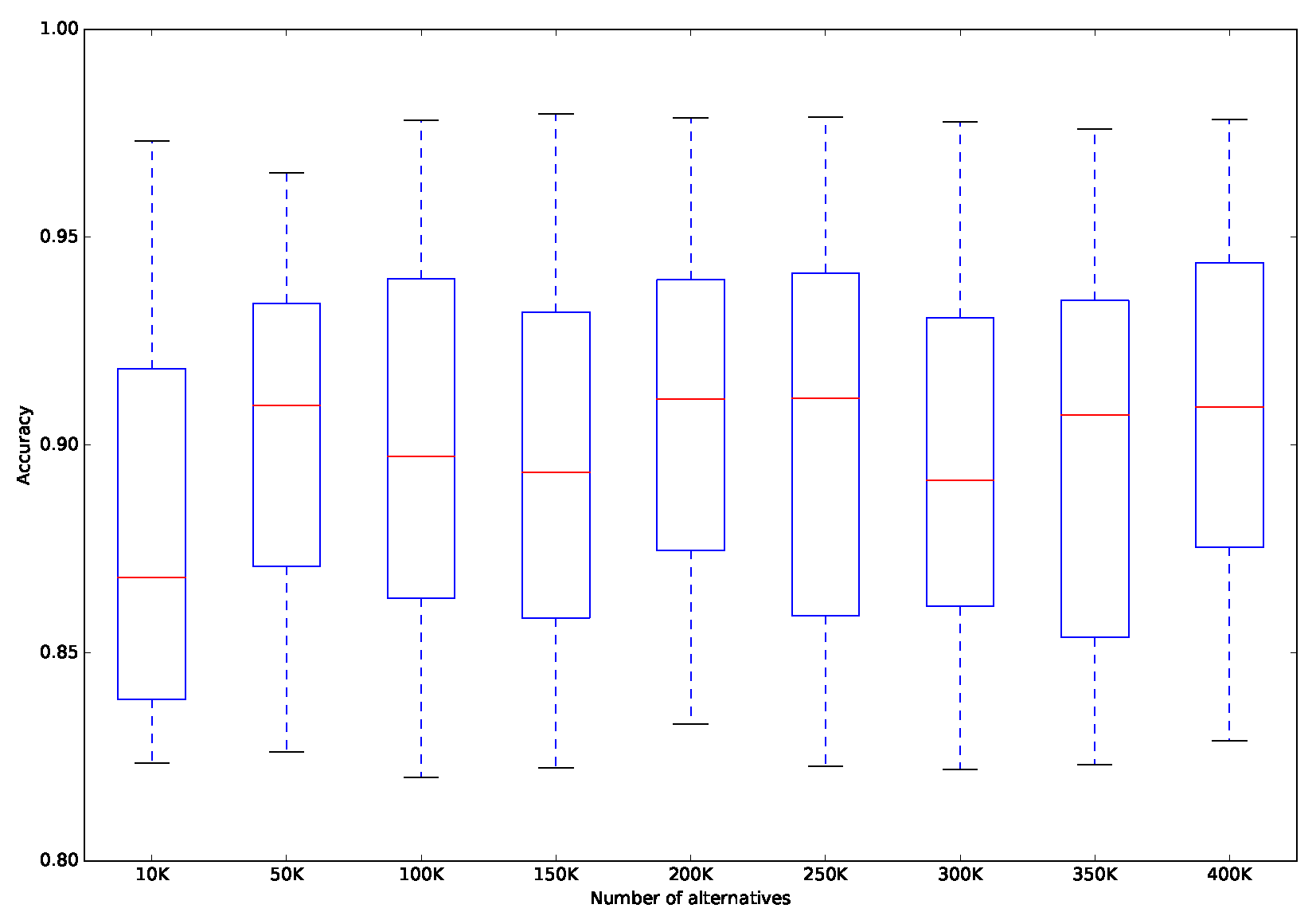
Table 5 and Figure 4 summarize the results obtained on the generated data sets with different numbers of alternatives. Other than the number of alternatives, the other settings remain the same as the benchmark. Table 5 presents the minimum, maximum, average, and standard deviation of the accuracy and the average of the computational time. Figure 4 plots the “Box and Whisker” graph, to show the distribution of the accuracy for different numbers of alternatives. From Table 5, we observe that there is no noticeable tendency in the variation of the classification accuracy when the number of alternatives varies. This is because we use the same method for generating the experimental data sets, and thus all of the generated data sets share a similar problem structure, although they have different numbers of alternatives. On the other hand, we observe from Table 5 that a longer runtime is required for the proposed approach as the number of alternatives increases. This is because that more alternatives bring more pairwise comparisons between reference alternatives and the proposed approach needs more runtime to handle large-scale reference sets. However, note that traditional MCS methods cannot deal with such large-scale problems because it exceeds processing capabilities of these methods in terms of memory consumption and computational time. By contrast, the proposed approach provides a feasible way of handling huge amounts of data.
Table 5.
Results obtained for different numbers of alternatives.

Figure 4.
Distribution of accuracy for different numbers of alternatives.
5.4.2. Performance Evaluation on Different Numbers of Criteria
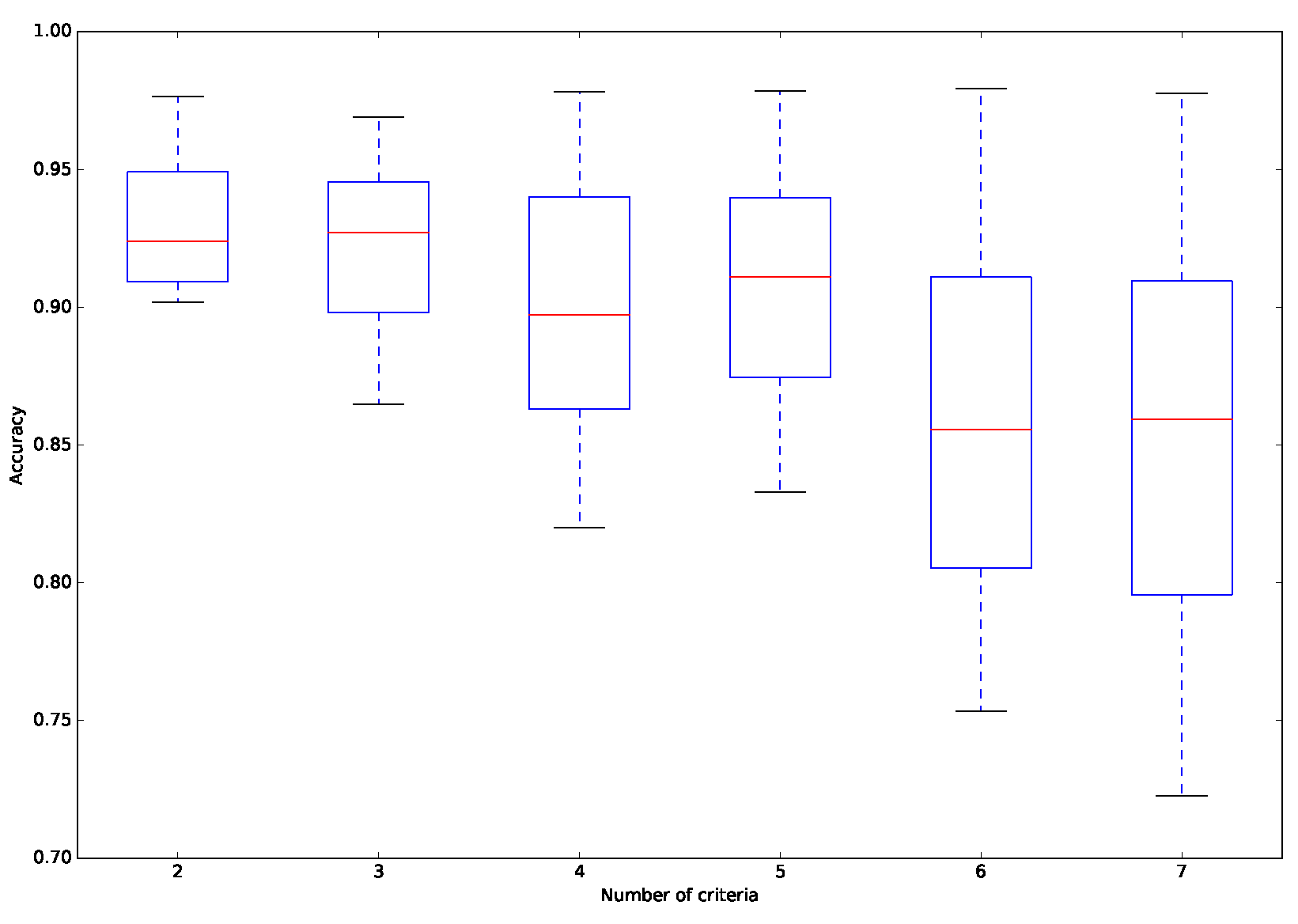
In this part, we focus on the analysis of the performance of the approach on data sets with different numbers of criteria. Table 6 and Figure 5 present the obtained results. As we can see, the accuracy gradually decreases and its standard deviation increases as the number of criteria increases. Specifically, the proposed approach can achieve an average of accuracy of 0.930 when the number of criteria is only two. The average of accuracy drops below 0.860 when the number of criteria reaches seven. The reason for this is that when there are more criteria, the preference model contains more parameters that need to be estimated, and thus it becomes more difficult for the proposed approach to infer a preference model sufficiently close to the actual one, which increases the number of incorrect assignment. On the other hand, it can be observed from Table 6 that although the difficulty of solving the problem increases when dealing with more criteria, the computational time of the proposed approach does not increase dramatically, ranging from 952.251 s for two criteria to 1271.060 s for seven criteria.
Table 6.
Results obtained for different numbers of criteria.
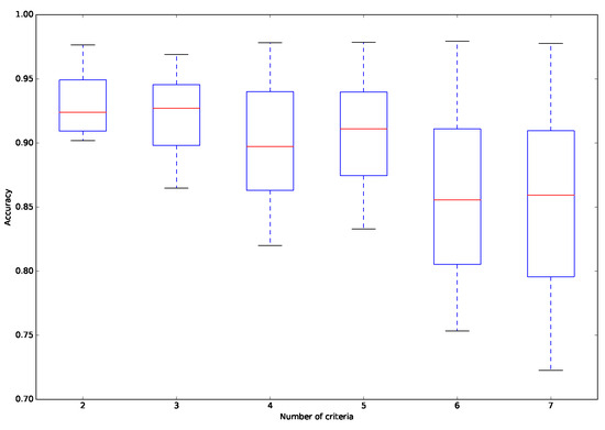
Figure 5.
Distribution of accuracy for different numbers of criteria.
To analyze this phenomenon further, we measure the difference between the inferred preference model and the actual one by calculating the Euclidean distance between the two models’ weight vectors. The outcomes are summarized in Table 7, showing that when there are more criteria, the Euclidean distance between the two models’ weight vectors becomes larger. Thus, the ability of the proposed approach to infer a weight vector that is close to the actual one deteriorates when dealing with more criteria, which is the main reason for the occurrence of more incorrect assignment. However, this argument assumes that the considered criteria are not correlated. When the criteria are highly correlated, the inferred preference model will barely change from the actual one.
Table 7.
Results obtained for different numbers of criteria.
5.4.3. Performance Evaluation on Different Numbers of Categories
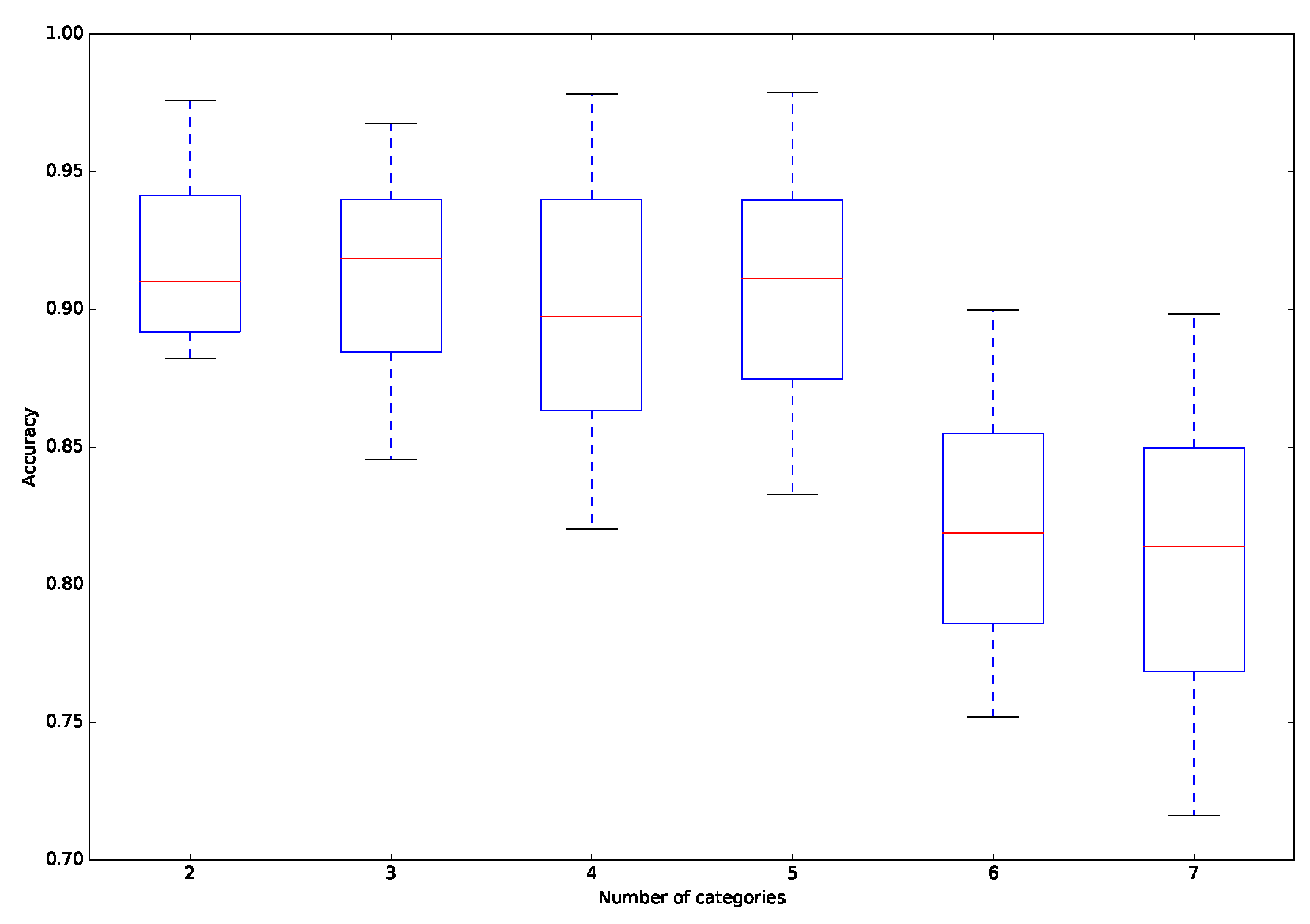
This section focuses on the study of the performance of the approach in dealing with different numbers of categories. As Table 8 and Figure 6 clearly show, the average of the accuracy decreases and the variation of the accuracy increases when there are more categories. More precisely, the average of the accuracy decreases from 0.917 to 0.810, while the variation in the accuracy increases from 0.030 to 0.053. This reveals that the difference between the inferred preference model and the actual model increases when dealing with more categories, because the presence of more categories introduces more flexibility to the considered problem. On the other hand, the runtime of the proposed approach increases when dealing with more categories, because more pairwise comparisons between reference alternatives must be considered in the phase of inferring the parameters of the preference model.
Table 8.
Results obtained for different numbers of categories.
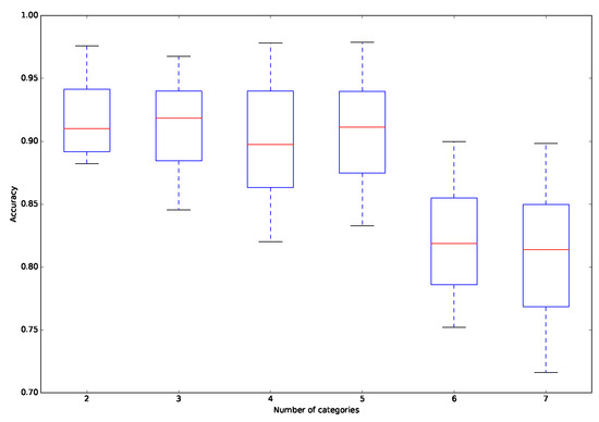
Figure 6.
Distribution of accuracy for different numbers of categories.
In addition, we count the number of incorrect assignment for various differences between the predicted assignment and the actual one. The difference between the predicted assignment and the actual one is defined as the absolute difference between the indices of the two assignment. For example, if the actual assignment for an alternative is category but it is assigned to category by the proposed approach, then the difference between the predicted assignment and the actual one for the alternative a is two. Table 9 summarizes the percentage of incorrect assignment with various differences between the predicted assignment and the actual one in cases of different numbers of categories. One can observe that the difference between most wrong assignment and the corresponding actual assignment is one, even in the case of six or seven categories. This indicates that although the performance of the proposed approach deteriorates as the number of categories increases, alternatives that are misclassified are assigned to categories that are close to their actual assignment, and such outcomes can be accepted by the DM.
Table 9.
Results obtained for different numbers of categories.
5.4.4. Performance Evaluation on Different Numbers of Working Nodes
In this section, we aim to study the influence of the number of working nodes on the performance of the proposed approach. Table 10 presents the average runtime and the speedup achieved by the proposed approach. Note that we perform all comparisons on the same data sets in this section. Given the results, we wish to make the following comments. On the one hand, because we utilize the MapReduce framework to accelerate the computation of the coefficients for the LP model and work out recommended assignment for non-reference alternatives, the achieved accuracy of the final outcomes is independent of the number of working nodes used in the implementation. On the other hand, as the computational complexity remains the same for each certain problem, more working nodes will accelerate the computational process and improve the efficiency of the approach. Thus, one can observe that the runtime decreases and the speedup increases as the number of working nodes increases.
Table 10.
Results obtained for different numbers of working nodes.
Table 11 and Figure 7 report the runtime for different numbers of alternatives and working nodes. We can observe that the runtime under different settings varies significantly: when six working nodes are used to deal with 10 K alternatives, less than one minute is needed to solve the problem; when addressing 400 K alternatives with only one working node, the proposed approach spend more than 10,000 s. On the other hand, although more alternatives induce more pairwise comparisons, of which the complexity is , the runtime does not increase in a ratio of . This is due to the characteristics of the Hadoop platform, such as the load balance technique, which enhances the performance of the proposed approach and improves the computation efficiency during the process.
Table 11.
Runtime for different numbers of alternatives and working nodes.
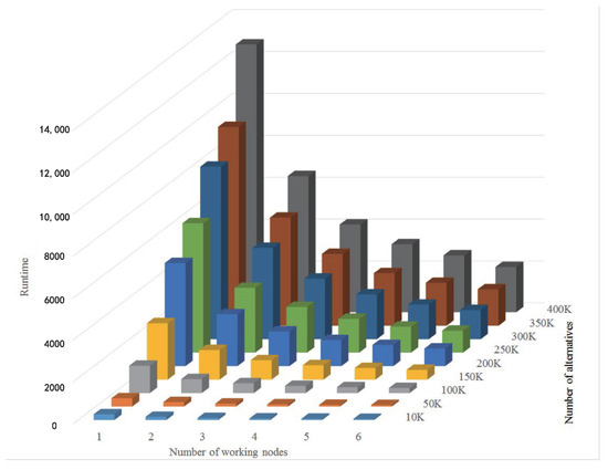
Figure 7.
Runtime for different numbers of alternatives and working nodes.
6. Conclusions
In this paper, we develop a new MCS approach based on the MapReduce framework for dealing with a large set of alternatives and massive preference information. This approach utilizes the preference disaggregation paradigm to construct a convex optimization model, which aims to infer a preference model in form of a piecewise-linear additive value function from assignment examples on reference alternatives. Such an model considers the consistency and robustness concerns of the preference model simultaneously and avoids using slack variables to specify the degrees of inconsistency for assignment examples, which is especially suitable for addressing large-scale MCS problems. Then, a new parallel algorithm is developed to solve this optimization model and the MapReduce framework is utilized to deal with the set of reference alternatives and associated preference information in a parallel manner in order to accelerate the computation.
The main advantage of the proposed approach consists in its scalability in dealing with large sets of alternatives and massive preference information. It avoids using slack variables to construct a preference model and thus contains a relatively small set of variables and linear constraints. Then, it utilizes the MapReduce framework to deal with the set of reference alternatives and associated preference information in a parallel manner, and has no specific requirements on the processing capabilities on working nodes. Moreover, the proposed approach is robust to the parallel implementation, and the final outcomes are irrelevant to the splitting and the combining operations in the MapReduce framework. Therefore, it is not necessary to specify particular operations for how to split the original data set and aggregate the intermediate results.
We acknowledge that our approach relies on an additive piecewise-linear value function, which assumes preferential independence among criteria. While this assumption simplifies the model and enhances computational efficiency, it may not adequately capture complex, non-linear preference structures that are common in real-world decision-making scenarios. Non-linear preference structures can arise when the interaction effects between criteria significantly influence the overall preference. For example, in certain multi-criteria optimization problems, the combined effect of two criteria may be greater than the sum of their individual effects. Our method, as currently formulated, does not account for such interactions, which could lead to suboptimal decision outcomes in scenarios where non-linear preferences are prevalent. Moreover, the performance of our approach is inherently dependent on the quality of the input data. Inaccurate or noisy data can lead to misleading preference models and, consequently, incorrect decision recommendations. For instance, if the assignment examples provided by the decision maker are inconsistent or contain errors, the inferred value function may not accurately reflect the true preferences. This sensitivity is a common challenge in data-driven decision-making and underscores the importance of robust data preprocessing and validation steps. While our method includes mechanisms to handle some degree of inconsistency in the data, it is not immune to the detrimental effects of poor data quality.
We consider the extension of this approach in several interesting directions. First, a real-world application for a large-scale MCS problem is required to validate the proposed approach. Second, in cases where significant interactions are expected, future extensions of our work could incorporate more sophisticated preference models that account for such interactions, such as non-additive value functions or models that explicitly consider criterion interdependencies. Third, another interesting direction would be to employ other types of preference models, such as outranking preference models and rule induction model, to address the considered MCS problem with the MapReduce framework. This needs developing hybrid models that combine the strengths of outranking, rule-based, and value function approaches. Such models could offer greater flexibility and robustness in handling diverse decision scenarios. Moreover, it requires exploring how to further enhance the scalability of outranking and rule-based models when applied to large-scale datasets. This could involve optimizing the computational efficiency of these models or developing novel parallelization strategies.Finally, by incorporating multiple datasets and rigorous validation techniques in future research, we aim to strengthen the external validity and generalizability of our findings. This will ensure that our method is not only scalable but also reliable and applicable across a wide range of decision-making scenarios.
Author Contributions
Conceptualization, X.M.; methodology, X.M.; software, L.Z.; validation, L.Z.; investigation, Z.D.; resources, Z.D.; data curation, Z.D.; writing—original draft preparation, X.M.; writing—review and editing, L.Z.; visualization, L.Z.; project administration, Z.D. All authors have read and agreed to the published version of the manuscript.
Funding
This research was funded by the National Natural Science Foundation of China (Grant No. 72401227), Humanities and Social Science Fund of Ministry of Education of China (Grant No. 24XJC630007, Grant No. 24XJC630022).
Data Availability Statement
The data that support the findings of this study are available from the corresponding author upon reasonable request.
Conflicts of Interest
The authors declare no conflicts of interest.
Notes
| 1 | Available online: http://www-01.ibm.com/software/data/bigdata/what-is-big-data.html (accessed on 18 November 2024). |
| 2 | Available online: http://www.investopedia.com/articles/active-trading/040915/how-big-data-has-changed-finance.asp (accessed on 24 October 2021). |
| 3 | Available online: http://www.shanghairanking.com/Chinese_Universities_Rankings/Overall-Ranking-2018.html (accessed on 16 March 2018). |
References
- Şenel, G. An Innovative Algorithm Based on Octahedron Sets via Multi-Criteria Decision Making. Symmetry 2024, 16, 1107. [Google Scholar] [CrossRef]
- Topal, A.; Bayazit, N.G.; Ucan, Y. A Method to Handle the Missing Values in Multi-Criteria Sorting Problems Based on Dominance Rough Sets. Mathematics 2024, 12, 2944. [Google Scholar] [CrossRef]
- Qin, J.; Liang, Y.; Luis, M.; Ishizaka, A.; Pedrycz, W. ORESTE-SORT: A novel multiple criteria sorting method for sorting port group competitiveness. Ann. Oper. Res. 2023, 325, 875–909. [Google Scholar] [CrossRef]
- Roy, B. Multicriteria Methodology for Decision Aiding; Springer US: Berlin/Heidelberg, Germany, 1996. [Google Scholar]
- Greco, S.; Mousseau, V.; Słowiński, R. Multiple criteria sorting with a set of additive value functions. Eur. J. Oper. Res. 2010, 207, 1455–1470. [Google Scholar] [CrossRef]
- Kadziński, M.; Wójcik, M.; Ciomek, K. Review and experimental comparison of ranking and choice procedures for constructing aunivocal recommendation in a preference disaggregation setting. Omega 2022, 113, 102715. [Google Scholar] [CrossRef]
- Greco, S.; Słowiński, R.; Wallenius, J. Fifty years of multiple criteria decision analysis: From classical methods to robust ordinal regression. Eur. J. Oper. Res. 2024, 323, 351–377. [Google Scholar] [CrossRef]
- Chi, S.Y.; Chien, L.H. Why defuzzification matters: An empirical study of fresh fruit supply chain management. Eur. J. Oper. Res. 2023, 311, 648–659. [Google Scholar] [CrossRef]
- Barbati, M.; Greco, S.; Lami, I.M. The Deck-of-cards-based Ordinal Regression method and its application for the development of an ecovillage. Eur. J. Oper. Res. 2024, 319, 845–861. [Google Scholar] [CrossRef]
- Torkayesh, A.E.; Hendiani, S.; Walther, G.; Venghaus, S. Fueling the future: Overcoming the barriers to market development of renewable fuels in Germany using a novel analytical approach. Eur. J. Oper. Res. 2024, 316, 1012–1033. [Google Scholar] [CrossRef]
- Camanho, A.S.; Stumbriene, D.; Barbosa, F.; Jakaitiene, A. The assessment of performance trends and convergence in education and training systems of European countries. Eur. J. Oper. Res. 2023, 305, 356–372. [Google Scholar] [CrossRef]
- Mao, X. Scalable preference disaggregation: A multiple criteria sorting approach based on the MapReduce framework. In Proceedings of the Da2pl: From Multiple Criteria Decision Aid to Preference Learning, Poznań, Poland, 22–23 November 2018. [Google Scholar]
- Doumpos, M.; Zopounidis, C. Disaggregation analysis and statistical learning: An integrated framework for multicriteria decision support. In Handbook of Multicriteria Analysis; Springer: Berlin/Heidelberg, Germany, 2010; pp. 215–240. [Google Scholar]
- Corrente, S.; Greco, S.; Kadziński, M.; Słowiński, R. Robust ordinal regression in preference learning and ranking. Mach. Learn. 2013, 93, 381–422. [Google Scholar] [CrossRef]
- Marinakis, Y.; Marinaki, M.; Doumpos, M.; Matsatsinis, N.; Zopounidis, C. Optimization of nearest neighbor classifiers via metaheuristic algorithms for credit risk assessment. J. Glob. Optim. 2008, 42, 279–293. [Google Scholar] [CrossRef]
- Angilella, S.; Mazzù, S. The financing of innovative SMEs: A multicriteria credit rating model. Eur. J. Oper. Res. 2015, 244, 540–554. [Google Scholar] [CrossRef]
- Doumpos, M.; Figueira, J.R. A multicriteria outranking approach for modeling corporate credit ratings: An application of the Electre Tri-nC method. Omega 2019, 82, 166–180. [Google Scholar] [CrossRef]
- Liou, J.J.; Tzeng, G.H. A dominance-based rough set approach to customer behavior in the airline market. Inf. Sci. 2010, 180, 2230–2238. [Google Scholar] [CrossRef]
- Liu, J.; Liao, X.; Huang, W.; Liao, X. Market segmentation: A multiple criteria approach combining preference analysis and segmentation decision. Omega 2019, 83, 1–13. [Google Scholar] [CrossRef]
- Doumpos, M.; Zopounidis, C. Computational intelligence techniques for multicriteria decision aiding: An overview. In Multicriteria Decision Aid and Artificial Intelligence; Wiley: Hoboken, NJ, USA, 2013; pp. 1–23. [Google Scholar]
- Nocedal, J.; Wright, S.J. Numerical Optimization; Springer: Berlin/Heidelberg, Germany, 2004. [Google Scholar]
- Bardis, G. A Declarative Modeling Framework for Intuitive Multiple Criteria Decision Analysis in a Visual Semantic Urban Planning Environment. Electronics 2024, 13, 4845. [Google Scholar] [CrossRef]
- Wen, Z.; Liao, H.; Shi, Y. PL-MACONT-I: A Probabilistic Linguistic MACONT-I Method for Multi-Criterion Sorting. Int. J. Inf. Technol. Decis. Mak. 2024, 23, 269–288. [Google Scholar] [CrossRef]
- Doumpos, M.; Zopounidis, C. Multicriteria Decision Aid Classification Methods; Springer Science & Business Media: Berlin/Heidelberg, Germany, 2002. [Google Scholar]
- Köksalan, M.; Özpeynirci, S.B. An interactive sorting method for additive utility functions. Comput. Oper. Res. 2009, 36, 2565–2572. [Google Scholar] [CrossRef]
- Liu, J.; Kadzinski, M.; Liao, X. Modeling Contingent Decision Behavior: A Bayesian Nonparametric Preference-Learning Approach. Informs J. Comput. 2023, 35, 764–785. [Google Scholar] [CrossRef]
- Liu, J.; Kadzinski, M.; Liao, X.; Mao, X. Data-Driven Preference Learning Methods for Value-Driven Multiple Criteria Sorting with Interacting Criteria. Informs J. Comput. 2021, 35, 419–835. [Google Scholar] [CrossRef]
- Ru, Z.; Liu, J.; Kadziński, M.; Liao, X. Probabilistic ordinal regression methods for multiple criteria sorting admitting certain and uncertain preferences. Eur. J. Oper. Res. 2023, 311, 596–616. [Google Scholar] [CrossRef]
- Yu, W. ELECTRE TRI: Aspects méthodologiques et manuel d’utilisation. In Document-Université de Paris-Dauphine; LAMSADE: Paris, France, 1992. [Google Scholar]
- Cailloux, O.; Meyer, P.; Mousseau, V. Eliciting ELECTRE TRI category limits for a group of decision makers. Eur. J. Oper. Res. 2012, 223, 133–140. [Google Scholar] [CrossRef]
- Zheng, J.; Takougang, S.A.M.; Mousseau, V.; Pirlot, M. Learning criteria weights of an optimistic Electre Tri sorting rule. Comput. Oper. Res. 2014, 49, 28–40. [Google Scholar] [CrossRef]
- Fernández, E.; Figueira, J.R.; Navarro, J.; Roy, B. ELECTRE TRI-nB: A new multiple criteria ordinal classification method. Eur. J. Oper. Res. 2017, 263, 214–224. [Google Scholar] [CrossRef]
- Almeida-Dias, J.; Figueira, J.R.; Roy, B. Electre Tri-C: A multiple criteria sorting method based on characteristic reference actions. Eur. J. Oper. Res. 2010, 204, 565–580. [Google Scholar] [CrossRef]
- Almeida-Dias, J.; Figueira, J.R.; Roy, B. A multiple criteria sorting method where each category is characterized by several reference actions: The Electre Tri-nC method. Eur. J. Oper. Res. 2012, 217, 567–579. [Google Scholar] [CrossRef]
- Köksalan, M.; Mousseau, V.; Özpeynirci, Ö.; Özpeynirci, S.B. A new outranking-based approach for assigning alternatives to ordered classes. Nav. Res. Logist. 2009, 56, 74–85. [Google Scholar] [CrossRef]
- Kadziński, M.; Ciomek, K. Integrated framework for preference modeling and robustness analysis for outranking-based multiple criteria sorting with ELECTRE and PROMETHEE. Inf. Sci. 2016, 352, 167–187. [Google Scholar] [CrossRef]
- Nemery, P.; Lamboray, C. Flowsort: A flow-based sorting method with limiting or central profiles. Top 2008, 16, 90–113. [Google Scholar] [CrossRef]
- Greco, S.; Matarazzo, B.; Slowinski, R. Rough sets theory for multicriteria decision analysis. Eur. J. Oper. Res. 2001, 129, 1–47. [Google Scholar] [CrossRef]
- Kadziński, M.; Greco, S.; Słowiński, R. Robust ordinal regression for dominance-based rough set approach to multiple criteria sorting. Inf. Sci. 2014, 283, 211–228. [Google Scholar] [CrossRef]
- Devaud, J.; Groussaud, G.; Jacquet-Lagreze, E. UTADIS: Une méthode de Construction de Fonctions d’utilité Additives Rendant Compte de Jugements Globaux; European Working Group on Multicriteria Decision Aid: Bochum, Germany, 1980; p. 94. [Google Scholar]
- Greco, S.; Kadziński, M.; Mousseau, V.; Słowiński, R. Robust ordinal regression for multiple criteria group decision: UTA GMS-GROUP and UTADIS GMS-GROUP. Decis. Support Syst. 2012, 52, 549–561. [Google Scholar] [CrossRef]
- Corrente, S.; Doumpos, M.; Greco, S.; Słowiński, R.; Zopounidis, C. Multiple criteria hierarchy process for sorting problems based on ordinal regression with additive value functions. Ann. Oper. Res. 2017, 251, 117–139. [Google Scholar] [CrossRef]
- Mousseau, V.; Słowiński, R. Inferring an ELECTRE TRI model from assignment examples. J. Glob. Optim. 1998, 12, 157–174. [Google Scholar] [CrossRef]
- Dias, L.C.; Clímaco, J.N. On computing ELECTRE’s credibility indices under partial information. J. Multi-Criteria Decis. Anal. 1999, 8, 74–92. [Google Scholar] [CrossRef]
- Dias, L.; Mousseau, V.; Figueira, J.; Clímaco, J. An aggregation/disaggregation approach to obtain robust conclusions with ELECTRE TRI. Eur. J. Oper. Res. 2002, 138, 332–348. [Google Scholar] [CrossRef]
- Doumpos, M.; Marinakis, Y.; Marinaki, M.; Zopounidis, C. An evolutionary approach to construction of outranking models for multicriteria classification: The case of the ELECTRE TRI method. Eur. J. Oper. Res. 2009, 199, 496–505. [Google Scholar] [CrossRef]
- Kadziński, M.; Tervonen, T.; Figueira, J.R. Robust multi-criteria sorting with the outranking preference model and characteristic profiles. Omega 2015, 55, 126–140. [Google Scholar] [CrossRef]
- Greco, S.; Figueira, J.; Ehrgott, M. Multiple Criteria Decision Analysis. Springer: Berlin/Heidelberg, Germany, 2016; Volume 37. [Google Scholar]
- Liu, J.; Liao, X.; Huang, W.; Yang, J.b. A new decision-making approach for multiple criteria sorting with an imbalanced set of assignment examples. Eur. J. Oper. Res. 2018, 265, 598–620. [Google Scholar] [CrossRef]
- Murphy, K.P. Machine Learning: A Probabilistic Perspective; MIT Press: Cambridge, MA, USA, 2012. [Google Scholar]
- Bertsimas, D.; Tsitsiklis, J.N. Introduction to linear optimization; Athena Scientific: Belmont, MA, USA, 1997; Volume 6. [Google Scholar]
- Del Río, S.; López, V.; Benítez, J.M.; Herrera, F. On the use of MapReduce for imbalanced big data using random forest. Inf. Sci. 2014, 285, 112–137. [Google Scholar] [CrossRef]

Disclaimer/Publisher’s Note: The statements, opinions and data contained in all publications are solely those of the individual author(s) and contributor(s) and not of MDPI and/or the editor(s). MDPI and/or the editor(s) disclaim responsibility for any injury to people or property resulting from any ideas, methods, instructions or products referred to in the content. |
© 2025 by the authors. Licensee MDPI, Basel, Switzerland. This article is an open access article distributed under the terms and conditions of the Creative Commons Attribution (CC BY) license (https://creativecommons.org/licenses/by/4.0/).