Bounding the Solution Space of Complex Systems in Terms of Non-Numeric and\or Uncontrollable Scenario Variables

Abstract

This paper describes an approach to blend several qualitative and quantitative methods to establish the boundaries of complex systems in terms of uncontrollable, non-numeric variables. Decision makers increasingly encounter layered, multidimensional, interconnected issues that contain unknown unknowns, vast uncertainties, and ill-defined lines of demarcation between the beginning and the end of the problem. The inexactness of boundaries in a systems problem is a result of not knowing important variables, existence of uncontrollable variables, and near-uncountable significant interactions among the variables. Furthermore, complexities and systems challenges arise from unexpected emergent behavior(s) that are often the primary concerns of systems engineers. The ability to investigate uncontrollable variables and their interactions with the system of interest is a critical step for bounding the system problem and defining the solution space. Thus, this paper focuses on developing a means for systematically examining these variables. By incorporating scenario-based computer simulations, scenario discretization, and customized designs of experiments, the authors offer systems engineers and scientists an approach for defining a viable solution space of a complex problem by developing constraint equations from uncontrollable, non-numeric variables.

1. Introduction

1.1. Challenges for Bounding the Engineering Problem

In systems engineering, optimization, or other closely related fields, bounding the system of interest or problem is the first step for defining and understanding the solution space. If the boundary is unknown, then the system is insufficiently defined, thereby constituting an ill-defined engineering problem. Consequently, resultant solutions are either incorrect, illogical, possibly contain unintended consequences, or suffer from some or all these traits [1]. To bound a system or problem means to understand the limitations, objectives, variables, and important quantities that are relevant to the problem and potential solution(s). While these necessary conditions for solving a system problem are readily apparent, inadequate problem definition is a common reason for failure in engineered or complex systems [2] and leads to ineffective or negligible system solutions [3].

Characteristics of systems engineering problems reside in three engineering elements: specifications, variables, and knowledge about the problem [4]. The most difficult of these elements are variables that the engineer does not or cannot control. Therefore, efforts to understand how uncontrollable variables may affect the system solution is a primary concern and an area of continued study. This paper offers a method to establish boundaries of a systems problem in terms of uncontrollable variables. This approach can aid practitioners define the solution space and derive credible solutions.

1.2. An Overview of System Boundaries and Constraints

A boundary separates a system of interest from the environment [5]. The system of interest is the complete entity which is the focus of the problem [6]. However, operational factors that directly influence or interact with the system must also be considered. We further specify that the system of interest is complex as defined by its multidisciplinary nature and non-linearity as the result of emergent behaviors from many interactions among components or system variables [6]. The system boundary defines what features belong to the system, as well as variables that must be in the calculus for developing a system solution. All else is the environment as depicted in Figure 1. Once drawn, the boundary outlines the system of interest and its area of concern, scopes the problem, establishes interface conditions, and most importantly, highlights the solutions space [7]. This final concept for the system of interest and the surrounding boundary are where the work in this paper is most applicable.

After establishing the system domain, constraints further reduce possible solutions. A constraint is a restriction, limit, or regulation imposed on a product, project, or process. [8]. Constraints and boundaries are related where a constraint necessarily imposes a boundary. In turn, boundaries are the rules that facilitate, constrain and\or limit the interface between two components.

For illustrative purposes only, we present an optimization problem that is solved through linear programming. The problem is defined in terms of a set of linear constraint equations that outline the feasible region or solution space [9]. Additionally, the objective function is a linear equation and represents the value to be optimized. The goal of the linear program is to find the values for the decision variables such that all constraints are met, and the objective function is maximized or minimized [9].

Figure 2 is a simple, bounded, two-variable linear program with two constraints and a non-negativity requirement. The set of constraint equations can be represented in several ways. A graphical representation is possible but can become difficult as the number of constraints increases, and nearly impossible when a large number of decision variables are involved [9]. The same constraint equations may be represented as a matrix, where a solution exists if the constraints are sufficient to describe the feasible region. Yet, improperly formulating the constraint equations, such as reversing the inequality sign in the first constraint results in an unbounded problem with infinite solutions. Additionally, an underdetermined matrix will have no solution or infinite solutions because there are insufficient equations to constrain the problem.

The concepts from this mathematical programming example are relevant to systems engineering problems which are often characterized by numerous decision variables and constraints [2]. This paper offers a means to mathematically formulate uncontrollable, non-numeric variables in quantitative terms. During this effort, the engineer is charged with balancing the need to sufficiently bound the problem, while keeping the set of possible solutions as large as possible. The results of this study can augment the development of mathematical expressions that help define the total solution space. However, this work does not claim to develop the total set of constraint equations.

2. Summary of Techniques to Aid Defining System Boundaries

Often, when developing approaches to difficult problems, it is necessary to combine different methods [10,11]. This paper suggests combining several ideas, including generalized morphological analysis, scenario-based computer simulations, and experimental designs. The following sections provide an overview of these methods, describes an approach to discretize the scenario space, and presents customized design of experiments for computer simulations.

2.1. Generalized Morphological Analysis

Since the 1960s, a library of methods has been developed to frame extremely difficult problems in a manner that enables the interested parties to formulate measurable, alternative solutions. Interestingly, the characteristics in many of these challenging problems are commonly seen in complex systems problems, which involve but are not limited to numerous variables, many unknowns, and non-numeric factors. In operations research terms, these types of problems have unbounded feasible regions and are thereby unsolvable [12].

Defining a problem space from which a solution can be derived requires a systematic approach. From 1930 through the 1960s, Swiss-American astrophysicist and astronomer, Dr. Fritz Zwicky [13], introduced generalized morphological analysis (GMA) as a new design methodology [14]. Morphological analysis is an approach for structuring nonlinear, difficult to quantify problems that contain many uncertainties and unknowns. The core of GMA is to identify the set of relationships among the elements of the problem set. Each combination of relationships is a configuration, and a potential alternative or solution for the problem. After its introduction, it became clear that GMA was a flexible approach that had many applications, including futures studies, policy development, and engineering [15,16].

Zwicky [13] had first applied GMA to generate designs for an improved telescope. Regardless of subject, Zwicky’s approach was to enumerate all possible ways to explain a phenomenon and then list all options to gather information about it. When all possibilities are presented, only then would a reasonable course of action be selected. His legacy has led to morphological boxes that systems engineers have used to generate alternatives during a system’s conceptual design [17]. For instance, an engineer would list all functions that a system must perform in the columns of a worksheet. Under each function would be an itemization of possible components that actually perform the function. A single selection from each column would be one alternative or course of action. A simplified example for an information system is in

Table 1. Example of a morphological box for an information system.

Enter Information	Process Information	Display Information
Keyboard	Centralized Processor	Printer
External Drive	Distributed Processor	Monitor
Microphone		Speakers
		External Drive

. The information system has three main functions: enter information, process information, and display information. Each column has possible physical components to perform that function. The group of shaded boxes in Table 1 is one instantiation of a computer system to which information is entered via a keyboard, uses a centralized processor, and displays information through a monitor.

The combinatorial problem is clear. There are 3 × 2 × 4 = 25 alternatives in just this simple example. As the number of possible components increases, the alternatives grow exponentially. There is similarity with a design of experiments which specifically arranges the combination of each value within the column, such that the mathematical structure of the results support statistical analysis. Later in the paper, we discuss an approach for efficiently exploring the set of scenarios or solution space through customized design of experiments.

Efficiency for exploring possible scenarios is important. At the core of GMA are judgement and subject matter expertise to identify the parameters or dimensionality of the problem. Each combination of parameter values creates a scenario. Depending on the complexity of the problem, the required diversity of participants who create the scenarios, and the differing opinions of important factors to the problem can result in near-uncountable situations. For instance, drafting environmental policy requires numerous stakeholders, sources, and research disciplines including sociology, economics, and law [18]. It is not too difficult to imagine the dimensional challenges of this problem [19].

2.2. Scenario-Based Computer Simulations

The large number of possible scenarios drives the use of computer simulations [19,20]. Primarily used to collect quantitative data for analysis, computer simulations are important for understanding nonlinear problems. As computational power increases and technology improves, the rise in computer-aided approaches for problem solving also increases and has in fact become the method of first resort [21]. The following examples show how computer models have been instrumental for exploring and developing solutions for a multitude of issues, to include social, engineering, and military domains.

Non-military applications of computer-aided scenarios have become commonplace. To address the issue of eutrophication, a team of scientists and policy makers held a series of workshops to identify possible forestry policies [18]. The team implemented a problem structuring approach that used Quasta a computer software (http://www.quasta.nl/) for cognitive mapping and other computer tools for environmental management and planning. The study applied Quasta to analyze cognitive maps of an environmental policy problem and identify critical scenario factors that influenced decision making.

More recently, scientists are developing options for more efficient energy storage. Girouard, Pollman, and Hernandez [22] used an industrial process modeling and simulation package, to model and examine a building-scale cryogenic system based on the Linde-Hampson cycle. In this work, the team modeled a Liquid Air Energy Storage (LAES) system and created new situations based on a small set of factors: supply requirements and design parameters.

These examples describe how computer algorithms are valuable in structuring the problem set by identifying critical parameters to potential solutions. Additionally, these previous examples include controllable features of the system of interest, as in the LAES example. The forestry example highlights factors not in the engineer’s control such as existing policies, regulations, or even the physical location of solution implementation.

Even with computer simulation, the sheer number of future scenarios makes it impractical to investigate each possibility [19]. Therefore, we employ efficient designs of experiments (DOE) for computer simulations, which enables researchers to examine a much smaller subset of the scenarios to develop a global solution. However, the benefits of using DOE cannot be fully realized unless the scenario factor values have an acceptable, ordered hierarchy.

2.3. Scenarios and Discretization of the Scenario Space

Scenario methodologies are qualitative methods that aim to reduce uncertainties by positing what “may be” as actual occurrences and studying the outcomes [23,24,25]. An understanding of a scenario provides context for discretizing and ordering the scenario factors, thereby enabling the use of DOE.

2.3.1. Generating Scenarios

Scenario development demands that participants be highly competent about the topic being investigated, knowledge of current strategies, in-depth understanding of the workforce and processes, as well as potential antagonists [26]. We propose to describe the scenario in terms of the nature of a wargame [27].

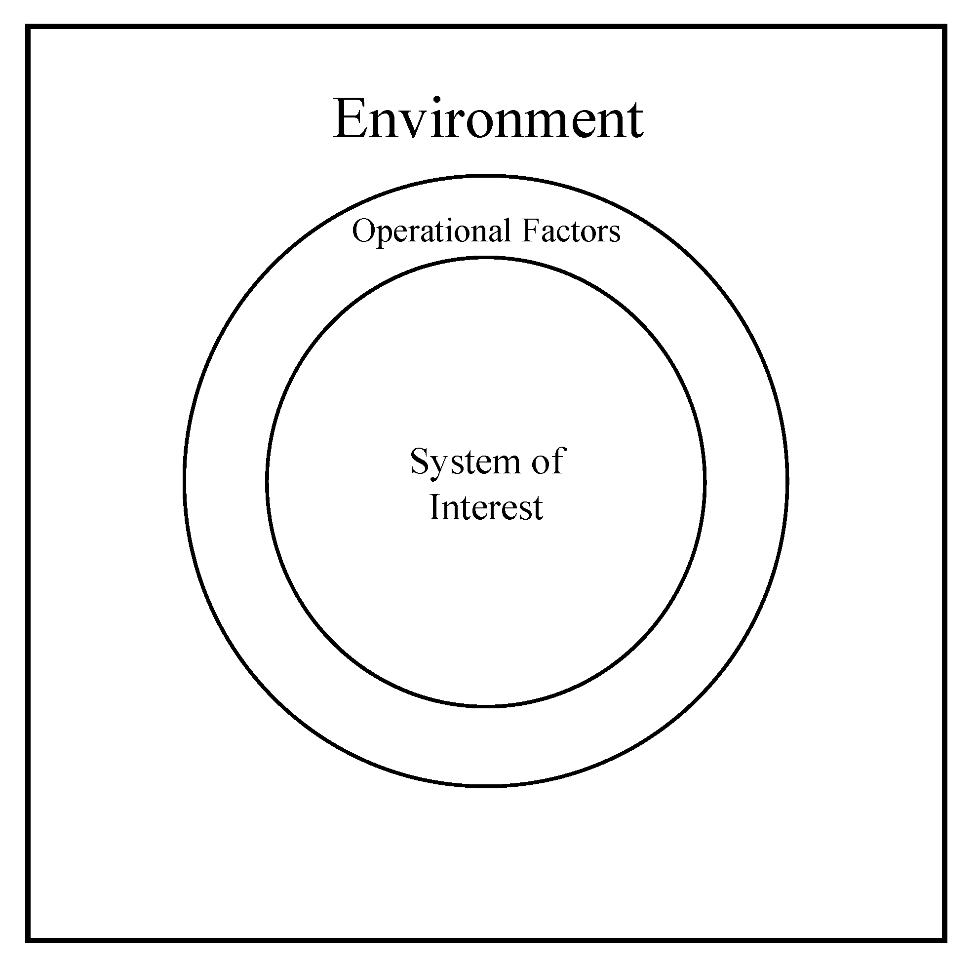
The conditions of a scenario are either controllable by humans, such as technologies and organizational structures, or uncontrollable, such as the weather, terrain, and temperature of the operational landscape. To illustrate the ideas presented in this paper, we specifically list uncontrollable, non-numeric scenario factors for military studies. For instance, knowledgeable participants about military maneuver would specify different terrain types.

2.3.2. Ranking the Non-Numeric Values of Scenario Factors

Non-numeric, unordered values greatly diminish the advantage of applying efficient DOE, i.e., the value combinations would be arbitrary and have no real meaning for selecting an appropriate subset of combinations that will mathematically support a global optimum [28]. At times, subject matter experts (SME) assign a rank order based on direct elicitation, which simply places each factor value on a line from 1 to 100. However, direct elicitation is replete with flaws for capturing the actual order of importance [29]. We select two techniques because of their applicability to different study conditions: (1) Analytic Hierarchical Process and (2) Failure Mode, Effects, and Criticality Analysis.

The Analytical Hierarchy Process (AHP) develops a hierarchy for a set of elements [30]. The first step identifies the values that the non-numeric factor can assume. The second step calls on the expertise of the participants to assign an AHP score for each pairwise comparison of values within each factor [31]. Each paired comparison between two values results in exactly one of several conclusions from

Table 2. AHP scores for pairwise comparison of importance, adapted from Taderhoost [31].

Score for AHP	Comparative Importance
1	Equally Important
2	Equally to Moderately Important
3	Moderately Important
4	Moderately to Strongly Important
5	Strongly Important
6	Strongly to Very Strongly Important
7	Very Strongly Important
8	Very Strongly to Extremely Important
9	Extremely Important

, which is adapted from Taderhoost’s original work [31].

Expert participants determine the conclusion for each pairwise comparison of values. For instance, a score of “5” in comparing B with D means that B is “Strongly Important” over D. Reciprocally, a comparison of D with B results in a score of “1/5” with an inverse meaning to a score of “5.” The complete set of pairwise comparisons is designated as matrix A.

A consistency check of the resultant pairwise comparison matrix is important to validate the prioritization. Consistency refers to the experts’ logical assignment of the scores, i.e., if Mountain is preferred over Desert and Jungle is preferred over Mountain, then Jungle should be preferred over Desert. Eigenvector computations determine the consistency of matrix A [30,32]. The consistency ratio is calculated from the maximum Eigen value (λ_max) of matrix A, and the random index (RI) obtained from Saaty’s [30] tables. If λ_max/RI is lower than 0.10, then the resulting rankings are reasonable [30].

We discuss the AHP with an example that considers a scenario to test a new, individually carried radio system. SME develop a comparison matrix, A (bordered, shaded area), for values that the scenario factor, operational terrain, can assume (

Table 3. Example comparison matrix for a scenario’s operational terrain.

Column Compared with Row	Desert	Mountain	Jungle	Urban
Desert	1	7	5	9
Mountain	1/7	1	1/3	4
Jungle	1/5	3	1	7
Urban	1/9	1/4	1/7	1
Summed Scores	1.45	11.25	6.48	21.00
Final Ranking (High is Best)	1	3	2	4

). Eigen value computations is left to the reader [32]. The computed consistency ratio from matrix A in this example is <0.10 and is therefore logically consistent [30]. The sum score of each column determines how to rank each factor value as shown in the last row of Table 3. The final rankings (high is best or most important) suggest that urban is the most important terrain type to test an individually carried radio system.

AHP is useful for rank ordering a relatively small number (<10) of non-numeric factor values. However, pairwise comparisons of more than nine elements are impractical. The following section is an approach for comparing more than 10 elements.

Failure mode, effects, and criticality analysis (FMECA) is a second approach to rank order non-numeric factor values based on their criticality to stressing the system. This approach is adapted from system reliability analysis. FMECA is a design technique to study how subsystem failures may affect the rest of the system [33]. Determining the criticality of any specific subsystem failure consists of three scores: severity, frequency, and detection probability. Severity is the seriousness of the failure’s impact on the system. Frequency is how often the failure occurs, regardless of manner. Detection probability is the likelihood that the failure will be detected before it has catastrophic effects on the system. For the purposes of this work, the detection score is not applicable and is therefore shaded in gray. Each element of an FMECA score ranges from 1–10 (

Table 4. FMECA scoring levels.

Severity	Score	Frequency	Score	Detection	Score
Minor	1	Minor	1	Very High	1–2
Low	2–3	Low	2–3	High	3–4
Moderate	4–6	Moderate	4–6	Moderate	5–6
High	7–8	High	7–8	Low	7–8
Very High	9–10	Very High	9–10	Very Low	9
				Absolute Certainty of # Detections	10

). A failure’s criticality score is the product of all three scores. In this paper, only Severity and Frequency are multiplied. We submit that the criticality score of a factor value for achieving the goals of a study is a credible means to rank order values.

We again consider the factor values of the operational terrain: desert, mountain, jungle, or urban. The expert participants review the objectives for testing an individually carried radio and score the factor’s value on the ability to stress the radio. For instance, the experts may consider that “urban terrain” has a highly negative impact (stress) on the radio transmission, thereby assigning a score of 8 for severity. If the concept of operations for the radio indicates that the radio will routinely be used in an urban environment, then the experts may rate frequency a 10. Therefore, the criticality score for urban is 8 × 10 = 80. Criticality scores for the remaining terrain values may result in the rankings shown in

Table 5. Criticality scores of terrain values for testing the individually carried radio.

Operational Terrain	Severity	Frequency	Criticality Score	Rank
Desert	4	5	20	1
Mountain	7	6	42	2
Jungle	8	6	48	3
Urban	8	10	80	4

.

Rank ordering the factor values enables the use of DOE. After discretizing the factor values with either AHP or FMECA, expert participants may treat the factor as numeric and frame the problem space into unique combinations of the factor values. It is possible to rank order a magnitude more factor values with FMECA than AHP. Consequently, the number of future scenarios also increases, and the role of an efficient DOE becomes clear.

2.3.3. Identifying an Efficient Set of Scenario Designs

The diversity of scenarios that can be imagined range from those that the social sciences community would create, as well as scenarios formulated by the math and engineering sciences. This combinatorial issue is the same challenge for many experimenters [18]. In recent decades, there has been great advances in improving DOE to efficiently examine complex problems. Efficiency in DOE refers to minimizing the design points (scenarios) to explore while gaining the most information [34]. Foremost in these new experimental designs are nearly orthogonal Latin hypercubes (NOLH).

As Hernandez, Lucas, and Carlyle [35] explain, when using lattice sampling [36], a DOE with k factors and n values for each factor, results in a Latin hypercube that is n x k in size. The factor values in the lattice are 1 to n and basically act as ordered ranks. The number of possible scenarios is (n!)^k−1. However, the new methods for constructing experimental designs can specify a much smaller subset of design points that will gain the most information from the problem space. For instance, Cioppa and Lucas [28] show that an NOLH design can efficiently examine seven factors, each assuming 17 different values.

Consider three (3) critical scenario factors: terrain, friendly organizational makeup, and enemy rules of engagement. Notionally, the scenarios are being developed to test a new motorized vehicle.

Table 6. An efficient 3 × 8 experimental design [35].

Scenario	Scenario Factors (k from 1 to 3)
	k1	k2	k3
Scenario 1	1	2	1
Scenario 2	6	7	3
Scenario 3	2	5	6
Scenario 4	4	8	4
Scenario 5	3	6	7
Scenario 6	8	4	5
Scenario 7	7	3	2
Scenario 8	5	1	8

is an NOLH design to examine three factors, each able to assume eight different values [35]. Each row is a design combination for a new scenario. In viewing the DOE structure, we can see the relationship with Zwicky’s morphological box [13,14,17]. Experimenters replace the rank shown in the design with the appropriate factor value to complete the design matrix for the simulation runs. For instance, if k1 is Terrain, subject matter experts may rank the factor values from most passable, rank #1, to least passable, rank #8. The assigned ranks could be: 1 = Open, 2 = Oasis, 3 = Desert, 4 = Steppe, 5 = Tundra, 6 = Forest, 7 = Hill, and 8 = Swamp. Thus, creating a scenario within a “Swamp” will likely stress the motorized vehicle the most.

3. Deriving Metamodels from Scenario-Based Computer Experimentation

The series of techniques that have been discussed may be employed to develop mathematical equations for the uncontrollable variables, which can then be used to assist in defining the solution space of a complex systems problem. The construction of these scenarios and the ensuing computer runs provide data that supports statistical analyses to determine the variables or factors with the most impact on a measure of interest. Importantly, the DOE are highly effective in identifying critical interactions among the factors. These interactions track the emergent behaviors that the system exhibits and to which systems engineers pay particular attention in developing solutions. Furthermore, experimentation provides an ability to identify scenario conditions that maximize or minimize a measure of interest [37].

Implementing the DOE-enhanced scenarios in a computer simulation results in metamodels for the solution space of the problem [38]. The metamodel is a mathematical expression for the response surface of the solution space created from the variables. In computer simulations, a mathematical expression from the results of a simulation is a metamodel since the simulation is already a model or abstract of real things [38]. Figure 3 illustrates the response surface for a measure of interest, f(X), that is affected by two variables, X₁ and X₂.

Each measure of interest in the problem has a metamodel. Ergo, there is an equation based on significant variables (controllable and uncontrollable) for each measure. The equations would take a similar form to Equation (1), where M1 is the measure of interest and the significant variables are x and k. The coefficients (β) are estimates for the degree that the variables x, k, and the interaction, xk, influences the behavior of M1. We note that the resultant equation from an experimental design is a linear equation and can be shown to have an optimal solution [39].

$$M1={\widehat{\beta }}_0+{\widehat{\beta }}_1{x}^{-2/3}+{\widehat{\beta }}_2{k}^{-1/3}+{\widehat{\beta }}_3{(xk)}^{-2/3}$$

(1)

The objective function could be an aggregate of the mathematical transformation of each measure of interest, along with any other considerations in the problem. Each metamodel derived from experimentation would be one constraint equation. These constraint equations would be added to previous constraints about the problem, along with the objective function. The idea is to bound the problem such that the feasible region is formed as the example in Figure 2. The overall result is a set of linear constraint equations, which optimization techniques would aim to solve [3,12,15].

As a point of emphasis, discretizing the scenario factors in the manner shown in this paper provides an advantage for defining the solution space. A linear program (LP) is an optimization routine that consists only of continuous variables and linear equations. LPs are proven to have an optimal solution [12].

Transforming the non-linear nature of the theoretical response surface can be of concern. Mayhap the set of linear equations have not accurately captured the feasible region. Long and continued studies in LP provide assurance that a solution from LP approximation of the solution space is credible and has utility beyond a singular answer. As Bazaraa et al. [12] explain, linear programming is one of the most extensively used mathematical models to solve a wide array of problems. In many instances, LP is applied to non-linear problems through a sequence of piece-wise linear equations. It is an essential tool for many complex problems [12,40].

When some variables in an LP are discrete or integer, the optimization routine is a mixed integer program (MIP). A MIP is a subset of LP and also proven to have an optimal solution but is restrictive in the solution because of the requirement to have some variables assume only integer values. When the problem has only integer variables, it is an integer program (IP) and comes with its inherent restrictions. Still more restrictive are binary integer programs (BIP) where the variables may take only the values of zero or one. For a BIP, the solution space is much smaller than an LP [40]. In short, as restrictions on the variables increase, the solution space decreases.

To be considered in a mathematical equation, non-numeric scenario factors are transformed into binary variables, thus considerably shrinking the LP solution space. For instance, consider “Desert” as a value for the operational terrain factor. To mathematically include it in the scenario, a “dummy variable” is used to designate if the factor value is present, i.e., “Desert” would assume a value of one and all other dummy variables for the factor would be assigned a value of zero [41]. On the other hand, discretizing the operational terrain factor values in rank order results in an IP or MIP, which is a larger feasible region than one from a BIP [40]. Avoiding a BIP supports the need to bound the problem while keeping the solution space as large as possible.

4. Steps for Defining Boundaries

The series of methods from the previous section outlines a systematic process to define the critical, uncontrollable, non-numeric variables in a complex system [10,11]. Establishing the important factors of the problem and expressing them within a set of linear equations moves toward a completely defined solution space.

4.1. Boundary Development for a Complex Systems Problem

The sequence of activities in Figure 4 for defining the boundaries of a complex system of interest is a notional approach that a practitioner can take. The authors recognize that some steps such as developing measures consist of many well-known methods. It is not the authors’ intent to dictate how each step in Figure 4 is accomplished. After gaining an in-depth understanding of the problem, the scientist or engineer identifies relevant measures and defines a finite, but not necessarily small set of scenario factors or variables. As this paper emphasizes, uncontrollable, non-numeric variables are the focus of the techniques previously described. Next, the values that the variables can assume are established. If a variable is non-numeric, the authors have introduced a novel use of AHP or FMECA to discretize the values. To reduce the number of scenarios to explore, the scientist would employ an efficient experimental design in a computer simulation. Examination of the problem space for each measure of interest enables analysts to use output data to develop a linear expression for each measure.

The authors recognize that Step 9, formulating a complete optimization problem, requires work in understanding all elements of the problem. Constraint equations and the objective function from Steps 1–8 are examined by the scientists and analysts for their utility in the overall problem. The approach that has been discussed focused on the variables that are difficult to quantify but are significant in solution development. By developing a means to create mathematical expressions from uncontrollable scenario factors, the scientist can help define the full problem from which credible solutions may be found.

4.2. Applying Steps 1 through 5—Boundary Development for a Complex Systems Problem

We illustrate how a subset of the steps in the previous approach may be applied to the study of a LAES system [22]. The initial LAES work involved expert participants who had established the study objectives, measures, and variables of interest in the problem. We begin at Step 4. Among the variables are two non-numeric scenario factors. For designing a LAES system, engineers must consider the geographical areas for the storage system and the sophistication of technology in the available infrastructure. The geographical area limits the type of technology that can be applied. For instance, hydro powered technologies benefit from areas with elevation changes. The level of sophistication in the infrastructure can dictate the solutions for a storage system. Additionally, a pipeline infrastructure benefits gas generation, while geothermal technologies require several layers of conversion and transfer from the ground to be used on the expansion side of the LAES system. There is a need to discretize the scenario space with these two scenario factors.

The values that each factor can assume follow: Geography—Flat Terrain, Rolling Terrain, or High Altitude (Mountainous); Technology—Hydro, Gas Powered, or Geothermal. We rank the values for the factors using AHP as Taherdoost [31] describes.

Table 7. Comparison matrix for technology values in a LAES system design environment.

Column Compared with Row.	Hydro	Gas	Geothermal
Hydro	1	5	1/3
Gas	1/5	1	1/7
Geothermal	3	7	1
Total Column Score	4.20	13.00	1.48
Rank Order (high is best)	2	3	1

presents the pairwise matrix for Technology. The total scores for each value level of Technology show that the rank order from best to worst is Gas, Hydro, and Geothermal. Similarly, Geography’s rank order is Rolling Terrain, Flat Terrain, and High Altitude from best to worst, respectively, and where a score of 3 is best.

Table 8. An experimental design for possible scenarios to design a LAES system.

Scenario	Scenario Factors for LAES System Design
	Technology	Geography
Scenario 1	Geothermal (1)	High Altitude (1)
Scenario 2	Geothermal (1)	Flat (2)
Scenario 3	Geothermal (1)	Rolling Hills (3)
Scenario 4	Hydro (2)	High Altitude (1)
Scenario 5	Hydro (2)	Flat (2)
Scenario 6	Hydro (2)	Rolling Hills (3)
Scenario 7	Gas (3)	High Altitude (1)
Scenario 8	Gas (3)	Flat (2)
Scenario 9	Gas (3)	Rolling Hills (3)

presents a full factorial experimental design [41] for the possible conditions in which participants would develop a design solution for a LAES system. An examination by the expert participants for the feasibility of the scenarios could find that Scenario 5 is not plausible since Hydro systems are more advantageous in terrain with elevation changes. However, the participants may still wish to consider such an environment if they would like to explore using water tower generation technologies. The expert participants may also identify Scenario 1 as the least desirable situation to develop a LAES system design and decide to remove the scenario for consideration. Based on their expert judgment, the panel may include or exclude any scenario. Analyses may also show that there is no significant interaction between Technology and Geography for this problem. Therefore, this interaction term would not be in a constraint equation.

The next iteration of the LAES study would model the scenario in an appropriate modeling and simulation environment. Experimentation on the potential design solutions would enable analysis of the output data and development of appropriate mathematical equations for the given measures in the problem. Incorporating the new equations into a larger set of equations would support an optimal set of values for the scenario variables. It is also possible to isolate a measure and examine the DOE to identify a set of acceptable designs and critical design parameters to optimize the specific measure [37]. In fact, the original LAES system study used an experimental design that included air flow rate and compression pressure as factors to develop design parameters for a LAES system [42,43]. However, those experiments were run in a lab setting that did not consider the scenario factors in Table 8. Placing the original LAES experiments in the different scenarios in Table 8 provides a more robust solution. For Steps 6–9, the LAES study team would create a database for all variables in the original LAES study and the scenario factors in Table 8 in an appropriate simulation model. Experimentation results would enable construction of linear equations that may be used as part of an optimization model.

5. Conclusions

Complex systems problems are often inundated with non-numeric, uncontrollable variables. Poorly defined solution spaces can result in infinite or no solutions. Conversely, overly constrained solution spaces may yield few design solutions. Consequently, investigating these types of system variables are a challenge to engineers and analysts. Ultimately, the idea is to determine how non-numeric, uncontrollable variables fit in the design solution. Focusing on computers and simulation models as the primary tools, the authors have developed a methodical approach to credibly shape the design space in terms of these difficult variables.

Using GMA as a basis, this work has outlined a way to study uncontrollable, non-numeric variables. A prevalent issue for employing GMA is the near uncountable number of scenarios that could exist in the problem space. To address this combinatorial issue, the authors advocate using advances in DOE. However, to gain the benefits that DOE offers, requires a numerical hierarchy for the factor values. Yet, non-numeric factors by definition do not have a hierarchy. This work presents an approach for discretizing the scenario factors of the problem space, thereby simplifying scenario generation and reducing the number of scenarios to be examined. Each value of a non-numeric scenario factor is ranked in order of importance as defined by the study participants in one of two ways: AHP [30] or FMECA [33]. For problem spaces with many factors and value levels, advanced and customized designs of experiments are available [21]. If the number of factors and values are not large in number, then simpler experimental designs are adequate [41]. The final step of a scenario-based computer experiment results in mathematical expressions that contain difficult variables in the problem space and relate them to different measures of interest. The intent is to use the resultant equations to augment other equations that engineers and analysts have developed to bound the problem.

This paper does not attempt to develop system design solutions or manage system configuration. The ideas of this study are offered only to define the feasible space of a complex problem. The subject matter experts, stakeholder(s), scientist, and analysts may determine which of the resulting constraint equations make the most sense for the problem. Afterward, statistical and optimization methods may be employed to generate one or more credible solutions. The theoretical foundations of optimization routines are well-established [9,12,40]. Other techniques from many disciplines to develop a solution from the design space or solution space, are also plentiful and well-founded. Employing those techniques is beyond the scope of this paper. It suffices to say that the paper provides the foundation to develop solutions from a credibly formed problem space.

References

1. Andrew, P.; James, E. Introduction to Systems Engineering; Wiley: New York, NY, USA, 2000. [Google Scholar]
2. Kossiakoff, A.; Sweet, W.N.; Seymour, S.J.; Biemer, S.M. Systems Engineering Principles and Practice; Wiley: New York, NY, USA, 2011. [Google Scholar]
3. Vanderbei, R.J. Linear Programming: Foundations and Extensions, 2nd ed.; Springer: New York, NY, USA, 2001. [Google Scholar]
4. Summers, J. Reasoning in Engineering Design. In Proceedings of the Volume 5a: 17th International Conference on Design Theory and Methodology; American Society of Mechanical Engineers: New York, NY, USA, 2005; pp. 329–340. [Google Scholar]
5. INCOSE. Systems Engineering Handbook, 4th ed.; Wiley: New York, NY, USA, 2015. [Google Scholar]
6. Wasson, C.S. Systems Engineering Analysis, Design, and Development, 2nd ed.; John Wiley & Sons: Hoboken, NJ, USA, 2016. [Google Scholar]
7. Langford, G.O. Engineering Systems Integration: Theory, Metrics, and Methods; CRC Press: Boca Raton, FL, USA, 2012. [Google Scholar]
8. ANSI/EIA. Processes for Engineering A System; ANSI/EIA 632-2003American National Standards Institute (ANSI)/Electronic Industries Association (EIA): Philadelphia, PA, USA, 2003. [Google Scholar]
9. Winston, W.L. Operations Research: Applications and Algorithms; Brooks-Cole: Toronto, ON, Canada, 2004. [Google Scholar]
10. Mingers, J. Combining IS Research Methods: Towards a Pluralist Methodology. Inf. Syst. Res. 2001, 12, 240–259. [Google Scholar] [CrossRef] [Green Version]
11. Creswell, J.W.; Creswell, J.D. Research Design, 5th ed.; SAGE Publication Inc.: Los Angeles, CA, USA, 2018. [Google Scholar]
12. Bazaraa, M.S.; Jarvis, J.J.; Sherali, H.D. Linear Programming and Network Flows, 4th ed.; John Wiley & Sons: New York, NY, USA, 2004. [Google Scholar]
13. Zwicky, F. Discovery, Invention, Research—Through the Morphological Approach; The Macmillan Company: Toronto, ON, USA, 1969. [Google Scholar]
14. Ritchey, T. Fritz Zwicky, ‘Morphologie’ and Policy Analysis. In Proceedings of the 16th EURO Conference on Operational Analysis, Brussels, Belgium, September 1998; Available online: https://www.researchgate.net/profile/Tom-Ritchey/publication/267794873_Fritz_Zwicky_Morphologie_and_Policy_Analysis/links/551aaa400cf2bb754076a92d/Fritz-Zwicky-Morphologie-and-Policy-Analysis.pdf (accessed on 19 December 2021).
15. Alvarez, A.; Ritchey, T. Application of General Morphological Analysis from Engineering Design to Policy Analysis. Acta Morphol. Gen. 2015, 4, 1–40. [Google Scholar]
16. Ritchey, T. Modeling Alternative Futures with General Morphological Analysis. World Futur. Rev. 2011, 3, 83–94. [Google Scholar] [CrossRef] [Green Version]
17. Buede, D.M. The Engineering Design of Systems, Models and Methods; John Wiley & Sons, Inc.: Hoboken, NJ, USA, 2016. [Google Scholar]
18. van Kouwen, F.; Dieperink, C.; Schot, P.P.; Wassen, M.J. Computer-Supported Cognitive Mapping for Participatory Problem Structuring. Environ. Plan. A 2009, 41, 63–81. [Google Scholar] [CrossRef]
19. Ritchey, T. Problem Structuring Using Computer-Aided Morphological Analysis. J. Oper. Res. Soc. 2006, 57, 792–801. [Google Scholar] [CrossRef]
20. Badal, M.A. Strategic Management: Methods and Models. Master’s Thesis, DTU, Technical University of Denmark, Lyngbyc, Denmark, 2006. [Google Scholar]
21. Lucas, T.W.; Kelton, D.W.; Sanchez, P.J.; Sanchez, S.M.; Anderson, B.L. Changing the Paradigm: Simulation, Now a Method of First Resort. Naval Res. Logist. 2015, 62, 293–303. [Google Scholar] [CrossRef]
22. Girouard, C.; Pollman, A.G.; Hernandez, A.S. Modeling and Simulation Informed Conceptual Design, Analysis, and Initial Component Selection of a Supply-Side Building Scale LAES System for Renewable, Islanded Microgrid Resiliency. In Proceedings of the 87th Military Operations Society Symposium, Colorado Springs, CO, USA, 17–20 June 2019. [Google Scholar]
23. Chermak, T.J. Scenario Planning in Organizations: How to Create, Use, and Assess Scenarios; Berrett-Koehler Publishers, Inc.: San Francisco, CA, USA, 2011. [Google Scholar]
24. Lindren, M.; Bandhold, H. Scenario Planning: The Link between Future and Strategy; Palgrave McMillan: London, UK, 2009. [Google Scholar]
25. von Reibnitz, U. Scenario Techniques; McGraw-Hill Publishing Co: New York, NY, USA, 1988. [Google Scholar]
26. Mietzner, D.; Reger, G. Advantages and Disadvantages of Scenario Approaches for Strategic Foresight. Int. J. Technol. Intell. Plan. 2005, 1, 220–239. [Google Scholar] [CrossRef] [Green Version]
27. Perla, P.P.; Curry, J. The Art of Wargaming: A Guide for Professionals and Hobbyists; U.S. Naval Institute Press: Annapolis, MD, USA, 2011. [Google Scholar]
28. Cioppa, T.M.; Lucas, T.W. Efficient Nearly Orthogonal and Space-Filling Latin Hypercubes. Technometrics 2007, 49, 45–55. [Google Scholar] [CrossRef]
29. Watson, S.R.; Buede, D.M. Decision Synthesis: The Principles and Practice of Decision Analysis; Cambridge University Press: Cambridge, UK, 1987. [Google Scholar]
30. Saaty, T.L. The Analytic Hierarchy Process: Planning, Priority Setting, Resources Allocation; McGraw-Hill: London, UK, 1980. [Google Scholar]
31. Taherdoost, H. Decision Making Using the Analytic Hierarchy Process (AHP); A Step by Step Approach. Int. J. Econ. Manag. Syst. 2017, 2, 244–246. [Google Scholar]
32. Leon, S.J. Linear Algebra with Applications; Prentice Hall: Upper Saddle River, NJ, USA, 2002. [Google Scholar]
33. Blanchard, B.S.; Fabrycky, W.J. Systems Engineering and Analysis, 5th ed.; Pearson Prentice Hall: Upper Saddle River, NJ, USA, 2011. [Google Scholar]
34. Kleijnen, J.P.C.; Sanchez, S.M.; Lucas, T.W.; Cioppa, T.M. A User’s Guide to the Brave New World of Designing Simulation Experiments, INFORMS. J. Comput. 2005, 18, 263–289. [Google Scholar]
35. Hernandez, A.S.; Lucas, T.W.; Sanchez, P.J. Selecting random Latin hypercubes dimensions and designs through estimation of maximum absolute pairwise correlation. In Proceedings of the 2012 Winter Simulation Conference, Berlin, Germany, 9–13 December 2012. [Google Scholar]
36. Patterson, H.D. The Errors of Lattice Sampling. J. R. Stat. Society Series B Methodol. 1954, 17, 140–149. [Google Scholar] [CrossRef]
37. Koehler, J.R.; Owen, A.B. Computer Experiments. In Handbook Statistics; Ghosh, S., Rao, C.R., Eds.; Elsevier Science: New York, NY, USA, 1996; Volume 14, pp. 261–308. [Google Scholar]
38. Law, A.M. Simulation Modeling and Analysis, 5th ed.; McGraw-Hill Education: New York, NY, USA, 2015. [Google Scholar]
39. McKay, M.D.; Beckman, R.J.; Conover, W.J. A Comparison of Three Methods for Selecting Values of Input Variables in the Analysis of Output from a Computer Code. Technometrics 1979, 22, 239–245. [Google Scholar]
40. Wolsey, L.A. Integer Programming; John Wiley& Sons Inc.: New York, NY, USA, 1998. [Google Scholar]
41. Montgomery, D.C. Design and Analysis of Experiments, 5th ed.; Wiley: New York, NY, USA, 2005. [Google Scholar]
42. Willis, R.; Pollman, A.G.; Gannon, A.J.; Hernandez, A.S. Modeling a Building Scale Liquid Ari Energy Storage and Expansion System with ASPEN HYSYS. In Proceedings of the 3rd IEEE International Conference on DC Microgrids (ICDCM), Matsue, Shimane, Japan, 20–23 May 2019. [Google Scholar]
43. Howe, T.; Pollman, A.G.; Gannon, A.J. Operating Range for a Combined, Building-scale Liquid Air Energy Storage and Expansion System: Energy and Exergy Analysis. Entropy 2018, 20, 770. [Google Scholar] [CrossRef] [PubMed] [Green Version]
Figure 1. System of interest and factors for consideration.
Systems 09 00089 g001
Figure 2. Several ways to represent constraints that define the feasible region in a linear programming problem.
Systems 09 00089 g002
Figure 3. Response surface for measure of interest as described by variables X1 and X2.
Systems 09 00089 g003
Figure 4. Capturing the steps to formulate the boundaries of a systems problem.
Systems 09 00089 g004