Mathematical Modeling for Predicting Growth and Yield of Halophyte Hedysarum scoparium in Arid Regions under Variable Irrigation and Soil Amendment Conditions

Abstract

Growing degree days (GDDs) and leaf area index (LAI) greatly influence the growth and yield of many crops grown in arid regions. Therefore, variation in LAI due to GDD can provide a theoretical basis for predicting crop growth, water consumption, plant development, and yield in arid agriculture via the development of mathematical growth models. This study described the relationship between plant biomass production and variation in LAI due to GDD in arid regions under different types of irrigation (fresh water and saline water) and soils amended with different substances (manure+sandy soil, compost+sandy soil, clay+sandy soil, and sandy soil). Mathematical models for LAI were established for GDDs. In addition, different water quality irrigation techniques were used as independent variables to calculate the LAI of halophytic plants (Hedysarum scoparium) in arid regions under different soil amendment treatments. Furthermore, mathematical models for plant biomass production were developed by using the LAI and GDDs. For this purpose, Logistic, Gaussian, modified Gaussian, and Cubic polynomial models were used. Modified Gaussian and Cubic polynomial models are the best among all developed models, but Cubic polynomial models are more suitable among all developed models because of their simple quadratic equations that can be solved by using the first derivative. It was observed that with increased salt concentration in the irrigation water, the growth of per plant production decreased. However, soil amendments like manure and compost enhance salt tolerance against salt stress and enable plants to sustain their growth. Furthermore, Hedysarum scoparium attains maximum LAI when its GDD is about 1117.5 °C under both irrigation regimes and in all soil amendment treatments. It was concluded that these predicted mathematical models can provide crucial insights for enhancing production in arid regions by using eco-friendly soil amendments to improve water use efficiency across diverse types of water irrigation.

1. Introduction

Fresh water scarcity and soil salinization are the main issues that restrict agriculture production in arid and semi-arid regions all over the world [1]. The primary reason for lower agricultural production in arid and semi-arid regions is the high evaporation rate caused by higher temperatures and lower rainfall [2]. Most arid regions have a large amount of underground saline water resources. These water resources have huge agricultural potential and can meet the water demands of the agricultural sector in arid regions [3]. These days, many researchers use saline water resources to grow many valuable crops such as wheat, cotton, and rice in arable land regions. They are investigating their responses in terms of yield, growth development, water use efficiency, and saline water effects on soil physical and chemical properties [4,5,6]. In arid regions, there is a lack of research on utilizing saline water resources for agricultural production due to higher temperatures and nutrient-deficient soil [7]. The soil conditions in arid and semi-arid regions are typically dry, with fewer nutrients and a sandy structure. Soil erosion and wind erosion contribute to restricting plant growth in arid regions because of degraded soil structure [8]. Limited research has explored the application of saline water for irrigating desert plants and halophyte plants in dry land regions. Certain studies have noted that, despite the minimal water quality needs of desert and halophyte flora, salt buildup resulting from saline water irrigation can hinder plant growth and, in severe cases, result in plant mortality [9,10]. Therefore, the crucial aspect of effectively utilizing saline water lies in mitigating the harm inflicted on plants due to salt accumulation in the soil.

Soil amendments are considered the most important and eco-friendly technique in arid and semi-arid regions to stabilize sandy soil and promote plant growth [11]. Soil amendments with organic and inorganic materials are helpful for improving soil properties and providing a favorable environment for plant development. Many organic and inorganic materials have been used as soil amendments, such as gravel, gypsum, and clay for inorganic materials, and biochar, manure, and compost for organic materials [12,13]. Among all these materials, clay, manure, and compost are considered eco-friendly and cast-effective soil amendments [14]. Despite this eco-friendly control of wind erosion by these soil amendment materials, they also enhance organic matter in the soil, increase water holding capacity, and reduce water infiltration [13]. However, the effects of these soil amendments on halophyte plant growth and development under saline conditions are still inadequate.

It is well established for many crops that yield and biomass growth are intricately linked to their leaf area index (LAI) [15]. The LAI significantly influences biomass accumulation and transpiration, while the partitioning of biomass affects yield. Additionally, LAI serves as a critical variable in various process models, such as evapotranspiration and canopy photosynthesis. LAI impacts the size of the plant–atmosphere interface. This role is crucial in the exchange of energy and mass between the canopy and the atmosphere [16]. During the initial stages of the growing season, LAI remains low and increases gradually. However, as the season progresses, LAI experiences a rapid increase, reaching its peak before the leaves begin to senesce and the plants reach physiological maturity [17]. Analyzing trends in LAI can offer valuable technical insights for simulating dynamic changes in biomass and yields. Several techniques have been developed to predict LAI, including crop simulation models and generic crop models [18,19,20].

For an ideal simulation model of LAI and biomass, several input parameters are necessary. The model should be grounded in the underlying physiological and phenological processes observed in real plants [21]. Two approaches to address this challenge are estimation methods and species-specific growth models [21]. Estimation methods rely either on remote sensing or direct measurements to assess LAI [22,23]. In contrast, species growth models are established on theoretical foundations, such as the Logistic model, Gompertz model, Richards model, and Chanter model [15,17,20]. These models utilize one or more parameters to represent physical properties and describe how population sizes and biomass evolve over time. The logistic model is a classic population model that has been extensively utilized for simulating population growth with a commendable level of accuracy [16,24].

Growing degree days (GDDs) are another crucial meteorological factor that influences various crop growth indices, including plant height, leaf area index, biomass, and harvest index [16,24,25,26,27]. GDDs use normalized logistic models for crops such as potato, winter wheat, summer maize, rice, and cotton, based on comprehensive studies across over 50 regions in China. These models utilized GDDs as a key variable to analyze crop growth dynamics.

Although the logistic growth model is effective in predicting plant growth during certain periods, its accuracy decreases when forecasting growth in the later stages and during periods of decline. To address this limitation, alternative mathematical models have been explored. These include the Gaussian model, Cubic polynomial model, modified Gaussian model, and Log-normal model, which offer improved accuracy in predicting plant growth across various stages [16,24]. However, it is worth noting that these models have primarily been developed and applied to crops such as cotton [28], wheat, sesbania, cluster bean [20], and maize [29] to anticipate growth under diverse environmental conditions. Meanwhile, there is a lack of studies examining the applicability of these models to halophyte plants in desert conditions.

Hedysarum scoparium Fisch. et Mey. is an important halophyte shrub species. It is extensively distributed in arid and semi-arid regions [30]. This species, characterized by its tall stature and spring flowering, can reach heights of up to 5 m [31]. The dispersal unit of Hedysarum scoparium is a large pod containing several seeds. It exhibits rapid growth and high resistance to drought, salinity, and temperature [32].

Hedysarum scoparium is valued for its economic and ecological significance, being used for livestock fodder, water and soil conservation, and sand dune stabilization [31].

The aim of this study was to develop and assess a method for simulating leaf area index (LAI) and biomass of Hedysarum scoparium, utilizing selected mathematical models under varied irrigation and soil amendment conditions. Additionally, the impact of various soil amendments on maximum LAI under different qualities of irrigation was investigated. The maximum fresh weight biomass per square meter (m²) was estimated using LAI based on Michaelis–Menten kinetics. Finally, a mathematical model for simulating Hedysarum scoparium biomass, incorporating LAI and GDD, was formulated under different soil amendment treatments.

2. Materials and Methods

2.1. Field Conditions

A field experiment was conducted at the Sindh Engro Coal Mining Company experimental site in Tharparkar, Block II, located 10 km away from Islamkot, Tharparkar, Sindh, Pakistan. The experiment spanned from 10 November 2023 to 13 March 2024. The experimental site experiences extreme weather conditions, characterized by long, hot summers, with maximum temperatures reaching nearly 48 °C, and short winters, with minimum temperatures dropping to nearly 8 °C. The experimental site’s annual precipitation is approximately 100 mm, with an annual evaporation rate of 2600 mm. The soil at the experimental site is predominantly dry sandy soil, with minimal nutrient content [20].

2.2. Experimental Design

Three types of soil amendment materials (manure, compost, and clay) were used in a completely randomized block design. Manure, compost, and clay were added to sandy soil in plots 2.6 m² in size at a rate of 5.7 kg per plot. Each soil amendment treatment contained six replicates. Additionally, six plots consisted of sandy soil, serving as the control treatment. Seeds of the halophytic plant Hedysarum scoparium were sourced from China for experimental study in the Tharparkar of Pakistan. Carefully selected healthy seeds of equal size were planted in the experimental field, following a completely randomized block design with six replicates for each soil amendment treatment. Plant spacing was maintained at 0.3 m within plants and 0.2 m within rows of each plot. The experimental design and the location in the field have been depicted in Figure 1.

Before sowing the seeds, the field underwent preparation, which involved the application of urea fertilizer at a rate of 240 kg·ha⁻¹, as recommended by studies [33]. During the germination and seedling establishment phase, fresh water was provided for a duration of 20 days. To assess the impact of saline water irrigation on the growth of Hedysarum scoparium, under soil amendment treatments, irrigation commenced 20 days after seed sowing. One set of these four soil amendment treatments with three replicates received saline water, while another group was irrigated with fresh water, serving as the control, also with three replicates for each soil amendment treatment. The physical and chemical properties of both fresh water and saline water used in the experiment are detailed in

Table 1. Water quality parameters.

Water Quality	EC (dS·m−1)	Total Dissolved Solids (ppm)	Nitrate (ppm)	Nitrite (ppm)	Chloride (ppm)	Fluoride (ppm)	Manganese (ppm)
Saline water	4.368	6240	0.4	0.002	2231.03	1.15	0.006
Fresh water	0.357	510	0.4	0.015	196.75	0.35	0.006

Note: EC = electrical conductivity.

.

The irrigation process utilized a drip irrigation system, with a water meter installed on the primary irrigation pipeline to regulate both water and fertilizer application frequencies. Each emitter in the drip line was calibrated to discharge water at a rate of 3 L·h⁻¹. During the watering cycles for both fully saline water irrigation and fresh water irrigation, the drip irrigation system operated for fifteen minutes each time, ensuring a consistent field watering rate of 6 mm·day⁻¹.

2.3. Growth Trails

The leaf area of Hedysarum scoparium under saline water irrigation and fresh water irrigation for each soil amendment treatment was measured at 20-day intervals throughout the experiment. This was accomplished using measuring tape and Equation (1). The leaf area measurement started on 1 December 2023 and continued until 13 March 2024.

$$\mathrm{LA}=\mathrm{Leaf} \mathrm{length} \times \mathrm{Leaf} \mathrm{width}\times 0.8$$

(1)

Here, 0.8 is the conversion factor and LA is the leaf area.

Furthermore, we calculated the leaf area index (LAI) by using Equation (2).

$$\mathrm{LAI}={\displaystyle \frac{\mathrm{L}\times \mathrm{LA}}{10.00\times \mathrm{d}}}$$

(2)

Here, L is the number of leaves per plant, LA is the average leaf area of each plant, and d is the area covered by per plant under one square meter (m²).

At the end of the experiment, three plants from each soil amendment treatment per replicate under both saline and fresh water treatments were harvested. Their fresh weights were measured using a weight balance [33,34,35].

2.4. Calculation of Growing Degree Days (GDDs)

The GDD value was calculated as the difference between average temperature (T_Average) and base temperature (T_Base), as shown in Equation (3) [25].

$$\mathrm{GDD}={\displaystyle \sum }_{\mathrm{i}}{\mathrm{T}}_{\mathrm{Average},\mathrm{i}}-{\mathrm{T}}_{\mathrm{Base},\mathrm{i}}$$

(3)

$${\mathrm{T}}_{\mathrm{Average}}={\mathrm{T}}_{\mathrm{Max}}+{\mathrm{T}}_{\mathrm{Min}}/2$$

(4)

where T_Average is the average daily temperature, as described in Equation (4). T_Base is the lower limit temperature or base temperature that Hedysarum scoparium requires to grow, i.e., T_Base = 12 °C in this study. On the other hand, the maximum upper limit of temperature (T_upper) that Hedysarum scoparium can bear without reducing its growth for this study is 35 °C.

T_Max is the daily maximum temperature and T_Min is the daily minimum temperature. If the T_Average value is higher than the T_upper limit, then T_upper is taken as the T_Average value. Conversely, if the T_Average value is below the T_Base limit, then the T_Base value is taken as the T_Average. This calculation method was proposed by the Food and Agriculture Organization (FAO) [36].

2.5. Leaf Area Index Growth Models

In this study, four different mathematical models, i.e., the Logistic model, the Gaussian model, the Cubic polynomial model, and the modified Gaussian model, were selected using the non-linear least squares method. These models were used to determine the change in LAI over GDD under different soil amendments and water qualities of irrigation treatments.

The logistic model is described in Equation (5) [37,38].

$$\mathrm{LAI}={\displaystyle \frac{{\mathrm{LAI}}_{\mathrm{M}}}{1+{\mathrm{e}}^{-.\left(\frac{\mathrm{GDD}-{\mathrm{GDD}}_{\mathrm{o}}}{\mathrm{C}}\right) }}}$$

(5)

where LAI is the leaf area index; LAI_M is the maximum leaf area index; GDD is growing degree days; ${\mathrm{GDD}}_{\mathrm{o}}$ and c are experience coefficients.

The Cubic polynomial model is described in Equation (6) [17].

$$\mathrm{LAI}={\mathrm{LAI}}_{\mathrm{M}}+\mathrm{a}\times \mathrm{GDD}+\mathrm{b}\times {\mathrm{GDD}}^2+\mathrm{c}\times {\mathrm{GDD}}^3$$

(6)

where a, b, and c are experience coefficients.

The Gaussian model with three parameters is described in Equation (7), and the modified Gaussian model is described in Equation (8) [17].

$$\mathrm{LAI}={\mathrm{LAI}}_{\mathrm{M}}.{\mathrm{e}}^{\left[-0.5·{\left({\displaystyle \frac{\mathrm{GDD}-{\mathrm{GDD}}_{\mathrm{o}}}{\mathrm{b}}}\right)}^2\right]}$$

(7)

$$\mathrm{LAI}={\mathrm{LAI}}_{\mathrm{M}}.{\mathrm{e}}^{\left[-0.5·{\left({\displaystyle \frac{\left|\mathrm{GDD}-{\mathrm{GDD}}_{\mathrm{o}}\right|}{\mathrm{b}}}\right)}^{\mathrm{d}}\right]}$$

(8)

where b and d are experience coefficients.

2.6. Statistical Analysis

To assess the performance of these mathematical models, root mean square error, coefficient of determination, and relative error were utilized, as shown in Equations (9)–(11).

$$\mathrm{RMSE}=\sqrt{{\displaystyle \sum }_{\mathrm{j}=1}{\displaystyle \frac{({\mathrm{O}}_{\mathrm{j}}-{\mathrm{Q}}_{\mathrm{j}})2}{\mathrm{M}}}}$$

(9)

where RMSE is the root mean square error, O is the measured values, Q is the predicted values, and M is the sample size.

$${\mathrm{R}}^2=1-{\displaystyle \frac{{{\displaystyle \sum }}_{\mathrm{j}=1}^{\mathrm{n}}({\mathrm{O}}_{\mathrm{j}}-{\mathrm{Q}}_{\mathrm{j}})2}{{{\displaystyle \sum }}_{\mathrm{j}=1}^{\mathrm{n}}({\mathrm{O}}_{\mathrm{j}}-{\mathrm{Q}}_{\mathrm{oj}})2}}$$

(10)

where R² is the coefficient of determination, and ${\mathrm{Q}}_{\mathrm{o}}$ is the mean value of measured values.

$$\mathrm{Re}=\sqrt{{\displaystyle \frac{{{\displaystyle \sum }}_{\mathrm{j}=1}^{\mathrm{n}}({\mathrm{O}}_{\mathrm{j}}-{\mathrm{Q}}_{\mathrm{j}})2}{{{\displaystyle \sum }}_{\mathrm{j}=1}^{\mathrm{n}}({\mathrm{Q}}_{\mathrm{j}})2}} }$$

(11)

where Re is the relative error.

SigmaPlot 14 was utilized to fit these different models using a genetic algorithm, while OriginPro 2021 was used for making figures.

3. Results and Discussion

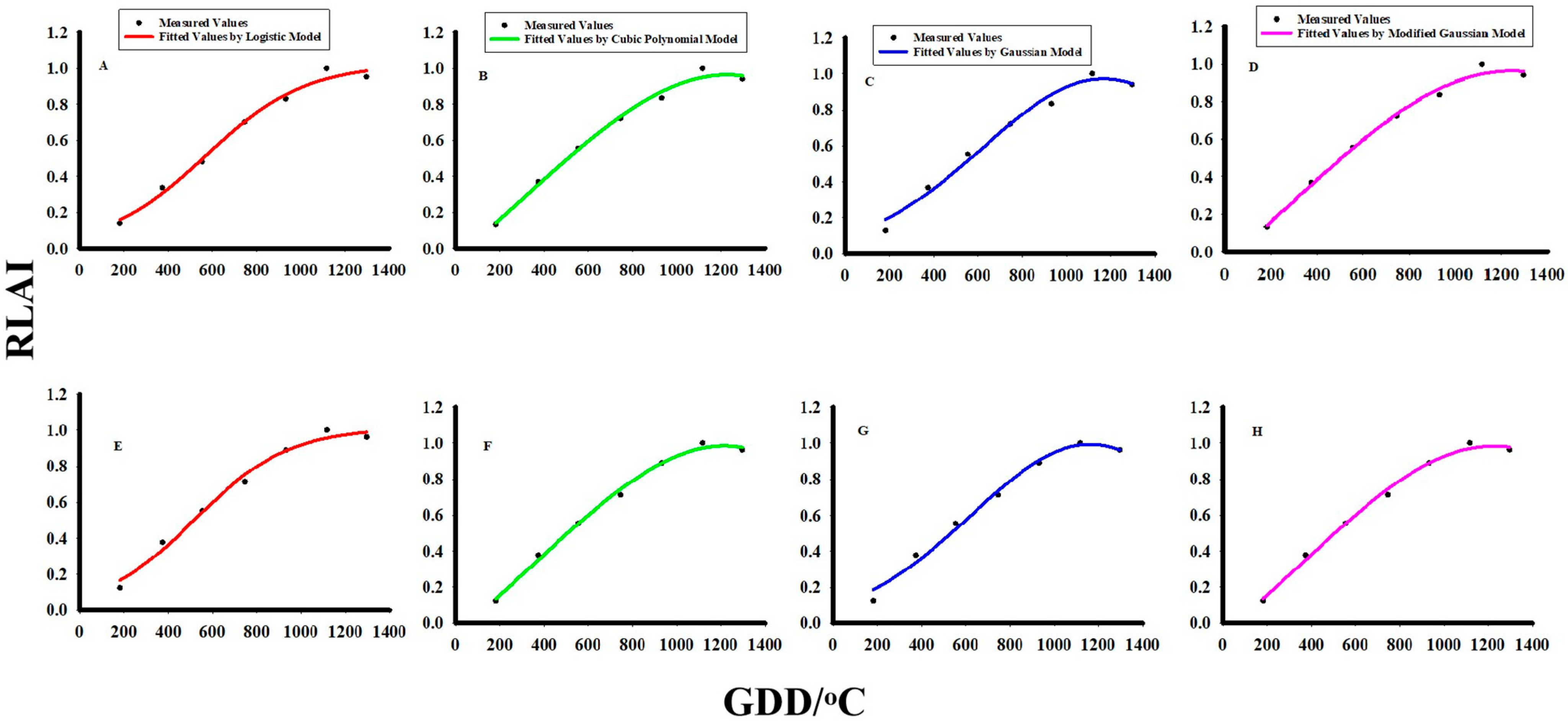
3.1. Simulation of LAI Models Based on GDD

The dynamic changes in the LAI of Hedysarum scoparium over GDD were observed under various treatments of soil amendment and different qualities of water irrigation, as depicted in Figure 2. The LAI values in all soil amendment treatments were taken regularly, in 20-day intervals. In all soil amendment treatments, LAI under saline irrigation was smaller than under fresh water treatment, but these values were mostly non-significant. This indicates that Hedysarum scoparium, as a halophyte plant, showed its ability to maintain growth under stressful conditions [39]. LAI changed among all soil amendment treatments over the whole growing season, while LAI was higher under compost+sandy soil (Figure 2D), manure+sandy soil (Figure 2C), and clay+sandy soil (Figure 2B) as compared with sandy soil (Figure 2A) under different water quality treatments. This indicates that soil amendment materials enhance soil organic matter, increase soil water holding capacity, and reduce infiltration, thereby helping plants sustain their growth under saline conditions and varying temperatures [8,13,40,41]. LAI within all soil amendment treatments under different qualities of irrigation increased rapidly between 200 °C and 1200 °C, then decreased gradually between 1200 °C and 1400 °C, as shown in Figure 2. The maximum LAI was observed when GDD was about 1117.5 °C in all soil amendment treatments under different qualities of irrigation. Based on the results of LAI, GDD holds significant practical importance for the growth of many crops [20]. Researchers globally have extensively investigated crop growth using statistical methods and climate modeling techniques [41,42]. Climate variations have influenced the growth cycle of numerous crops, enhancing their growth. This underscores the significance of climate factors such as GDD in crop growth and development, emphasizing that the role of GDD in modeling studies should not be disregarded [42].

We have developed a straightforward method for normalizing the LAI values to streamline subsequent analyses. Normalization enables us to mitigate the influence of soil amendment treatments, as well as varying water quality treatments, on the dynamic LAI changes in Hedysarum scoparium [43]. Equation (12) was utilized for establishing this relationship.

$$\mathrm{RLAI}={\displaystyle \frac{\mathrm{LAI}}{{\mathrm{LAI}}_{\mathrm{M}}}}$$

(12)

where RLAI is the relative leaf area index.

Table 2. Relative leaf area index values under soil amendment treatments along with different qualities of irrigation water.

Soil Types	GDD	RLAI		Mean RLAI	Standard Deviation
		Fresh Water	Saline Water
Sandy	181.5	0.154	0.165	0.159	0.008
	374	0.475	0.420	0.447	0.038
	554	0.645	0.603	0.624	0.029
	746.5	0.821	0.805	0.813	0.011
	932.5	0.870	0.900	0.885	0.021
	1117.5	1	1	1	0
	1297.5	0.939	0.960	0.949	0.015
Clay+Sandy	181.5	0.132	0.147	0.139	0.010
	374	0.332	0.339	0.336	0.005
	554	0.484	0.479	0.481	0.003
	746.5	0.696	0.707	0.702	0.007
	932.5	0.815	0.845	0.830	0.020
	1117.5	1	1	1	0
	1297.5	0.943	0.961	0.952	0.012
Manure+Sandy	181.5	0.129	0.134	0.132	0.0034
	374	0.392	0.345	0.369	0.033
	554	0.567	0.541	0.554	0.017
	746.5	0.743	0.698	0.721	0.031
	932.5	0.835	0.834	0.835	0.0005
	1117.5	1	1	1	0
	1297.5	0.953	0.927	0.940	0.018
Compost+Sandy	181.5	0.122	0.128	0.126	0.004
	374	0.383	0.373	0.378	0.006
	554	0.574	0.533	0.554	0.029
	746.5	0.729	0.698	0.713	0.02
	932.5	0.897	0.883	0.890	0.0100
	1117.5	1	1	1	0
	1297.5	0.966	0.958	0.962	0.005

Note: GDD = growing degree day, RLAI = relative leaf area index.

shows the RLAI values of all soil amendment treatments under different qualities of irrigation water. The highest RLAI values were obtained in every soil amendment treatment at 1117.5 °C. Overall, the trend of RLAI values was similar in all soil amendment treatments; these results agree with the previous findings [17]. Consequently, mathematical RLAI models were developed using the mean RLAI values from all soil treatments and water treatments.

The mean RLAI values for different soil amendment treatments were fitted using various growth models. A genetic algorithm was employed to optimize the parameters of these models, and the resultant fitted models are illustrated in Figure 3 and Figure 4. These fitted models demonstrate good agreement with the observed RLAI values, particularly the late stable period and period of decline. Across all these fitted models, the correlation between observed and predicted values falls within 0.97 to 0.99.

Table 3. Fitted values on the mathematical growth models along with error values.

Soil Types	Expression	RE %	RMSE	R2
Sandy
Logistic model	$\mathrm{RLAI}={\displaystyle \frac{1.13}{1+{\mathrm{e}}^{-.\left(\frac{\mathrm{GDD}-473.44}{330.24}\right)}}}$	4.6	0.0054	0.99
Gaussian model	$\mathrm{RLAI}=0.99·{\mathrm{e}}^{\left[-0.5·{\left({\displaystyle \frac{\mathrm{GDD}-1112}{550.34}}\right)}^2\right]}$	4.2	0.0037	0.97
Modified Gaussian model	$\mathrm{RLAI}=1.001·{\mathrm{e}}^{\left[-0.5·{\left({\displaystyle \frac{\left|\mathrm{GDD}-1280.4\right|}{287.90}}\right)}^{0.75}\right]}$	3.3	0.0025	0.99
Cubic model	$\begin{array}{c}\mathrm{RLAI}=0.06+2.23\times {10}^{-4}\times \mathrm{GDD}-1.46\times {10}^{-7}\times {\mathrm{GDD}}^2\\ -8.5\times {10}^{-10}\times {\mathrm{GDD}}^3\end{array}$	3.7	0.0032	0.99
Clay+Sandy
Logistic model	$\mathrm{RLAI}={\displaystyle \frac{1.02}{1+{\mathrm{e}}^{-.\left(\frac{\mathrm{GDD}-569.55}{227.42}\right)}}}$	4.4	0.0075	0.99
Gaussian model	$\mathrm{RLAI}=0.97·{\mathrm{e}}^{\left[-0.5·{\left({\displaystyle \frac{\mathrm{GDD}-1197.50}{541.17}}\right)}^2\right]}$	3.1	0.0055	0.99
Modified Gaussian model	$\mathrm{RLAI}=0.90$$.{\mathrm{e}}^{\left[-0.5·{\left({\displaystyle \frac{\left|\mathrm{GDD}-1184.56\right|}{521.07}}\right)}^{1.9}\right]}$	1.5	0.0043	0.99
Cubic model	$\begin{array}{c}\mathrm{RLAI}=-0.122+1.68\times {10}^{-3}\times \mathrm{GDD}-5\times {10}^{-7}\times {\mathrm{GDD}}^2\\ -1.16\times {10}^{-10}\times {\mathrm{GDD}}^3\end{array}$	1.9	0.0049	0.99
Manure+Sandy
Logistic model	$\mathrm{RLAI}={\displaystyle \frac{1.03}{1+{\mathrm{e}}^{-.\left(\frac{\mathrm{GDD}-564.45}{232.42}\right)}}}$	3.5	0.062	0.98
Gaussian model	$\mathrm{RLAI}=0.97·{\mathrm{e}}^{\left[-0.5·{\left({\displaystyle \frac{\mathrm{GDD}-1168.20}{547.22}}\right)}^2\right]}$	2.1	0.057	0.98
Modified Gaussian model	$\mathrm{R}\mathrm{LAI}=1.70·{\mathrm{e}}^{\left[-0.5·{\left({\displaystyle \frac{\left|\mathrm{GDD}-1246.72\right|}{927.48}}\right)}^{-0.74}\right]}$	1.5	0.032	0.99
Cubic model	$\begin{array}{c}\mathrm{RLAI}=-0.04+9.01\times {10}^{-4}\times \mathrm{GDD}-4.16\times {10}^{-7}\times {\mathrm{GDD}}^2\\ -4.4\times {10}^{-10}\times {\mathrm{GDD}}^3\end{array}$	1.9	0.047	0.99
Compost+Sandy
Logistic model	$\mathrm{RLAI}={\displaystyle \frac{1.01}{1+{\mathrm{e}}^{-.\left(\frac{\mathrm{GDD}-522.02}{211.11}\right)}}}$	2.9	0.085	0.98
Gaussian model	$\mathrm{RLAI}=0.99·{\mathrm{e}}^{\left[-0.5·{\left({\displaystyle \frac{\mathrm{GDD}-1162.69}{537.28}}\right)}^2\right]}$	2.1	0.071	0.98
Modified Gaussian model	$\mathrm{R}\mathrm{LAI}=1.56·{\mathrm{e}}^{\left[-0.5·{\left({\displaystyle \frac{\left|\mathrm{GDD}-1228.59\right|}{882.35}}\right)}^{-0.58}\right]}$	1.3	0.051	0.99
Cubic model	$\begin{array}{c}\mathrm{RLAI}=-0.04+9.22\times {10}^{-4}\times \mathrm{GDD}+5.73\times {10}^{-7}\times {\mathrm{GDD}}^2\\ -5.22\times {10}^{-10}\times {\mathrm{GDD}}^3\end{array}$	1.7	0.058	0.99

Note: RMSE = root mean square error, R² = coefficient of determination, Re = relative error.

shows the fitted results of the experience parameters across the four models. Across all models, the coefficient of determination exceeds 0.97, and relative errors are below 5%. This indicates a strong alignment between the predicted results and the measured data across all soil amendment treatments, especially during the later growth phases [25,34]. The fitted results of this present study also agreed with the findings of cotton, grapes, sesbania, and cluster bean [15,20,25]. Among all models, the modified Gaussian model and Cubic polynomial model demonstrate superior accuracy compared to the other models. Cubic polynomial models are more suitable among all developed models due to their simple quadratic equations that can be solved by using their first derivative [44]. While the Cubic polynomial model is not able to explain the complex relationship between growth parameters [23], under these conditions, the modified Gaussian model is best under all soil amendment treatments.

Gaussian and modified Gaussian models containing exponential functions. The parameter GDD₀ in the models represents the growing degree days at the maximum relative leaf area index (RLAI_max = 1). The deviation between the values of LAI_M in these two models under sandy soil treatment 0.99 and 0.001 and clay+sandy soil treatment is 0.98 and 0.90. Similarly, the manure+sandy soil treatment values are 0.97 and 0.70, and the compost+sandy soil treatment values are 0.99 and 0.56, respectively. It can be said, according to the results, that the predicted LAI_M values are smaller than the measured values by using a modified Gaussian model. When using the Gaussian model, predicted LAI_M values are larger than measured values. However, it is important to note that the absolute deviation of LAI_M can serve as a measure of predictive accuracy, and in this regard, the modified Gaussian model outperforms the others, demonstrating the highest level of performance [20,23].

The number of parameters is highly sensitive and related to model flexibility and applicability [35]. An increased number of parameters can increase the applicability of the model, but the accuracy of the model decreased [45]. As shown in Table 3, the Cubic polynomial model and modified Gaussian model have four parameters, but the Logistic model and Gaussian model have only three parameters. It should be noted that a higher number of parameters makes results more complex [46]. Therefore, in situations where higher precision is not imperative, it is advisable to utilize Gaussian and Logistic growth models for predicting LAI of Hedysarum scoparium [47].

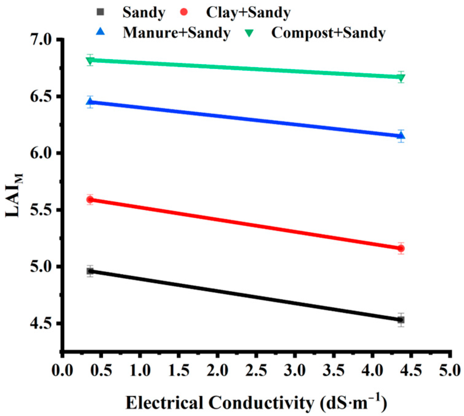
3.2. Relationship between Leaf Area Index and Water Quality under Soil Amendment Treatments

The maximum leaf area index (LAI_M) is an important parameter when predicting LAI. Equations (5)–(8) describe the maximum leaf area index. Therefore, the value of these models depends on their ability to calculate LAI_M quickly and easily [48]. However, it is crucial to acknowledge that the LAI is influenced by various factors such as temperature [49], soil conditions [50], GDD [4], irrigation practices [51], and water usage. In field experiments, certain parameters pose challenges for regular measurement. Therefore, the capability to estimate LAI using readily available data is crucial for enhancing the practical utility of the method in day-to-day operations. In this study, LAI_M can be directly measured for Hedysarum scoparium plants when the GDD reaches 1117.5 °C across various soil amendment treatments and water quality conditions, as illustrated in Table 2. Additionally, saline water irrigation affects the growth of halophyte plants in their early growth stages. For this purpose, soil amendments help plants to sustain their growth under saline and high-temperature conditions [14,52]. Therefore, in this study, soil amendments play a significant role in the development of plant growth under saline conditions. The relationship between different water quality treatments and LAI_M under different soil amendments can be determined using the data from this study, as shown in Figure 5.

It is very much clear by the expression that soil amendments take part in overcoming the saline water irrigation effects on the growth of Hedysarum scoparium plants. From Figure 5, we can observe a significant increase in LAI_M in soil amendment treatments compared to sandy soil. Only two water treatments were used in this study, so the relationship between LAI_M and water quality can be determined with a linear equation in all soil amendment treatments.

$${\mathrm{LAI}}_{\mathrm{M}}=4.99-0.107\times \mathrm{EC}$$

(13)

$${\mathrm{LAI}}_{\mathrm{M}}=5.62-0.107\times \mathrm{EC}$$

(14)

$${\mathrm{LAI}}_{\mathrm{M}}=6.47-0.07\times \mathrm{EC}$$

(15)

$${\mathrm{LAI}}_{\mathrm{M}}=6.83-0.03\times \mathrm{EC}$$

(16)

Equations (13) and (14) explain the relationship between sandy soil and clay+sandy soil. Furthermore, Equations (15) and (16) explain the relationship between manure+sandy soil and compost+sandy soil. EC is the electrical conductivity of water. The coefficient of determination in all four equations is 0.99.

Let

$${\mathrm{LAI}}_{\mathrm{M}}=0$$

Then, the EC values of Equations (13)–(16) become:

$$\mathrm{EC}=46.63 \mathrm{dS}·{\mathrm{m}}^{-1}$$

(17)

$$\mathrm{EC}=52.62 \mathrm{dS}·{\mathrm{m}}^{-1}$$

(18)

$$\mathrm{EC}=92.42 \mathrm{dS}·{\mathrm{m}}^{-1}$$

(19)

$$\mathrm{EC}=227.66 \mathrm{dS}·{\mathrm{m}}^{-1}$$

(20)

Equations (17)–(20) show that soil amendments help the plant increase its salt tolerance [53].

If we manipulate Equations (12)–(16), then the leaf area index relationship for electrical conductivity and relative leaf area index for all soil amendments are described below in Equation (21) for sandy soil and (22) for clay+sandy. Similarly, Equations (23) and (24) represent those for manure+sandy and compost+sandy soil, respectively.

$$\mathrm{LAI}= \mathrm{RLAI} \ast (4.99-0.107\times \mathrm{EC})$$

(21)

$$\mathrm{LAI}=\mathrm{RLAI} \ast \left(5.62-0.107\times \mathrm{EC}\right)$$

(22)

$$\mathrm{LAI}=\mathrm{RLAI} \ast \left(6.47-0.07\times \mathrm{EC}\right)$$

(23)

$$\mathrm{LAI}=\mathrm{RLAI} \ast \left(6.83-0.03\times \mathrm{EC}\right)$$

(24)

These LAI relationship findings agree with the findings of previous work [20,23,25]. Manipulating the models in Table 2 with Equations (21)–(24), the mathematical prediction model for LAI in all soil amendment treatments can be established. Therefore, the Logistic model for LAI in all soil amendments is given below:

$$\mathrm{LAI}={\displaystyle \frac{1.13}{1+{\mathrm{e}}^{-.\left(\frac{\mathrm{GDD}-473.44}{330.24}\right)}}}\ast (4.99-0.107\times \mathrm{EC})$$

(25)

$$\mathrm{LAI}={\displaystyle \frac{1.02}{1+{\mathrm{e}}^{-.\left(\frac{\mathrm{GDD}-569.55}{227.42}\right)}}}\ast \left(5.62-0.107\times \mathrm{EC}\right)$$

(26)

$$\mathrm{LAI}={\displaystyle \frac{1.03}{1+{\mathrm{e}}^{-.\left(\frac{\mathrm{GDD}-564.45}{232.42}\right)}}}\ast \left(6.47-0.07\times \mathrm{EC}\right)$$

(27)

$$\mathrm{LAI}={\displaystyle \frac{1.01}{1+{\mathrm{e}}^{-.\left(\frac{\mathrm{GDD}-522.02}{211.11}\right)}}}\ast \left(6.83-0.03\times \mathrm{EC}\right)$$

(28)

Equations (25) and (26) explain the relationship between LAI, GDD, and different qualities of irrigation for sandy soil and clay+sandy soil. Furthermore, Equations (27) and (28) explain the relationship between LAI, GDD, and different qualities of irrigation for manure+sandy soil and compost+sandy soil. Figure 6 depicts the fitted results between measured and predicted values for the mathematical models, which exhibit the same trends as found in previous analyses [15]. The fitted results of RLAI within different soil amendments under different qualities of irrigation are shown in Table 3.

Figure 6 shows the fitted results between measured and predicted values of all models under different soil amendment treatments along with different qualities of irrigation. The R² values in all soil amendment treatments are between 0.98 and 0.99. RMSE values and relative error (Re) values in all soil amendment treatments are below 1%. Modified Gaussian and Logistic models should be considered for calculating the leaf area index under different soil amendments in saline irrigation. These findings are consistent with previous research [17,23,29].

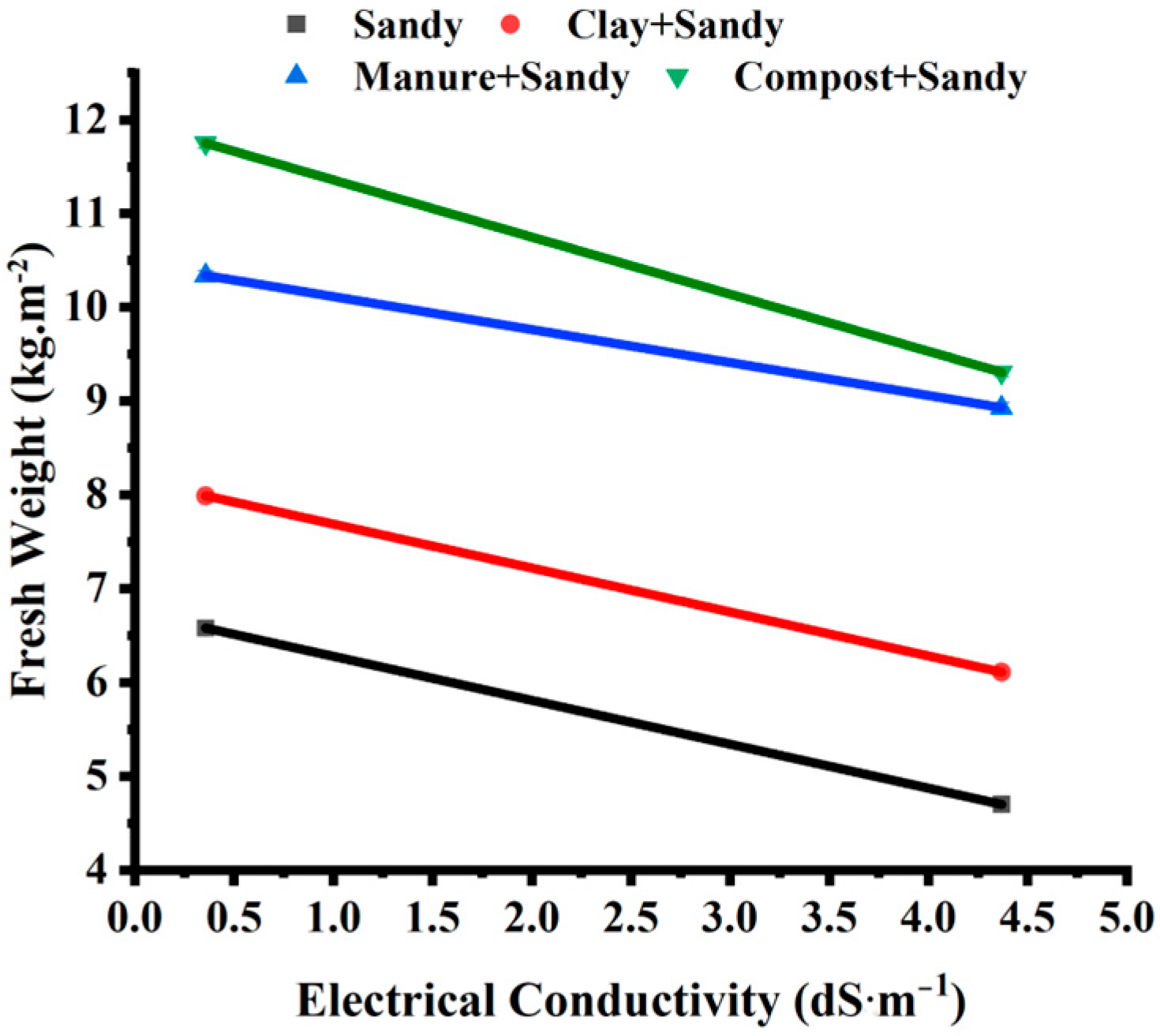
3.3. Mathematical Models for Biomass Production under Soil Amendments

Simulation data indicate a direct correlation between crop water productivity and plant biomass, with transpiration levels playing a crucial role. Crop water relationship or productivity can be estimated per unit of water transpired per plant biomass per unit area, i.e., g·m⁻², kg·ha⁻¹ [44]. The relationship between water productivity and plant biomass is mostly linear [45]. Figure 7 describes the relationship between plant biomass across different water quality treatments under various soil amendments.

The relationship between plant biomass (kg·m⁻²) under different qualities of water is linear because saline water creates a negative effect on plant growth.

$$\mathrm{B}=6.74-0.46\times \mathrm{EC}$$

(29)

$$\mathrm{B}=8.15-0.46\times \mathrm{EC}$$

(30)

$$\mathrm{B}=10.46-0.35\times \mathrm{EC}$$

(31)

$$\mathrm{B}=11.96-0.6\times \mathrm{EC}$$

(32)

where B indicates plant biomass production. Equations (29) and (30) explain the relationship between plant biomass and water quality irrigation for sandy soil and clay+sandy soil. Furthermore, Equations (31) and (32) explain the relationship for manure+sandy soil and compost+sandy soil.

If we manipulate Equations (25)–(32), the new equations are as follows:

$$\mathrm{B}=6.74-0.46\ast \{{\displaystyle \frac{1}{0.107}}\ast ({\displaystyle \frac{1.13}{1+{\mathrm{e}}^{-.\left(\frac{\mathrm{GDD}-473.44}{330.24}\right)}}}\ast 4.99-\mathrm{LAI})\}$$

(33)

$$\mathrm{B}=8.15-0.46\ast \{{\displaystyle \frac{1}{0.107}}\ast ({\displaystyle \frac{1.02}{1+{\mathrm{e}}^{-.\left(\frac{\mathrm{GDD}-569.55}{227.42}\right)}}}\ast 5.62-\mathrm{LAI})\}$$

(34)

$$\mathrm{B}=10.46-0.35\ast \{{\displaystyle \frac{1}{0.07}}\ast ({\displaystyle \frac{1.03}{1+{\mathrm{e}}^{-.\left(\frac{\mathrm{GDD}-564.45}{232.42}\right)}}}\ast 6.47-\mathrm{LAI})\}$$

(35)

$$\mathrm{B}=11.96-0.6\ast \{{\displaystyle \frac{1}{0.03}}\ast ({\displaystyle \frac{1.01}{1+{\mathrm{e}}^{-.\left(\frac{\mathrm{GDD}-522.02}{211.11}\right)}}}\ast 6.83-\mathrm{LAI})\}$$

(36)

Equations (33) and (34) explain the relationship between plant biomass, LAI, and GDD for sandy soil and clay+sandy soil by using the Logistic model. Furthermore, Equations (35) and (36) explain the relationship between plant biomass, LAI, and GDD for manure+sandy soil and compost+sandy soil by using the Logistic model. Relationships with other models between plant biomass, LAI, and GDD can be developed by using the same steps. GDD has a great influence on the growth of LAI, plant height, biomass production, and harvest index [54]. On the other hand, LAI has a significant influence on biomass production per plant. Therefore, in modeling studies, the effects of these parameters must not be ignored [55]. LAI is a critical factor in various models, such as evapotranspiration and canopy photosynthesis [56]. It plays a key role in the plant–atmosphere relationship by transferring energy and mass between the canopy and atmosphere [57]. In short, models developed with the help of LAI and GDD have a great impact on the prediction of biomass and other parameters. According to Figure 6, the modified Gaussian model and Cubic polynomial model are best for predicting LAI. Therefore, we can assume a similar trend will be found for biomass production, as these relationships were developed based on the interpretation of these equations.

4. Conclusions

In arid regions, fresh water scarcity, temperature variations, and poor nutrients in the soil always create negative effects on crop growth. In this study, we analyzed the response of LAI to climatic variables such as GDD under different qualities of irrigation along with various soil amendment treatments. The results indicate that LAI is mainly affected by GDD and saline water irrigation. The main conclusions of this study are given below:

(a)

Soil amendments like manure+sandy soil and compost+sandy soil boost the growth of Hedysarum scoparium under saline water irrigation compared with sandy soil.

(b)

Mathematical models between LAI and different water qualities of irrigation have been developed under different soil amendment treatments.

(c)

The relationship between RLAI and GDD has been developed under different soil amendment treatments.

(d)

Mathematical models between plant biomass production, GDD, and LAI have been developed under different water qualities of irrigation along with various soil amendment treatments.

It was concluded that these predicted mathematical models can provide crucial insights for enhancing production in arid regions. By using eco-friendly soil amendments, they improve water use efficiency across diverse irrigation water qualities.

References

1. Azeem, A.; Javed, Q.; Sun, J.; Nawaz, M.I.; Ullah, I.; Kama, R.; Du, D. Functional traits of okra cultivars (Chinese green and Chinese red) under salt stress. Folia Hortic. 2020, 32, 159–170. [Google Scholar] [CrossRef]
2. Che, Z.; Wang, J.; Li, J. Effects of water quality, irrigation amount and nitrogen applied on soil salinity and cotton production under mulched drip irrigation in arid Northwest China. Agric. Water Manag. 2021, 247, 106738. [Google Scholar] [CrossRef]
3. Ma, K.; Wang, Z.; Li, H.; Wang, T.; Chen, R. Effects of nitrogen application and brackish water irrigation on yield and quality of cotton. Agric. Water Manag. 2022, 264, 107512. [Google Scholar] [CrossRef]
4. Chen, Y.; Wang, L.; Bai, Y.L.; Lu, Y.L.; Ni, L.; Wang, Y.H.; Xu, M.Z. Quantitative relationship between effective accumulated temperature and plant height & leaf area index of summer maize under different nitrogen, phosphorus and potassium levels. Sci. Agric. Sin. 2021, 54, 4761–4777. [Google Scholar]
5. Liu, B.; Wang, S.; Kong, X.; Liu, X.; Sun, H. Modeling and assessing feasibility of long-term brackish water irrigation in vertically homogeneous and heterogeneous cultivated lowland in the North China Plain. Agric. Water Manag. 2019, 211, 98–110. [Google Scholar] [CrossRef]
6. Zhu, M.; Wang, Q.; Sun, Y.; Zhang, J. Effects of oxygenated brackish water on germination and growth characteristics of wheat. Agric. Water Manag. 2021, 245, 106520. [Google Scholar] [CrossRef]
7. He, P.; Yu, S.; Zhang, F.; Ma, T.; Ding, J.; Chen, K.; Chen, X.; Dai, Y. Effects of soil water regulation on the cotton yield, fiber quality and soil salt accumulation under mulched drip irrigation in southern Xinjiang, China. Agronomy 2022, 12, 1246. [Google Scholar] [CrossRef]
8. Guarnieri, S.F.; Nascimento, E.C.D.; Costa, R.F.; Faria, J.L.B.D.; Lobo, F.D.A. Coconut fiber biochar alters physical and chemical properties in sandy soils. Acta Sci. Agron. 2021, 43, e51801. [Google Scholar] [CrossRef]
9. Zhang, T.; Fan, J.; Wang, S.; Xu, X.; Chai, Z. Photosynthetic characteristics of Haloxylon ammodendron under high salinity water irrigation. J. Desert Res. 2020, 40, 112. [Google Scholar]
10. Guo, Y.; Wang, Q.; Zhao, X.; Li, Z.; Li, M.; Zhang, J.; Wei, K. Field irrigation using magnetized brackish water affects the growth and water consumption of Haloxylon ammodendron seedlings in an arid area. Front. Plant Sci. 2022, 13, 929021. [Google Scholar] [CrossRef]
11. Feizi, Z.; Ayoubi, S.; Mosaddeghi, M.R.; Besalatpour, A.A.; Zeraatpisheh, M.; Rodrigo-Comino, J. A wind tunnel experiment to investigate the effect of polyvinyl acetate, biochar, and bentonite on wind erosion control. Arch. Agron. Soil Sci. 2019, 65, 1049–1062. [Google Scholar] [CrossRef]
12. Asl, F.N.; Asgari, H.R.; Emami, H.; Jafari, M. Combined effect of micro silica with clay, and gypsum as mulches on shear strength and wind erosion rate of sands. Int. Soil Water Conserv. Res. 2019, 7, 388–394. [Google Scholar]
13. Mi, J.; Gregorich, E.G.; Xu, S.; McLaughlin, N.B.; Liu, J.; Zhao, B. Bentonite effects on soil physical properties and millet yield components in a semi-arid region in China. Can. J. Soil Sci. 2021, 101, 749–760. [Google Scholar] [CrossRef]
14. Mi, J.; Gregorich, E.G.; Xu, S.; McLaughlin, N.B.; Ma, B.; Liu, J. Changes in soil biochemical properties following application of bentonite as a soil amendment. Eur. J. Soil Biol. 2021, 102, 103251. [Google Scholar] [CrossRef]
15. Su, L.; Tao, W.; Sun, Y.; Shan, Y.; Wang, Q. Mathematical models of leaf area index and yield for grapevines grown in the turpan area, xinjiang, China. Agronomy 2022, 12, 988. [Google Scholar] [CrossRef]
16. Wang, K.; Su, L.; Wang, Q. Cotton growth model under drip irrigation with film mulching: A case study of Xinjiang, China. Agron. J. 2021, 113, 2417–2436. [Google Scholar] [CrossRef]
17. Su, L.; Wang, Q.; Wang, C.; Shan, Y. Simulation models of leaf area index and yield for cotton grown with different soil conditioners. PLoS ONE 2015, 10, e0141835. [Google Scholar] [CrossRef] [PubMed]
18. Liben, F.; Wortmann, C.; Yang, H.; Lindquist, J.; Tadesse, T.; Wegary, D. Crop model and weather data generation evaluation for conservation agriculture in Ethiopia. Field Crops Res. 2018, 228, 122–134. [Google Scholar] [CrossRef]
19. Manivasagam, V.; Rozenstein, O. Practices for upscaling crop simulation models from field scale to large regions. Comput. Electron. Agric. 2020, 175, 105554. [Google Scholar] [CrossRef]
20. Azeem, A.; Mai, W.; Ali, R. Modeling Plant Height and Biomass Production of Cluster Bean and Sesbania across Diverse Irrigation Qualities in Pakistan’s Thar Desert. Water 2024, 16, 9. [Google Scholar] [CrossRef]
21. Liu, J.-H.; Yan, Y.; Ali, A.; Yu, M.-F.; Xu, Q.-J.; Shi, P.-J.; Chen, L. Simulation of crop growth, time to maturity and yield by an improved sigmoidal model. Sci. Rep. 2018, 8, 7030. [Google Scholar] [CrossRef] [PubMed]
22. Wang, H.; Sánchez-Molina, J.; Li, M.; Berenguel, M.; Yang, X.; Bienvenido, J. Leaf area index estimation for a greenhouse transpiration model using external climate conditions based on genetics algorithms, back-propagation neural networks and nonlinear autoregressive exogenous models. Agric. Water Manag. 2017, 183, 107–115. [Google Scholar] [CrossRef]
23. Chianucci, F.; Cutini, A.; Corona, P.; Puletti, N. Estimation of leaf area index in understory deciduous trees using digital photography. Agric. For. Meteorol. 2014, 198, 259–264. [Google Scholar] [CrossRef]
24. Liu, Y.; Su, L.; Wang, Q.; Zhang, J.; Shan, Y.; Deng, M. Comprehensive and quantitative analysis of growth characteristics of winter wheat in China based on growing degree days. Adv. Agron. 2020, 159, 237–273. [Google Scholar]
25. Wang, Q.J.; Lin, S.D.; Su, L.J. Quantitative analysis of response of potato main growth index to growing degree days. Trans. Chin. Soc. Agric. Mach 2020, 51, 306–316. [Google Scholar]
26. Liu, F.; Liu, Y.; Su, L.; Tao, W.; Wang, Q.; Deng, M. Integrated growth model of typical crops in China with regional parameters. Water 2022, 14, 1139. [Google Scholar] [CrossRef]
27. Su, L.; Liu, Y.; Wang, Q. Rice growth model in China based on growing degree days. Trans. Chin. Soc. Agric. Eng 2020, 36, 162–174. [Google Scholar]
28. Setiyono, T.; Weiss, A.; Specht, J.E.; Cassman, K.G.; Dobermann, A. Leaf area index simulation in soybean grown under near-optimal conditions. Field Crops Res. 2008, 108, 82–92. [Google Scholar] [CrossRef]
29. Wang, Q.; Wang, K.; Su, L.; Zhang, J.; Wei, K. Effect of irrigation amount, nitrogen application rate and planting density on cotton leaf area index and yield. Trans. Chin. Soc. Agric. Mach 2021, 52, 300–312. [Google Scholar]
30. Xue, J.; Wang, X.; Du, X.; Mao, P.; Zhang, T.; Zhao, L.; Han, J. Influence of salinity and temperature on the germination of Hedysarum scoparium Fisch. et Mey. Afr. J. Biotechnol. 2012, 11, 3244–3249. [Google Scholar]
31. Ma, J.; Wang, H.; Jin, L.; Zhang, P. Comparative analysis of physiological responses to environmental stress in Hedysarum scoparium and Caragana korshinskii seedlings due to roots exposure. PeerJ 2023, 11, e14905. [Google Scholar] [CrossRef] [PubMed]
32. Zhou, Z.; Yu, M.; Ding, G.; Gao, G.; He, Y.; Wang, G. Effects of Hedysarum leguminous plants on soil bacterial communities in the Mu Us Desert, northwest China. Ecol. Evol. 2020, 10, 11423–11439. [Google Scholar] [CrossRef] [PubMed]
33. Mai, W.; Xue, X.; Azeem, A. Growth of cotton crop (Gossypium hirsutum L.) higher under drip irrigation because of better phosphorus uptake. Appl. Ecol. Environ. Res. 2022, 20, 4865–4878. [Google Scholar] [CrossRef]
34. Azeem, A.; Mai, W.; Tian, C.; Javed, Q. Dry Weight Prediction of Wedelia trilobata and Wedelia chinensis by Using Artificial Neural Network and MultipleLinear Regression Models. Water 2023, 15, 1896. [Google Scholar] [CrossRef]
35. Mai, W.; Xue, X.; Azeem, A. Plant Density Differentially Influences Seed Weight in Different Portions of the Raceme of Castor. Pol. J. Environ. Stud. 2023, 32, 3247–3254. [Google Scholar] [CrossRef]
36. McMaster, G.S.; Wilhelm, W. Growing degree-days: One equation, two interpretations. Agric. For. Meteorol. 1997, 87, 291–300. [Google Scholar] [CrossRef]
37. Yang, L.; Wang, Y.; Kang, M.; Dong, Q. Simulation of tomato fruit individual growth rule based on revised logistic model. Trans. Chin. Soc. Agric. Mach. 2008, 39, 81–84. [Google Scholar]
38. Wang, R.; Li, S.; Wang, Q.; Zheng, J.; Fan, J.; Li, S. Evaluation of simulation models of spring-maize leaf area and biomass in semiarid agro-ecosystems. Chin. J. Eco-Agric. 2008, 16, 139–144. [Google Scholar] [CrossRef]
39. Wei, C.; Ren, S.; Xu, Z.; Zhang, M.; Wei, R.; Yang, P. Effects of irrigation water salinity and irrigation water amount on greenhouse gas emissions and spring maize growth. Trans. Chin. Soc. Agric. Mach. 2021, 52, 251–260. [Google Scholar]
40. Younas, T.; Cabello, G.; Taype, M.; Cardenas, J.; Trujillo, P.; Salas-Contreras, W.; Yaulilahua-Huacho, R.; Areche, F.; Rodriguez, A.; Nieto, D.C. Conditioning of desert sandy soil and investigation of the ameliorative effects of poultry manure and bentonite treatment rate on plant growth. Braz. J. Biol. 2023, 82, e269137. [Google Scholar] [CrossRef] [PubMed]
41. Arora, A.; Nandal, P.; Chaudhary, A. Critical evaluation of novel applications of aquatic weed Azolla as a sustainable feedstock for deriving bioenergy and feed supplement. Environ. Rev. 2022, 31, 195–205. [Google Scholar] [CrossRef]
42. Vanuytrecht, E.; Raes, D.; Steduto, P.; Hsiao, T.C.; Fereres, E.; Heng, L.K.; Vila, M.G.; Moreno, P.M. AquaCrop: FAO’s crop water productivity and yield response model. Environ. Model. Softw. 2014, 62, 351–360. [Google Scholar] [CrossRef]
43. Wypych, A.; Sulikowska, A.; Ustrnul, Z.; Czekierda, D. Variability of growing degree days in Poland in response to ongoing climate changes in Europe. Int. J. Biometeorol. 2017, 61, 49–59. [Google Scholar] [CrossRef] [PubMed]
44. Cardei, P.; Nenciu, F.; Ungureanu, N.; Pruteanu, M.A.; Vlăduț, V.; Cujbescu, D.; Găgeanu, I.; Cristea, O.D. Using Statistical Modeling for Assessing Lettuce Crops Contaminated with Zn, Correlating Plants Growth Characteristics with the Soil Contamination Levels. Appl. Sci. 2021, 11, 8261. [Google Scholar] [CrossRef]
45. Azeem, A.; Javed, Q.; Sun, J.; Du, D. Artificial neural networking to estimate the leaf area for invasive plant Wedelia trilobata. Nord. J. Bot. 2020, 38. [Google Scholar] [CrossRef]
46. Azeem, A.; Wenxuan, M.; Changyan, T.; Qamar, M.U.; Buttar, N.A. Prediction of Wedelia trilobata Growth under Flooding and Nitrogen Enrichment Conditions by Using Artificial Neural Network Model. Pol. J. Environ. Stud. 2024, 33, 1007–1015. [Google Scholar] [CrossRef]
47. Javed, Q.; Azeem, A.; Sun, J.; Ullah, I.; Du, D.; Imran, M.A.; Nawaz, M.I.; Chattha, H.T. Growth prediction of Alternanthera philoxeroides under salt stress by application of artificial neural networking. Plant Biosyst.-Int. J. Deal. All Asp. Plant Biol. 2022, 156, 61–67. [Google Scholar]
48. Li, L.; Chen, S.; Yang, C.; Meng, F.; Sigrimis, N. Prediction of plant transpiration from environmental parameters and relative leaf area index using the random forest regression algorithm. J. Clean. Prod. 2020, 261, 121136. [Google Scholar] [CrossRef]
49. Yadav, S.; Modi, P.; Dave, A.; Vijapura, A.; Patel, D.; Patel, M. Effect of abiotic stress on crops. Sustain. Crop Prod. 2020, 3, 5–16. [Google Scholar]
50. Garbowski, T.; Bar-Michalczyk, D.; Charazińska, S.; Grabowska-Polanowska, B.; Kowalczyk, A.; Lochyński, P. An overview of natural soil amendments in agriculture. Soil Tillage Res. 2023, 225, 105462. [Google Scholar] [CrossRef]
51. Hailu, B.; Mehari, H. Impacts of soil salinity/sodicity on soil-water relations and plant growth in dry land areas: A review. J. Nat. Sci. Res 2021, 12, 1–10. [Google Scholar]
52. Adhikari, S.; Timms, W.; Mahmud, M.P. Optimising water holding capacity and hydrophobicity of biochar for soil amendment–A review. Sci. Total Environ. 2022, 851, 158043. [Google Scholar] [CrossRef] [PubMed]
53. Azeem, A.; Sun, J.; Javed, Q.; Jabran, K.; Du, D. The effect of submergence and eutrophication on the trait’s performance of Wedelia trilobata over its congener native Wedelia chinensis. Water 2020, 12, 934. [Google Scholar] [CrossRef]
54. Liu, L.-W.; Lu, C.-T.; Wang, Y.-M.; Lin, K.-H.; Ma, X.; Lin, W.-S. Rice (Oryza sativa L.) growth modeling based on growth degree day (GDD) and artificial intelligence algorithms. Agriculture 2022, 12, 59. [Google Scholar] [CrossRef]
55. Ghamghami, M.; Ghahreman, N.; Irannejad, P.; Ghorbani, K. Comparison of data mining and GDD-based models in discrimination of maize phenology. Int. J. Plant Prod. 2019, 13, 11–22. [Google Scholar] [CrossRef]
56. Azeem, A.; Wenxuan, M.; Ali, R.; Abbas, A.; Hussain, N.; Kazmi, A.H.; Butt, U.A. Evaluating salt tolerance in fodder crops: A field experiment in the dry land. Open Agric. 2024, 9, 20220307. [Google Scholar] [CrossRef]
57. Davoodi, E.; Ghasemieh, H.; Batelaan, O.; Abdollahi, K. Spatial-temporal simulation of LAI on basis of rainfall and growing degree days. Remote Sens. 2017, 9, 1207. [Google Scholar] [CrossRef]
Figure 1. (A) Experimental design with treatments details and (B) experimental site. Note: SECME means Sindh Engro Coal Mining Company. Non-English words means Jamia Mosque.
Resources 13 00110 g001
Figure 2. Changes in leaf area index over growing degree days (GDDs) under different soil amendments and different water quality treatments. (A) represents sandy soil, (B) represents clay+sandy soil, (C) represents manure+sandy soil, and (D) represents compost+sandy soil.
Resources 13 00110 g002
Figure 3. Comparison between measured and predicted values of relative leaf area index (RLAI). (A) represents Logistic model under sandy soil, (B) represents Cubic polynomial model under sandy soil, (C) represents Gaussian model under sandy soil, and (D) represents modified Gaussian model under sandy soil. Similarly, (E) represents Logistic model under clay+sandy soil, (F) represents Cubic polynomial model under clay+sandy soil, (G) represents Gaussian model under clay+sandy soil, and (H) represents modified Gaussian model under clay+sandy soil.
Resources 13 00110 g003
Figure 4. Comparison between measured and predicted values of relative leaf area index (RLAI). (A) represents Logistic model under manure+sandy soil, (B) represents Cubic polynomial model under manure+sandy soil, (C) represents Gaussian model under manure+sandy soil, and (D) represents modified Gaussian model under manure+sandy soil. Similarly, (E) represents Logistic model under compost+sandy soil, (F) represents Cubic polynomial model under compost+sandy soil, (G) represents Gaussian model under compost+sandy soil, and (H) represents modified Gaussian model under compost+sandy soil.
Resources 13 00110 g004
Figure 5. Relationship between maximum leaf area index and water quality treatments under different soil amendments. Note: LAIM = maximum leaf area index.
Resources 13 00110 g005
Figure 6. Measured and predicted values of relative leaf area index by using models in Table 2. (A) represents Logistic model under sandy soil, (B) represents Cubic polynomial model under sandy soil, (C) represents Gaussian model under sandy soil, and (D) represents modified Gaussian model under sandy soil. (E) represents Logistic model under clay+sandy soil, (F) represents Cubic polynomial model under clay+sandy soil, (G) represents Gaussian model under clay+sandy soil, and (H) represents modified Gaussian model under clay+sandy soil. (I) represents Logistic model under manure+sandy soil, (J) represents Cubic polynomial model under manure+sandy soil, (K) represents Gaussian model under manure+sandy soil, and (L) represents modified Gaussian model under manure+sandy soil. Similarly, (M) represents Logistic model under compost+sandy soil, (N) represents Cubic polynomial model under compost+sandy soil, (O) represents Gaussian model under compost+sandy soil, and (P) represents modified Gaussian model under compost+sandy soil.
Resources 13 00110 g006
Figure 7. Relationship between plant biomass production and water quality irrigation under different soil amendment treatments.
Resources 13 00110 g007