Abstract
This paper presents a mathematical algorithm and an electronic device to study soil resistivity. The system was based on introducing a time-varying electrical signal into the soil by using two electrodes and then collecting the electrical response of the soil. Hence, the proposed electronic system relied on a single-phase DC-to-AC converter followed by a transformer for the soil-to-circuit coupling. By using the maximum likelihood statistical method, a mathematical algorithm was realized to discern soil resistivity. The novelty of the numerical approach consisted of modeling a set of random data from the voltmeters by using a parametric uniform probability distribution function, and then, a parametric estimation was carried out for dataset analysis. Furthermore, to validate our contribution, a two-electrode laboratory experiment with soil was also designed. Finally, and according to the experimental outcomes, our electronic circuit and mathematical data analysis approach were able to detect different soil resistivities.
1. Introduction
The development of electronic devices to read soil resistivity has been one of the most relevant topics in geophysics to investigate soil composition [1,2,3,4,5,6,7,8,9,10]. Hence, soil resistivity is a relevant indicator to indirectly determine soil properties such as salinity, moisture, and organic matter content, among others [5,7]. Therefore, the measurement of soil resistivity, as well as a well-tuned data analysis method are two significant issues [1,2,3,4,5,6,7,8,11,12,13,14]. From the instrumentation point of view, there are two approaches to obtain soil data: (1) contact and (2) non-contact methods. The contact method is based on the current-to-voltage soil response to an applied electric field. This contact method usually employs electrodes (or probes) [7]. For instance, the two-point method is schematically shown in Figure 1 [15]. Therefore, the soil resistivity can be inferred by reading the induced voltage V, recorded by a voltmeter, and the supplied current I, captured by an ammeter, as follows:
where is the soil apparent resistivity in m and k is a geometric parameter. This apparent soil resistivity (1) is usually lumped and located at a depth between the electrodes, D being the electrodes’ spacing (in meters).
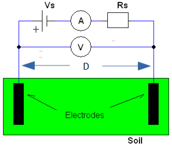
Figure 1.
The electrical soil resistivity setup for the 2-electrode method. is the internal resistance of the voltage source.
The above soil resistivity principle is also applied to a different and improved electrode arrangement, the Wenner structure. See Figure 2.

Figure 2.
The 4-point electrode configuration of the Wenner approach.
For the Wenner approach, where the geometric parameter k (1) is expressed in terms of the distance of the probes, the apparent soil resistivity is now given by [2]:
where a is the spacing of the probes (in meters). In this method, the lumped location of this apparent resistivity is at a depth of approximately . In field experimentation, the parameter a can be varied between a few centimeters and almost 30 m [2,4]. Indeed, there are other electrode distributions, such as the fall-of-potential, clamp-on, and Schlumberger methods. See [2] for more details. On the other hand, the non-contact method uses electromagnetic (EM) wave radiation propagation into the soil to study the reflected signals induced by the soil itself [16]. In contrast, capacitive resistivity is one of the techniques that extends the use of the resistivity method to an environment where the galvanic coupling of the electrodes is difficult (frozen ground, hard rocks, etc.). This technique allows rapid fieldwork without the galvanic coupling of electrodes. The main problem is the complicated calculation of the forward resistivity for a simple model [17]. The electrode–soil contact-based system has the advantages of not requiring user configuration and measuring at different soil depths [18]. Therefore, the non-contact EM system is lighter in weight, smaller in size, and, thus, easier to handle [19].
The paper’s main contributions can be split into two stages. First, a low-cost electronic system device able to detect variation in soil resistivity was designed. Second, a novel statistical data analysis method was introduced to study the soil resistivity. Our electronic circuit used a single-phase DC-to-AC converter followed by a transformer-to-soil-impedance coupling. This converter was operated at Hz. This value was set due to the transformer being rated at 50 Hz and due to the availability of electronic components for circuit realization. On the other hand, the proposed soil data method was based on the maximum likelihood statistical theory. This was employed to extract important soil data features to discriminate different soils’ resistivities. Additionally, a two-point soil experimental laboratory platform was also developed to support our findings. According to the experimental outcomes, our approach was effective at detecting dissimilar soil resistivities
The rest of the paper is structured as follows. Section 2 describes our electronic circuit for soil resistivity testing, whereas the proposed data processing approach is given in Section 3. Section 4 shows our experimental laboratory platform along with the obtained results to validate our principal contribution. Finally, Section 5 gives some conclusions.
2. Electronic Instrumentation
Our electronic instrumentation design was based on a DC-to-AC converter commonly employed in the field of power electronics [20], where we integrated a transformer to couple the soil resistivity to the device via the electrodes (see Figure 3). In this electronic circuit, the supplied complementary switching signals at the pins a and b came from an oscillating circuit, as shown in Figure 4. In other soil resistivity devices, the data measurement is performed at the probe level [2]. In our approach, we collected the data in the circuit excitation stage using the voltmeters and , respectively. Therefore, any change in the soil resistivity would be reflected in the primary stage of the transformer in the circuit. To complete the circuit description, in Figure 3, the transformer was connected following the format 15:230 V, the primary being 15 V and the secondary 230 V. Moreover, the oscillating circuit in Figure 4 used the basic free-running multi-vibrator scheme [21], and it was implemented using the operational amplifier Op1 (see Figure 4). We set k and μF. The resulting frequency oscillation was about Hz [21]. The rest of the circuit produced complementary commuting signals. Note that the voltmeter may also be used to evidence that the system is working properly.
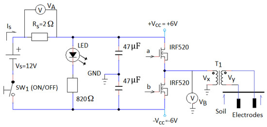
Figure 3.
The single-phase DC-to-AC converter followed by a transformer. This circuit receives complementary switching signals at the pins a and b, which are generated by the circuit shown in Figure 4.

Figure 4.
The circuit to produce the complementary switching signals at points a and b and then supplied to the DC-to-AC converter, as shown in Figure 3. The values R and C are programmed to tune the frequency of these commuting signals. The operational amplifiers Op1 and Op2 are realized by using the LM741C integrated circuit.
3. Design of the Experimental Soil Resistivity Platform
The measurement of soil resistivity samples can be performed in a laboratory [22,23,24,25,26,27]. To design our experimental soil resistivity platform by using the configuration of the two-point probes, we integrated a soil sample with the circuit, as shown in Figure 5. In this figure, in the aluminum container, we had some soil (the specimen or sample) with a different resistivity from the reference soil surrounding it. Hence, our soil resistivity meter should be able to distinguish among different soil specimens in this container. Figure 6 and Figure 7 present the overall experiment realization, including the electronic instrumentation part.
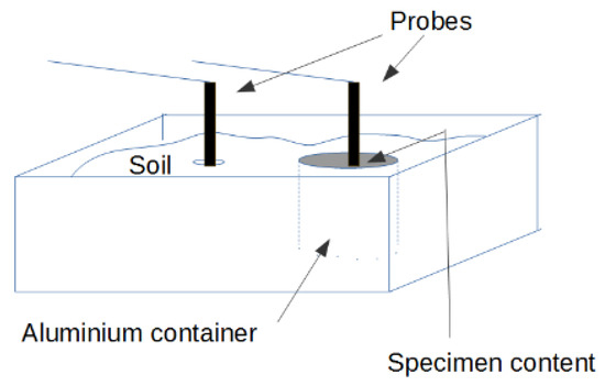
Figure 5.
Schematic description of our experimental soil platform. Important realization note: the electrode must not be in contact with the aluminum container.
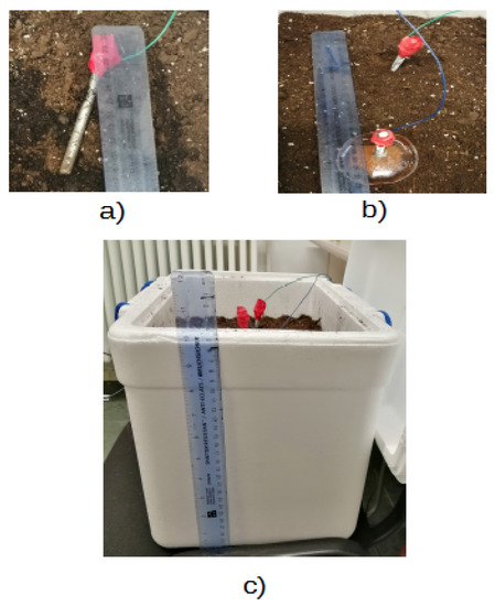
Figure 6.
Experimental soil platform: (a) a photo of an electrode; (b) a photo of both electrodes and the aluminum container; and (c) a front view of the realization.

Figure 7.
An overview of the soil resistivity experimental platform. The PicoScope device is a data-acquisition card, here employed to read the voltage values and via a computer.
4. The Soil Resistivity Data Analysis Approach
The proposed electronic device generated soil resistivity information given by the cited voltmeters and . These signals had some uncertainties due to several factors of the soil’s properties. Therefore, for the soil resistivity data analysis, we could assume that these signals had a uniform probability distribution, which can be represented by:
The main motivation for using the above expression was because, from the experimental point of view, the data were time varying, but bounded around a mean value. Therefore, the parameters and can be considered as indicators to distinguish different soil resistivities. For the distribution function (3), the method of moments was not useful to determine the parameters and . It can produce an estimated value of the parameter less than the maximum observed value and an estimation of the parameter greater than the observed minimum value [28]. Thus, the estimation of these parameters was carried out by using the maximum likelihood estimation method (MLE). The likelihood function for a sample of size n is [28]:
To estimate the parameters and from the sample data, we needed the maximum of the function (4). We may obtain this by solving the gradient vector equation: . Since the partial derivatives of the function (4) with respect to the parameters and were:
we had to determine when both equations were zero. However, since , the gradient never vanishes, so we could not use this method. Moreover, in Equation (5), the partial derivatives are both zero if and only if their denominators tend to infinity, that is when one of these two parameters tends to infinity with respect to the other. Therefore, to estimate these parameter values, we followed the MLE reasoning presented in [29]. From Equation (4), it is easy to see that the likelihood function tends to its maximum value when the difference is as small as possible. Given a sample of n observations and supposing that is the smallest and the largest one in the sample, in this case, cannot be greater than , and is less than . Therefore, the lowest positive value of is , and the maximum likelihood estimators for an n-sized sample are:
These estimations were important because the intermediate observations of a given sample were not considered, resulting in an effective analysis tool for soil resistivity diagnosis.
5. Experimental Results
In this section, we present three experimental settings for three different soil samples to study them from the resistivity point of view:
- Case 1: The aim of this first experiment was to detect a change from high to low resistivity by adding salty water to the aluminum container;
- Case 2: This experiment had the objective of measuring the change from high to medium resistivity by filling the aluminum container with sawdust;
- Case 3: The main objective of this scenario was to detect a resistivity change when the aluminum container was filled with cat litter.
In all cases, the experimental data were raw data, that is they were not obtained by any filtering process, so they had a certain randomness.
5.1. Case 1: Experiment with Salty Water
The experimental results related to measuring the change of the soil resistivity when the aluminum container was filled with salty water are shown in Figure 8. This case corresponded to a change in the soil specimen from high resistivity, the empty aluminum container, to a low one. This was because salty water is a conductive liquid. The experiment began when the electronic instrument was in the off position and then powered on at about 4 s. Later, the aluminum container was filled with salty water for 8 s. Therefore, this process ended around 12 s, as shown in the Voltmeter A and B diagrams. See Figure 8. To test our data analysis method, we performed the statistical parameter estimation presented in (6) on the data collected from the experiment. This was done by setting , corresponding to approximately s of data acquisition from our experiment; a moving window of size n was applied, and then, Equation (6) was used for each window up to the end of the data file. The first 100 data were used, then the second set of 100 data, and so on. Figure 9 proves that our instrument and data analysis approach were sensitive to soil resistivity variation.
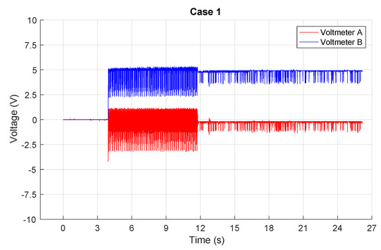
Figure 8.
Case 1: Experimental results. During approximately 8 s (from approximately 4 s to 12 s), we filled the container with salty water, then stopped. The voltmeter detected this change of salinity with a small delay.
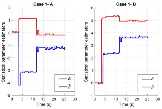
Figure 9.
Case 1: Data analysis evolution of the likelihood estimation of the decision parameters and (6). At approximately 12 s, both parameters detected different soil resistivities.
5.2. Case 2: Experiment with Sawdust
In this case, the previous experiment was repeated, but now, the container was filled with sawdust. Figure 10 presents the experimental outcomes related to measuring the soil resistivity variation when the aluminum container was being filled. This example corresponded to a change in the soil specimen from a high-resistivity scenario to a medium-resistivity event. This experimental testing again started with the instrument in the off position, then powered on at about s. Later, the aluminum container was filled with the sawdust. This process ended at around 14 s. Figure 11 shows the corresponding data processing result as in the previous experiment. From Figure 11, we proved that our instrument and data analysis approach were sensitive to soil resistivity variation. However, it should be noted that, in this case, the parameter was more sensitive than the other. In this case, the change of soil resistivity was hard to detect from the voltmeter diagrams (see Figure 10), but it can be appreciated from the data analysis, as shown in Figure 11. Finally, Figure 12 shows the aluminum container filled with the sawdust.

Figure 10.
Case 2: Experimental results, where a change in soil resistivity is hard to read.

Figure 11.
Case 2: Time evolution of the likelihood estimation of the parameters and . Case 2-A shows, at approximately 14 s, that parameter detected a change in soil resistivity.

Figure 12.
Case 2: The aluminum container filled with wood sawdust.
5.3. Case 3: Experiment with Cat Litter
In this last experiment, we repeated the same experimental process, but using cat litter. Now, the aim was to obtain a dynamic detection system for resistivity, and the cat litter met our goal due to its granular texture. The corresponding experimental outcomes are shown in Figure 13, Figure 14 and Figure 15. Once again, our instrument and data analysis approach were also sensitive to this soil resistivity variation.
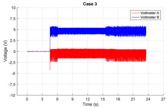
Figure 13.
Case 3: Experimental results. During approximately 9 s, the aluminum container was filled with cat litter, as the voltmeter diagrams evidence.
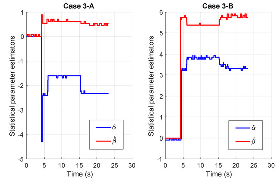
Figure 14.
Case 3: Time evolution of the likelihood estimation of the parameters and . As for the previous scenarios, the parameters confirmed the detection of soil resistivity changes.
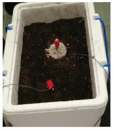
Figure 15.
Case 3: The aluminum container filled with cat litter.
6. Conclusions
In this paper, an electronic device for soil resistivity analysis was developed. Our design was conceived as a soil instrument to measure the variability of soil resistivity. This included a pilot experimental platform to validate our contribution, followed by a data processing method based on the MLE technique. According to our experimental outcomes, our approach was able to detect soil resistivity variations. Therefore, when both voltmeter readings were unable to discern a change in the soil resistivity, the proposed MLE approach was able to. Therefore, from the numerical point of view, a model of a random dataset was developed and used for data diagnosis. Hence, the and parameters can be used as features for dataset comparison. Finally, this approach was low in cost.
Author Contributions
Conceptualization, L.A., G.P.-V. and J.G.-B.; methodology, L.A.; software, L.A., G.P.-V. and J.G.-B.; validation, L.A.; formal analysis, J.G.-B.; investigation, L.A.; resources, G.P.-V.; data curation, J.G.-B.; writing—original draft preparation, L.A., G.P.-V. and J.G.-B.; writing—review and editing, J.G.-B.; supervision, L.A. All authors read and agreed to the published version of the manuscript.
Funding
This research was funded by the Ministry of Economy, Industry and Competitiveness, State Research Agency of the Spanish Government through Grant DPI2016-77407-P (MINECO/AEI/FEDER, UE).
Data Availability Statement
Data supporting the reported results can be supplied by the authors.
Conflicts of Interest
The authors declare no conflict of interest.
Abbreviations
The following abbreviations are used in this manuscript:
| AC | Alternating current |
| DC | Direct current |
| EM | Electromagnetic |
| MLE | Maximum likelihood estimation method |
References
- Wenner, F. A Method of Measuring Earth Resistivity. Bull. Bur. Stand. 1916, 12, 469–478. [Google Scholar] [CrossRef]
- Samouelian, A.; Cousin, I.; Tabbagh, A.; Bruand, A.; Guy, R. Electrical resistivity survey in soil science: A review. Soil Tillage Res. 2005, 83, 173–193. [Google Scholar] [CrossRef]
- Loke, M.H.; Chambers, J.E.; Kuras, O. Instrumentation, electrical resistivity. Encycl. Solid Earth Geophys. 2011, 1, 599–604. [Google Scholar]
- Igboama, W.N.; Ugwu, N.U. Fabrication of resistivity meter and its evaluation. Am. J. Sci. Ind. Res. 2011, 2, 713–717. [Google Scholar]
- Chen, T.T.; Hung, Y.C.; Hsueh, M.W.; Yeh, Y.H.; Weng, K.W. Evaluating the Application of Electrical Resistivity Tomography for Investigating Seawater Intrusion. Electronics 2018, 7, 107. [Google Scholar] [CrossRef]
- Bodh, R.; Shrivastava, P.; Shrivastava, S. Application of Schlumberger Method for Characterization of Soil. Int. J. Innov. Technol. Explor. Eng. 2019, 8. [Google Scholar] [CrossRef]
- Han, Y.; Yang, W.; Li, M.; Meng, C. Comparative Study of Two Soil Conductivity Meters Based on the Principle of Current-Voltage Four-Terminal Method. IFAC-PapersOnLine 2019, 52, 36–42. [Google Scholar] [CrossRef]
- Kaminskyj, R.; Shakhovska, N.; Michal, G.; Ladanivskyy, B.; Savkiv, L. An Express Algorithm for Transient Electromagnetic Data Interpretation. Electronics 2020, 9, 354. [Google Scholar] [CrossRef]
- Ramos-Leanos, O.; Uribe, F.; Valcárcel, L.; Hajiaboli, A.; Franiatte, S.; Dawalibi, F. Nonlinear Electrode Arrangements for Multilayer Soil Resistivity Measurements. IEEE Trans. Electromagn. Compat. 2020, 62, 2148–2155. [Google Scholar] [CrossRef]
- Huda, E.; Yohandri, E. Development of an automatic multi-electrode digital resistivity meter for the Schlumberger configuration. Pillar Phys. 2020, 13, 74–81. [Google Scholar]
- Petrache, E.; Dick, E.; Jamali, B.; Chisholm, W. Soil Resistivity Testing; CEATI Report T113700-3702; CEATI International: Montreal, QC, Canada, 2014. [Google Scholar]
- Southey, R.; Siahrang, M.; Fortin, S.; Dawalibi, F. Using Fall-of-Potential Measurements to Improve Deep Soil Resistivity Estimates. IEEE Trans. Ind. Appl. 2015, 51, 5023–5029. [Google Scholar] [CrossRef]
- Permal, N.; Osman, M.; Kadir, M.Z.A.A.; Ariffin, A. Review of Substation Grounding System Behavior Under High Frequency and Transient Faults in Uniform Soil. IEEE Access 2020, 8, 142468–142482. [Google Scholar] [CrossRef]
- Supandi, S. Geotechnical profiling of a surface mine waste dump using 2D Wenner–Schlumberger configuration. Open Geosci. 2021, 13, 335–344. [Google Scholar] [CrossRef]
- Sophocleous, M. Electrical Resistivity Sensing Methods and Implications. Electr. Resist. Conduct. 2017, 5, 67748. [Google Scholar]
- Unal, I.; Kabas, O.; Sozer, S. Real-Time Electrical Resistivity Measurement and Mapping Platform of the Soils with an Autonomous Robot for Precision Farming Applications. Sensors 2020, 20, 251. [Google Scholar] [CrossRef] [PubMed]
- Gruzdev, A.; Bobachev, A.; Shevnin, V. Determining the Field of Application of the Noncontact Resistivity Technique. Mosc. Univ. Geol. Bull. 2020, 75, 644–651. [Google Scholar] [CrossRef]
- Sudduth, K.; Kitchen, N.; Bollero, G.; Bullock, D.; Wiebold, W. Comparison of electromagnetic induction and direct sensing of soil electrical conductivity. Agron. J. 2003, 95, 472–482. [Google Scholar] [CrossRef]
- Lueck, E.; Ruehlmann, J. Resistivity Mapping with GEOPHILUS ELECTRICUS—Information about Lateral and Vertical Soil Heterogeneity. Geoderma 2013, 199, 2–11. [Google Scholar] [CrossRef]
- Rashid, M. Power Electronics: Circuits, Devices, and Applications, 3rd ed.; Pearson: London, UK, 2003. [Google Scholar]
- Franco, S. Design with Operational Amplifiers and Analog Integrated Circuits, 2nd ed.; McGraw-Hill: New York, NY, USA, 2002. [Google Scholar]
- Archie, G. The electric resistivity log as an aid in determining some reservoir characteristics. Trans. Am. Inst. Min. Metall. Pet. Eng. 1942, 146, 54–62. [Google Scholar]
- Zhou, M.; Wang, J.; Cai, L.; Fan, Y.; Zheng, Z. Laboratory Investigations on Factors Affecting Soil Electrical Resistivity and the Measurement. IEEE Trans. Ind. Appl. 2015, 51, 5358–5365. [Google Scholar] [CrossRef]
- Datsios, Z.; Mikropoulos, P.; Karakousis, I. Laboratory characterization and modeling of DC electrical resistivity of sandy soil with variable water resistivity and content. IEEE Trans. Dielectr. Electr. Insul. 2017, 24, 3063–3072. [Google Scholar] [CrossRef]
- Roodposhti, H.; Hafizi, M.; Kermani, M.; Nik, M. Electrical resistivity method for water content and compaction evaluation, a laboratory test on construction material. J. Appl. Geophys. 2019, 168, 49–58. [Google Scholar] [CrossRef]
- Kouchaki, B.; Bernhardt-Barry, M.; Wood, C.; Moody, T.A. Laboratory Investigation of Factors Influencing the Electrical Resistivity of Different Soil Types. Geotech. Test. J. 2019, 42, 829–853. [Google Scholar] [CrossRef]
- Adla, S.; Rai, N.; Sri Karumanchi, H.; Tripathi, S.; Disse, M.; Pande, S. Laboratory Calibration and Performance Evaluation of Low-Cost Capacitive and Very Low-Cost Resistive Soil Moisture Sensors. Sensors 2020, 20, 363. [Google Scholar] [CrossRef]
- Benjamin, J.; Cornell, C. Probability, Statistics, and Decision for Civil Engineers; McGraw-Hill: New York, NY, USA, 2014. [Google Scholar]
- Mood, A.; Graybill, F. Introduction to the Theory of Statistics; McGraw-Hill: New York, NY, USA, 1963. [Google Scholar]


Publisher’s Note: MDPI stays neutral with regard to jurisdictional claims in published maps and institutional affiliations. |
© 2021 by the authors. Licensee MDPI, Basel, Switzerland. This article is an open access article distributed under the terms and conditions of the Creative Commons Attribution (CC BY) license (https://creativecommons.org/licenses/by/4.0/).