Abstract
In this paper we introduce an approach to accelerate many-scenario (i.e., hundreds to thousands) power system simulations which is based on a highly scalable and flexible open-source software environment. In this approach, the parallel execution of simulations follows the single program, multiple data (SPMD) paradigm, where the dynamic simulation program is executed in parallel and takes different inputs to generate different scenarios. The power system is modeled using an existing Modelica library and compiled to a simulation executable using the OpenModelica Compiler. Furthermore, the parallel simulation is performed with the aid of a message-passing interface (MPI) and the approach includes dynamic workload balancing. Finally, benchmarks with the simulation environment are performed on high-performance computing (HPC) clusters with four test cases. The results show high scalability and a considerable parallel speedup of the proposed approach in the simulation of all scenarios.
1. Introduction
Power systems are experiencing rapid transitions lead by the increasing level of renewable power generation and by their progressive digitalization. The classical power system architecture centered around large generation units with very controllable power production is progressively evolving towards a model with more distributed generation based on renewable sources that are inherently less controllable. Moreover, renewable sources such as wind and solar are interfaced to the grid via power converters. Thus, the decommissioning of thermal power plants with synchronous machines and their replacement with converter interfaced generation leads to a gradual reduction of system inertia. Both the lower level of rotating inertia in the power systems and the higher variability of the power generation are expected to render future power systems more difficult to operate because the margins to counteract contingency events will be tighter. These trends challenge the role of transmission system operators that would need to introduce innovative technologies in their control rooms to ensure sufficient levels of power system security.
1.1. Motivation
The present digitalization trend is affecting power systems, especially in terms of wide area monitoring. A growing number of phasor measurement units (PMUs) are deployed in the power systems offering the possibility to collect synchronized measurements over a geographically extended area with a refresh rate that is one or two orders of magnitudes higher than with traditional supervisory control and data acquisition (SCADA) solutions. This is accompanied by a stronger communication infrastructure and more affordable computation capabilities that have the potential to improve the control capabilities.
The transmission system operators (TSOs) continuously monitor the power systems and should rapidly react to contingencies in order to mitigate their consequences. These mitigation actions are classically implemented as protective functions based on precalculated scenarios or as manual actions based on the experience of the operators. A better decision support could be provided by processing the available information with real-time simulation of the power systems. However, the number of cases to be evaluated to offer a comprehensive evaluation can be easily very large and exceeding what can be computed sequentially in a practically reasonable time-frame: A total number of system configurations required for an n-2 contingency analysis in [1] is 81,003, considering the different operation status of the power system per 15 in a day, scenarios are generated. Suppose each simulation takes 10 s, simulating all these scenarios sequentially would need 2.5 years. In addition to the needs of the TSOs, studies in distribution grid need dynamic simulation of a large number of scenarios as well [2,3]. This justifies the value of being able to perform and simulate a large set of scenarios in parallel. Moreover, to accelerate power system research, there is a need for open and fast tools. As an example, artificial intelligence (AI)-related power system studies have received increased attention lately. For the AI methods to be applicable, however, large data sets of high quality are needed [4].
1.2. Related Works
With the rising need of computing power, high-performance computing (HPC) techniques have been exploited for many years to accelerate power system studies. The survey [5] reviewed a variety of HPC applications in power system studies like contingency analysis, reliability analysis, transient stability simulation, state estimation, power flow simulation, etc. Other techniques such as e.g., cloud computing have gain grounds in wide area monitoring [6] to facilitate data acquisition, sharing, and processing.
In the power system community, tools that allow parallel dynamic simulation of multiple scenarios have existed for a while. Among these, available commercial tools [7,8] are made for TSOs for dynamic security assessment (DSA) that provides parallel simulation of different scenarios but they can be less flexible for other purposes. For instance, the parallel simulation part cannot be reprogrammed or extended by users freely. Tools as presented in [9,10] provide parallel simulation of multiple scenarios through several instantiations of simulation software on the same machine. These approaches are limited mainly because the simulations can only be performed on a single computer and, in case of commercial simulation software, the availability of licenses, e.g., licenses are needed for each simulation process [10]. In [11], the tool in [10] is updated to support execution on HPC clusters. However, since the simulation backend is in fact a commercial simulator, some limitations still remain.
In [12], the authors developed an approach that is capable of performing parallel dynamic simulations on computer clusters, offering dynamic workload balancing as well. However, this approach might not be general enough for the power system community to facilitate a large-scale parallel simulation of different scenarios. This is because the approach is implemented on a customized power system simulator that has not been published.
1.3. Contribution of This Work
The many-scenario approach introduced in this paper is based on the single program, multiple data (SPMD) paradigm to parallelize power system dynamic simulations. Instead of multiple instantiations of the whole simulation suite, only the computing task, i.e., the compiled simulation executable, is instantiated multiple times. In this way, a compilation of the simulation executables for different scenarios is avoided. With the aid of message-passing interface (MPI), simulation tasks can be distributed on a HPC computer cluster, enabling the parallel simulation of hundreds to thousands of scenarios. Furthermore, to balance computational workload among simulation processes, a dynamic workload balancing strategy is provided based on the classic manager-worker paradigm [13].
Another highlight of the proposed approach lies in the modeling of the power system which takes advantage of the object-oriented equation-based programming language Modelica. Models can be implemented using existing Modelica libraries, yielding a high degree of freedom in terms of modeling. As a result, not only are the models implemented with different libraries reused, but also the simulation capabilities are extended through different Modelica libraries, e.g., dynamic simulations with the electro-magnetic transient (EMT), static phasor (SP), and even the dynamic phasor (DP) domain.
To further increase the flexibility in modeling, the open-source project CIMverter [14] has been integrated which allows conversion from the widely-used Common Information Model (CIM) respectively, Common Grid Model Exchange Standard (CGMES) documents to Modelica system models based on different Modelica libraries. We have provided a flexible way based on a well-known programming language instead of a domain specific language (DSL) to define different scenarios, for which we chose Python.
Based on these approaches and tools, the parallel power system simulation module htcsim (high-throughput computing SIMulation) was implemented. In addition, although the proposed approach was realized through multiple open-source projects, it can be applied also for commercial simulation software that is not open source. The requirements are that the used computer system has an MPI implementation which is the case for all modern HPC clusters and supercomputers. Moreover, the simulation software needs to support batch execution, e.g., from a command line. Moreover, it needs to provide a functionality (e.g., through input files or an API like OMPython) to run a simulation for different parameters depending on the scenario to be simulated. Examples for such commercial software are Dymola, PSS/E, and PowerFactory. In the end, as always in the case of commercial software, a proper license that allows the parallel simulation on many nodes is needed for these tools.
2. The Many-Scenario Approach for Parallel Dynamic Simulations
2.1. Fundamentals
Before introducing the concept of our approach and its implementation, details of the utilized tools, OpenModelica, and MPI, as well as fundamentals of power system simulation are reviewed in the following subsections.
2.1.1. Modelica
Modelica is an equation-based language which enables modeling in a declarative way through mathematical equations instead of an imperative way with variable assignments. Equations allow engineers to focus on the formulation of the physical model [15]. Therefore, the flexibility and reusability of the Modelica models is increased. The existing Modelica environments, such as OpenModelica, also provide various solvers that relieve engineers from numerical implementations.
There already exist several Modelica libraries that support the modeling and simulation of power systems, such as ModPowerSystems [16], PowerGrids [17], and PowerSystems [18] etc. These libraries provide electrical component models as Modelica classes, where necessary equations are encapsulated. In order to build a power grid, instances of different components can be connected to a system model, such that their equations are combined.
When a Modelica model is built, the process of translation consists of several steps as sketched in Figure 1: First, the source code is translated into an internal representation, e.g., an abstract syntax tree (AST). This representation is then analyzed and converted into a set of equations, constants, variables, and function definitions. This process is called flattening in Modelica.
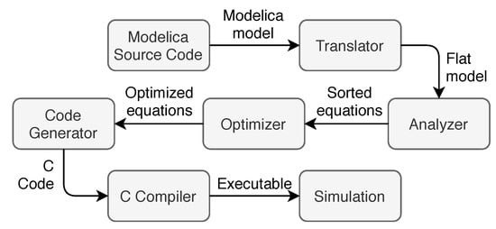
Figure 1.
Simulation generation by OpenModelica.
The resulting equations of the flattening process are then sorted and optimized to obtain a minimum set of equations that will eventually be solved by the numerical solver. Afterwards, the explicit equation set is converted into C code and finally compiled to an executable. In the meantime, a configuration file based on the extensible markup language (XML) is generated, containing simulation configurations and initial value of the simulation variables. The generated executable is linked to numerical libraries (provided by the Modelica environment such as OpenModelica). During its runtime, the program reads in the configuration file to determine the chosen numerical solver, simulation time step, etc. as well as the initial values for the variables to perform the simulation.
2.1.2. Message-Passing Interface (MPI)
MPI is a portable standard designed to function on a wide variety of parallel computers, especially for distributed-memory architectures. The implementation of MPI follows the message-passing model [13], where the same program is executed by different processes simultaneously (according to the SPMD paradim). However, since each of the process has a unique ID number, referred to as rank, different processes may perform different operations (depending on the rank) during the program’s runtime. Each process performs local computations with its own variables and exchange data with I/O devices or other processes using MPI calls.
For this purpose, MPI defines the syntax and semantics for library routines and allows users to write parallel programs with the message-passing model in the chosen programming languages (i.e., often C, C++, or Fortran). In this work, the Python package mpi4py is used as the MPI implementation. It provides an object-oriented approach to message passing which grounds on the standard MPI-2 C++ bindings. The interface was designed with focus on translating MPI syntax and semantics of standard MPI-2 bindings for C++ to Python [19].
2.1.3. Power System Simulation
We would like to give here a brief review of the static and dynamic simulation of power system. For static simulation of the power system, one typically uses a power flow simulation, where the system is assumed to be at a certain steady state. Therefore, a set of non-linear algebraic equations is solved. The result of power flow simulation yields the value of all system states, i.e., nodal voltage amplitudes and phase angles, based on the given generation, consumption, and of course the topology of the system. A dynamic simulation of power systems solves differential-algebraic systems of equations (DAEs) where the equations are solved at every chosen point in time. In general, dynamic simulations can be initialized with the results of a power flow simulation, so that the system is initialized at a given steady state that fulfills algebraic constraints.
2.2. Concept
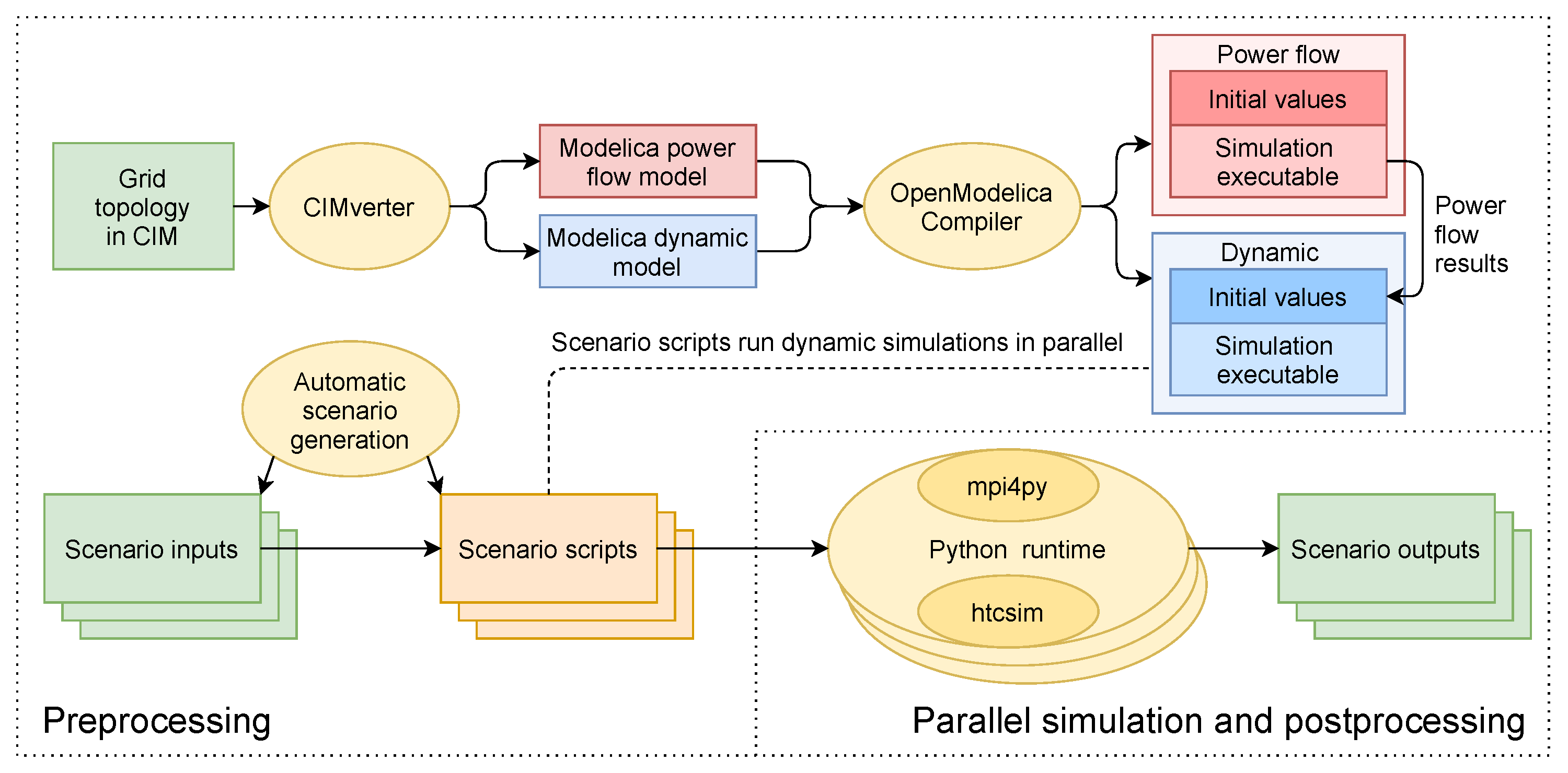
The concept of the proposed many-scenario approach is depicted in Figure 2, in which the overall workflow can be categorized into three procedures: Preprocessing, parallel simulation, and postprocessing.

Figure 2.
Overall concept of the htcsim-based environment for parallel scenario simulation.
2.2.1. Preprocessing
The preprocessing is illustrated in the upper and bottom left part, which contains the creation of the Modelica models of the power system, the compilation of associated simulation executables, and the generation of scenario inputs and scripts. This procedure is performed only once before the simulations. As a result, all necessary files for the parallel simulation are prepared.
In Figure 2, the workflow starts by assuming that CIM documents of a power system model are provided. At the beginning, two Modelica models are created by the CIMverter tool using the CIM documents; namely the Modelica power flow model and the Modelica dynamic model. The latter is used for dynamic simulation and will be executed by multiple so-called worker processes to perform parallel simulation analogously to the SPMD paradigm. Certainly, the conversion step of CIM documents to Modelica models can be skipped if the two Modelica models already exist.
The Modelica power flow model is used to initialize the dynamic simulation as explained in Section 2.1.3. It conducts an AC type power flow. These two Modelica models are then compiled by OpenModelica Compiler (OMC) to generate simulation executables with their associated configuration files as introduced in Section 2.1.1, which contain initial values of all variables. After that, the compiled Modelica power flow model is executed, whose results are then read by htcsim to replace the chosen variables, e.g., nodal voltage amplitudes and phase angles, in the generated configuration file by compiling the Modelica dynamic model. As a result, when the simulation executable generated by compiling the Modelica dynamic model is executed, it will read the configuration file with updated initial values. In this way, the dynamic simulation has been initialized to a certain steady state.
In addition, the initialization of a dynamic simulation with power flow results would not affect the overall simulation time since it takes place prior to the parallel simulation. Moreover, the power flow simulation does not have to be repeatedly performed for each scenario’s steady-state initialization even if the operating points are changed. As in Modelica libraries, like PowerGrids, the implemented initial equations [17] in dynamic components, with the use of the homotopy method [20], ensures a steady-state initialization for dynamic simulation. The pre-calculated power flow results can be taken by the initial equations as a starting point to calculate the steady-state. Therefore, it has a limited contribution to the preprocessing time too.
The bottom left part shows the generation of scenario inputs and scripts. Scenario inputs are the various inputs to the simulation executable analogously to the data in the SPMD paradigm. The simulation executable is able to read these inputs as instructions to make certain the power system component performs different behaviors. For example, a time series of ones and zeros can be read by a circuit breaker component to determine whether it is closed or open at any point in time.
By providing different scenario inputs, various events can be created. In general, states and topologies of power systems are affected or directly described by simulation variables such as controller parameters, breaker states, system frequencies, etc. This allows the creation of a wide variety of events by manipulating simulation variables, for instance, common events such as switching, load changes, etc. Furthermore, by utilizing Modelica’s algorithm sections, complex control algorithms can be realized within the models (i.e., eventually in the simulation executables) in an imperative way.
At this stage, parallel simulation can already be performed based on the dynamic simulation executable and scenario inputs. Scenario scripts are introduced to provide higher flexibility. To this end, a script, referred to as scenario script, is generated for each scenario which contains a necessary code to run the simulation executable with specific inputs. Therefore, each scenario can be simulated individually if needed without initiating the whole parallel simulation framework. Furthermore, with a specific script per scenario, complex operations can be performed on the simulation results during parallel simulation or after, where the latter is introduced in our concept as postprocessing.
Finally, as common with MPI, all the generated files are placed on a distributed file system that can be accessed by any node (i.e., computer) in the computer cluster.
2.2.2. Parallel Simulation
The parallel simulation can be performed based on the files and code generated from preprocessing. It follows an SPMD paradigm, where the dynamic simulation executable is executed by multiple processes in parallel with the aid of MPI, and different scenarios are created by reading different scenario inputs. It can be noticed that since the parallelized part equals the simulation of separate scenarios, the obtained simulation results are the same as if these scenarios were simulated sequentially.
2.2.3. Postprocessing
The postprocessing is intended to give preliminary data processing with the simulation results. This is performed through scenario scripts. Therefore, computationally intensive simulation result processing can be carried out subsequently to a simulation in parallel as well. A postprocessing can be added to the scenario scripts as well which decides if additional scenarios need to be simulated. If so, further scenario scripts can be generated and executed after the execution of all original scenarios.
2.3. Implementation
To implement the proposed approach, the parallel simulation module htcsim has been developed. The motivation of choosing Python as the programming language comes from the fact that the most time-critical part is the dynamic simulation itself, which is already translated to efficient C code, while the rest of the tasks are related to scenario generation, compilation, task distribution to the parallel processes, input/output, user interaction, etc. These tasks are non-time critical as they are performed prior to simulation or require comparatively very little time. Therefore, they can be managed by a Python program.
The interpreted high-level language Python provides high flexibility, is well-established, and requires lower learning efforts. Therefore, it is advantageous for the abovementioned management tasks, i.e., defined in the scenario scripts.
2.3.1. Scenario Script and Input
As introduced in Section 2.2, scenario inputs are the input data to the simulation executable for simulating different scenarios, whereas the scenario scripts handle the executions. Regardless of the postprocessing, scenario scripts shares high similarity. Therefore, techniques such as templating can be applied to generate those scripts.
The current implementation of a scenario script contains three parts. In the first part, several assignment statements are defined: The scenario name, model name, and paths of the simulation configuration file, etc. In the second part, the configuration file is copied into the scenario directory and parsed by an XML parser. The absolute path to each scenario input is added to the components in the Modelica model that requires an external input. Alternatively, this procedure can be freed by designing a certain naming convention for the input files and use their relative paths in the Modelica components. Subsequently, the simulation executable is executed by the script with the modified configuration. The last part reads the simulation results and performs certain processing that can be modified by the user, e.g., plotting a diagram regarding the evolution of selected variables over time and saving it to the appropriate scenario directory.
Scenario inputs can be, e.g., text files storing time tables using a format readable by the Modelica.Blocks.Sources.CombiTimeTable component, which converts the input time table into time series that can be used by other Modelica components. To automatize the generation of this data, a Python script is implemented that generates time tables following specific patterns according to the type and occurrence of the event specified by the user. The selection of events can be automatized by more generic methods such as event trees [21] that could consider uncertainty as well.
2.3.2. Executable Generation
The generation of simulation executables is realized with the OMC. In practice, this procedure is automatized via a Python package OMPython, which is the Python interface of OpenModelica. With this package, an interaction between the Python script and OMC can be established. Moreover, commands following the OpenModelica scripting syntax are generated in the script and sent to the OMC to build the executable.
2.3.3. Computational Workload Balancing
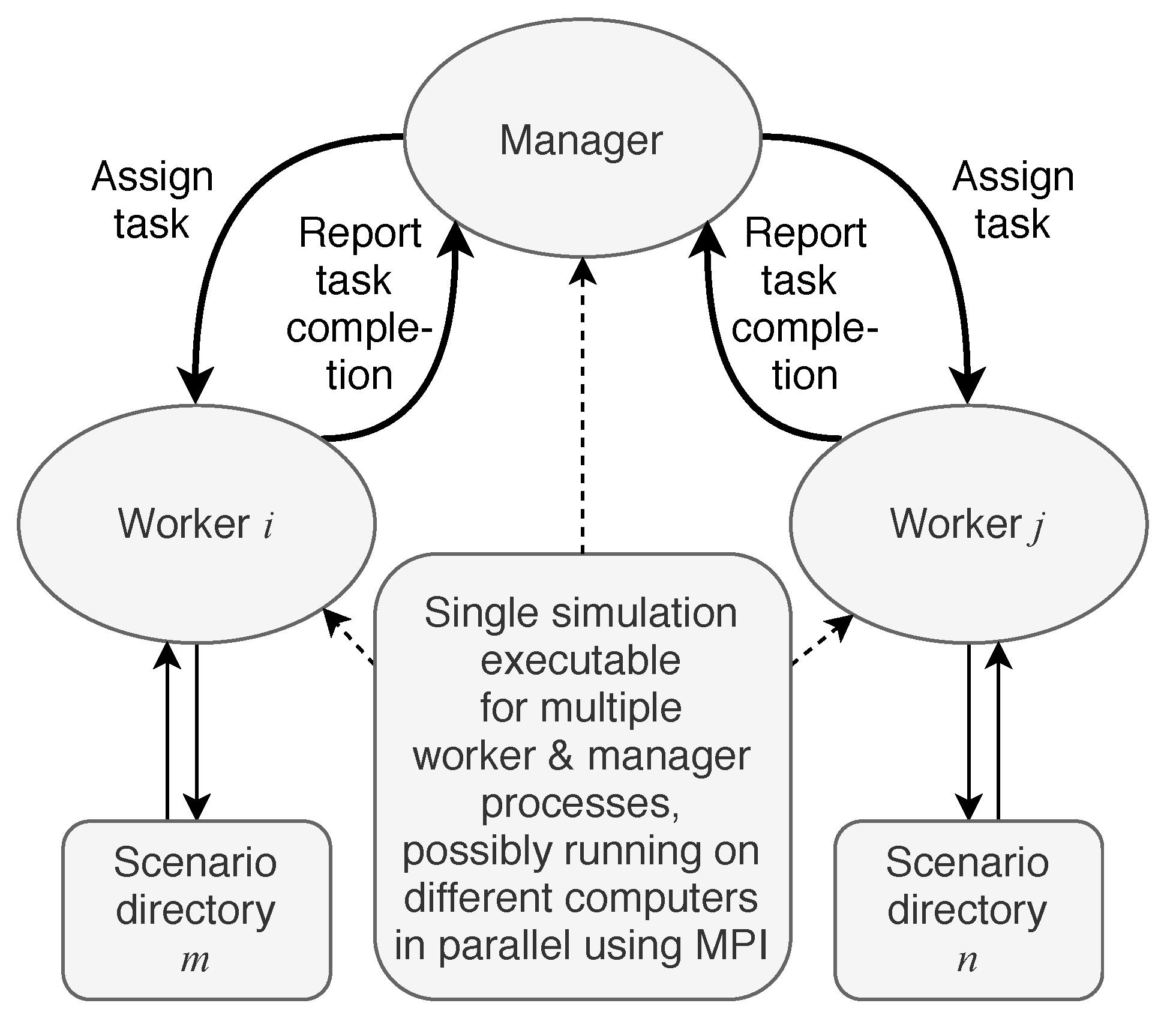
To balance the computational workload among simulation processes, a dynamic balancing strategy based on the manager-worker paradigm is applied. It is implemented using the Python MPI package mpi4py to support run-time allocation of tasks to processes. In the htcsim implementation, the task is the index of the scenario that needs to be simulated. During the parallel simulation, the so-called manager process is responsible for keeping track of tasks. It assigns tasks to the available worker processes which execute tasks (i.e., the dynamic simulation executable on the appropriate scenario inputs) and return feedback regarding the tasks’ completion to the manager. This interaction between the manager and the workers is depicted in Figure 3. When a worker receives a task message from the manager, in our case the scenario index, it changes its working directory to the corresponding scenario directory and executes the scenario script. After completion, it sends a message to the manager, which can assign a new task to the worker and so forth.

Figure 3.
Manager-worker paradigm.
This strategy ensures a certain workload balance among processes which minimizes the idle time of each processor without an a priori knowledge of the scenario execution times. A worker process exits when it completes a task and the manager has no more tasks to assign. At this point, no worker has more than one task left to complete. Although only a single manager process exists, it is merely passing scenario indices to the worker processes to start relatively long simulations. Therefore, it is in practice not a bottleneck for the execution time of the parallel simulation. Furthermore, this balancing strategy requires no communication among worker processes which reduces communication overhead thus beneficial to the parallel speedup.
3. Experiment and Discussion
The benchmarks were performed on two HPC clusters. For test cases 1 to 3, the CLAIX-2018 cluster of RWTH Aachen University (Aachen, Germany) with around 1250 computer nodes was used, where each node has two Intel Xeon Platinum 8160 Processors (2.1 GHz) installed, providing 48 physical cores per node. Hyper-Threading is disabled by default on every node. Each node has at least 4 GB of main memory per core. The nodes have a CentOS 7 server Linux installed with kernel 3.10.0-1127.19.1.el7.x86_64.
Test case 4 was executed on the standard compute nodes of the JURECA supercomputer at Forschungszentrum Jülich (Jülich, Germany), where 480 nodes with two AMD EPYC 7742 CPUs (2.25 GHz) are installed, providing 128 cores per node. The nodes have a CentOS 8 server Linux installed with kernel 4.18.0-240.22.1.el8_3.x86_64.
Four test cases are presented in the following. In test case 1 and 3, scalability benchmarks of our approach were performed based on different load step scenarios on two networks with different complexity, i.e., the two-area system [22] and the IEEE 14-bus system [23]. In test case 2, a dynamic contingency simulation considering different operating states was performed with our approach based on the two-area system in test case 1, the parallel speedup provided by our approach was calculated. In test case 4, the scalability benchmark is performed on a larger system with 10,000 different scenarios, where islanded grids are interconnecting with each other during the simulation. The parallel speedup is calculated as in test case 2.
At this point we would also like to point out that in our approach it is not a matter of parallelizing the calculations of a single scenario or model. This is already the subject of other research activities [24]. Therefore, the size of the models does not play a role for the parallel speedup of our approach.
3.1. Test Case 1
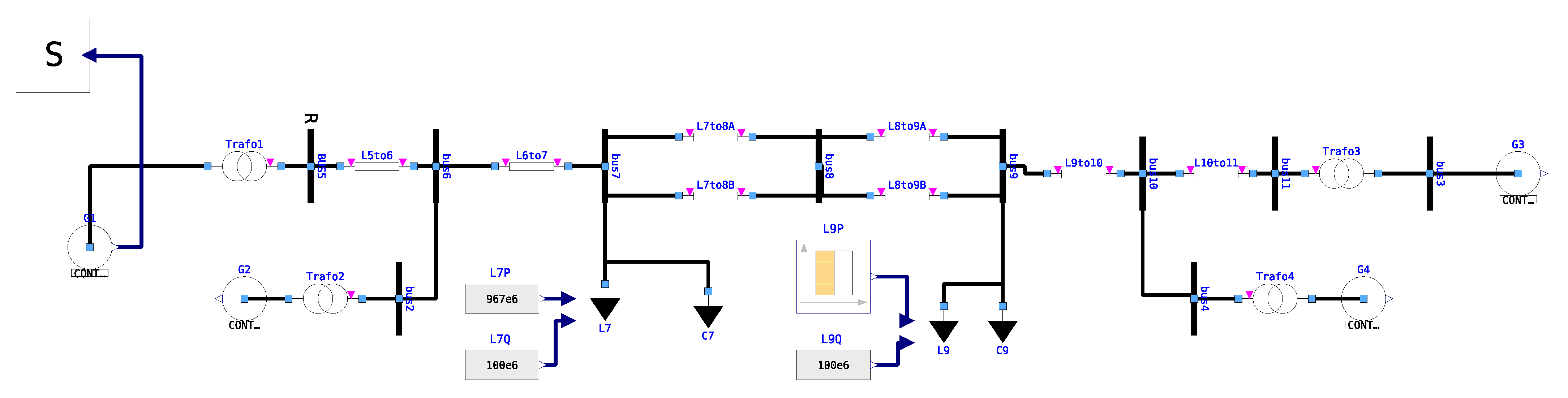
The two-area system model [22] shown in Figure 4 is built in OpenModelica with the PowerGrids library. In this model, all the synchronous machines are implemented equivalently to the model described in [22] provided by the PowerGrids library, and are equipped with the turbine governor IEEE TGOV1, the automatic voltage regulator IEEE AV4A, and the power system stabilizer IEEE PSS2A. A large disturbance caused by a load step is performed on load L9. The load step event is set with a magnitude of 56.6% of the original load and each event consists of an up step and a down step. The load step event is replicated 10 times during each simulation with the same interval between every events. To represent a realistic simulation duration, the simulation duration is configured to 10 .
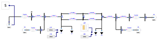
Figure 4.
Two-area-system model from [22] implemented using PowerGrids in OpenModelica.
The simulation is performed with the SUNDIALS IDA solver [25] with a simulation time step of 1 . Scenarios are distinguished by having a different starting time of a series of 10 load step events. In the end, up to 256 scenarios are generated and simulated. In addition, the parallel simulation is configured to always use the same number of worker processes as the number of scenarios and each MPI process is allocated to different nodes.
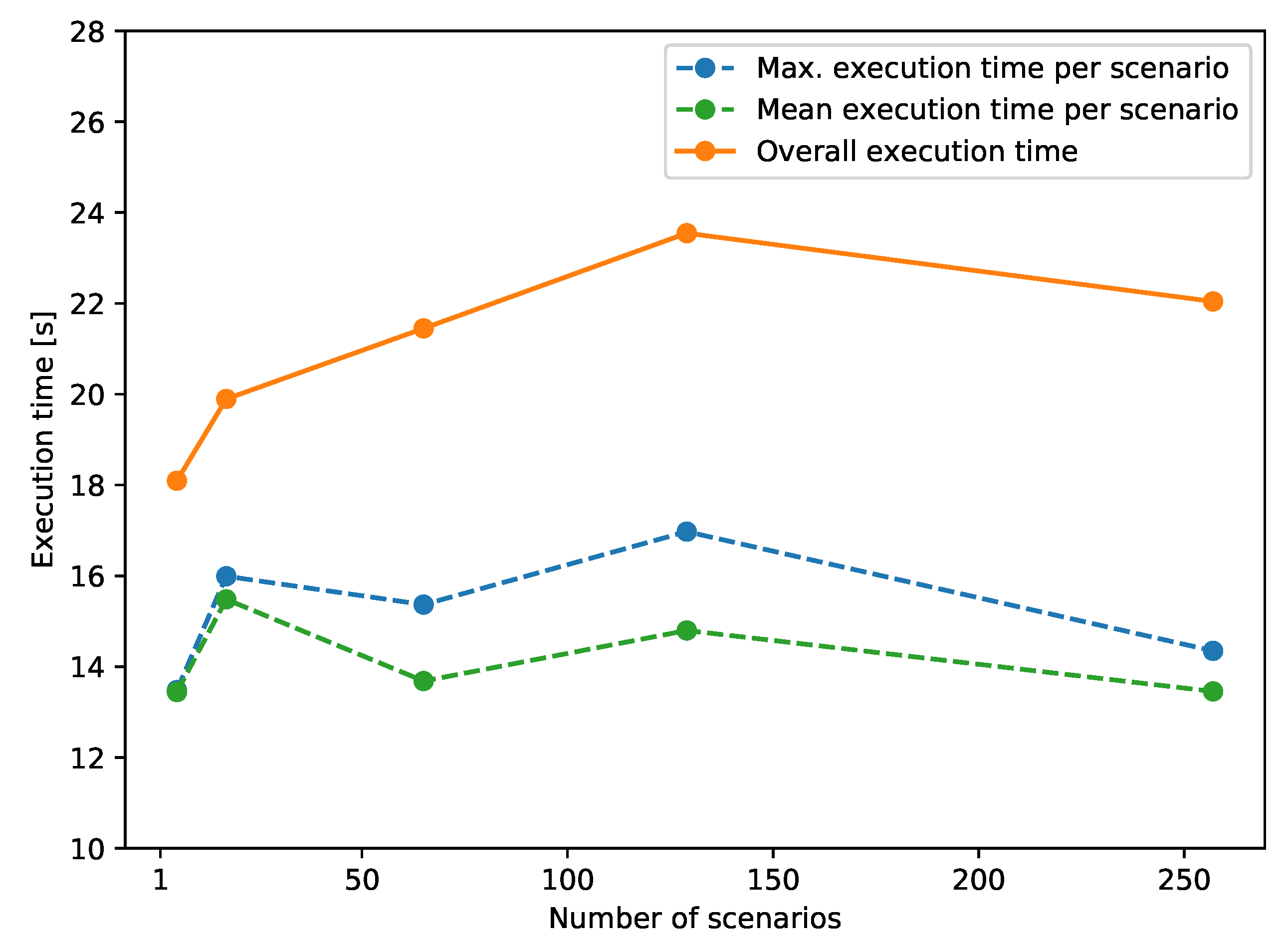
In Figure 5 the solid line shows the overall execution times of the parallel simulation from 4 to 256 scenarios, which are recorded by the execution time of MPI process(es). The dashed lines show the maximum and mean execution time per scenario, which are recorded by the execution time of the simulation executable. It can be noticed that the execution time of the MPI processes remains almost constant regardless of the increasing number of scenarios. Nevertheless, a slight rise in the overall execution time can be observed from the case of 2 to 128 scenarios. Considering the increasing communication overhead with the expanding number of scenarios and the fact that execution time decreases for the case of 256 scenarios, this should be attributed to the varying performance of the application executing on the HPC cluster due to interference from external sources. In fact, it is even expected to have substantial varying execution time for repeated execution of the same program [26]. The interference could come from multiple factors, e.g., operating system jitter, different process-to-node mappings, or contention on shared resources [27,28,29].

Figure 5.
Test case 1 execution time of a parallel simulation with an increasing number of scenarios.
3.2. Test Case 2
To demonstrate the application of the proposed approach on many-scenario simulations, a dynamic contingency simulation is performed on different operating points of the two-area-system grid. We perform an outage event with associated reclosure on each branch by a pair of circuit breaker open and close event, with an interval of . The operating points are generated as follows: For each load in the network, a set of random values is generated following normal distribution:
where is the set of new active power consumption of load i containing 200 data points, and is the original one. Subsequently, for each data point in , the new active power injection of the generators is calculated as:
for 0 3, where and are the original active power injections of the four generators G1 to G4, and as well as are the updated values. and are the total loads in the network before and after the update. is also a random variable which conforms to a uniform distribution . As a result, it generates 2400 different scenarios for the two-area system network with its 12 branches. The simulation configuration is the same as in test case 1 except the simulation duration is reduced to 300 .
The generated scenarios are then simulated with our approach on the HPC cluster. During each execution, eight worker processes are assigned per cluster node. In Figure 6, frequency transients of the generator G1 output from eight scenarios are shown. These scenarios have the same disturbance, transmission line L7to8A trip at time 5 and reclosure at time , based on different operating points. The effects of different operation points to the system transient behavior can be noticed. In these eight scenarios, the system should still be safe considering the largest frequency variation is less than Hz, according to grid codes in ENTSO-E [30] that variations less than 1 Hz is tolerable.
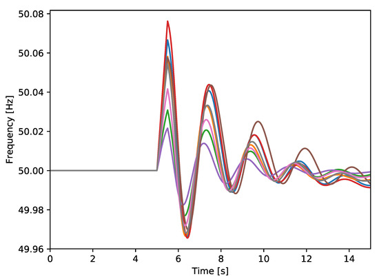
Figure 6.
Frequency transient of generator G1 output for line L7to8A trip and reclosure events based on eight different operating points generated in test case 2.
Based on the execution data of the test case 2, the achieved parallel speedup of our approach with respect to the number of worker processes p is, similarly to the definition in [13], calculated using:
where is the execution time needed for the longest executed worker process of the test case using p processes.
The speedup is calculated for a different number of worker processes used for parallel execution. The results are shown in Figure 7, where for low numbers of processes a linear speedup is established. At this point it must be noted that the simulation execution times for the different scenarios vary strongly: for the shortest and 45 for the longest scenario in case of sequential execution. Hence, for (compared with the number of scenarios) relatively low processor numbers, it can be stated that the implemented dynamic balancing of workloads leads to an efficient parallel execution of the simulation scenarios.
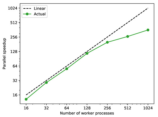
Figure 7.
Parallel speedup against sequential simulation of the 2400 scenarios generated in test case 2 with a different number of worker processes.
For relatively high processor numbers in test case 2, a non-linear parallel speedup can be observed. However, as the execution time of the longest scenario dominates the total execution time with an increasing number of processors more and more, the parallel speedup consideration of the approach is distorted. Therefore, an average worker execution time is defined as:
where is the measured execution time of the i-th worker in case of p parallel processes. Based on this, we define the average speedup as follows:
Obviously, in case all scenarios, for a given p, have the same execution times, the parallel speedup would be equal to the average speedup.
In Figure 8, a nearly linear average speedup with respect to the number of worker processes can be observed. From these results one can deduce that the communication of the task from the manager to the worker processes does not have a considerable effect on the speedup of the approach which is why it scales with the number of processes as expected.
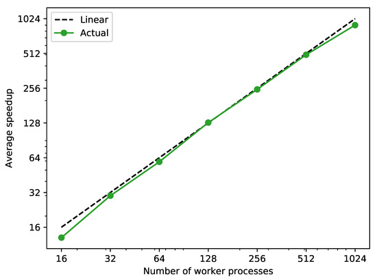
Figure 8.
Average speedup against sequential simulation of the 2400 scenarios generated in test case 2 with a different number of worker processes.
3.3. Test Case 3
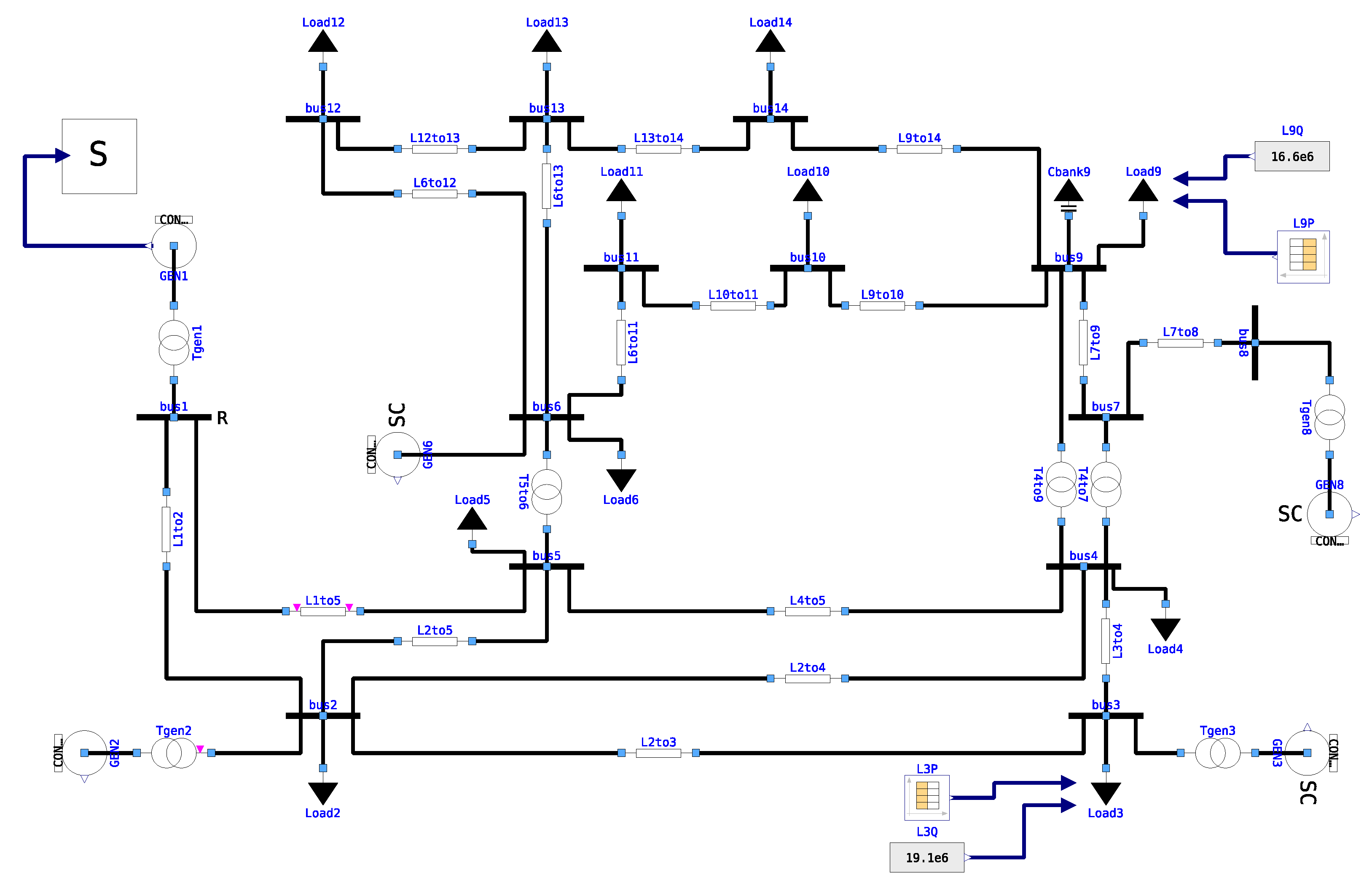
To demonstrate the approach with a more standardized and larger electric network model, similar benchmarks as in Section 3.1 is performed on the IEEE 14-bus system [23]. The Modelica model of the system, as shown in Figure 9, is provided by the PowerGrids library [17] as an example network, where the static data is obtained from [23] and the dynamic data is added by Réseau de Transport d’Electricité (RTE) based on a classical set of values from large French generation units.
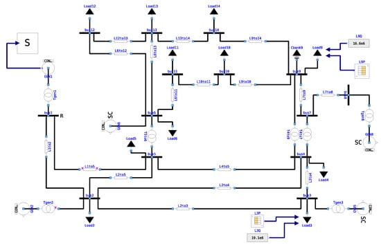
Figure 9.
IEEE 14-bus system implemented using PowerGrids in OpenModelica.
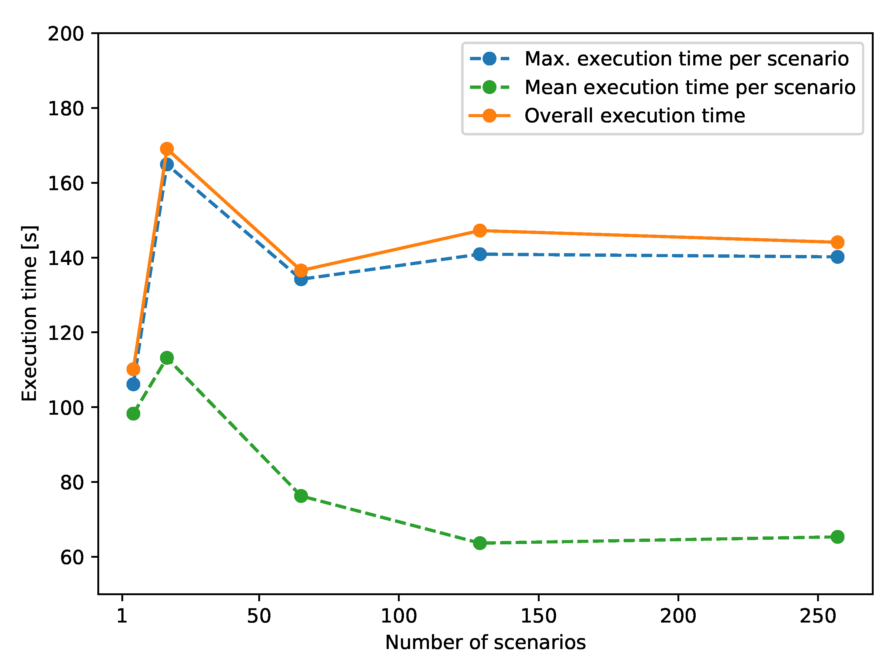
Scenarios for the IEEE 14-bus system are generated similarly as in Section 3.1. Few differences are listed in the following: Firstly, the load steps are added to two loads, Load3 and Load9, instead of only one load as in Section 3.1; secondly, each scenario consists of only one pair of load step events, an increase step of 25% of active power and a decrease step that returns to the nominal value, that occurs at a different point of time. In the end, half of the generated scenarios are load steps on Load3 and the rest are on Load9. The same benchmark as in Section 3.1 is performed, whose result is shown in Figure 10. It can be noticed that, despite the varying execution time per scenario, the overall execution time stays almost constant with the expanding number of scenarios.
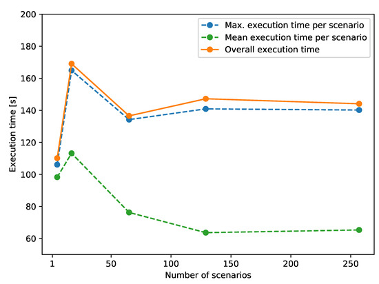
Figure 10.
Test case 3 execution time of a parallel simulation with an increasing number of scenarios.
3.4. Test Case 4
For larger scalability tests, the IEEE 14-bus was duplicated to create 16 system copies in total, with each operating independently in island mode. Furthermore, in one of the system copies, the line L1to5 is removed to create a different operating point. During the simulation, these system copies are connected gradually to form a single connected system. In the end, the resulting 16-copies network consists of 224 buses and 80 generators. Based on these system copies, 10,000 scenarios are created by specifying different connection times and sequences of each system copy.
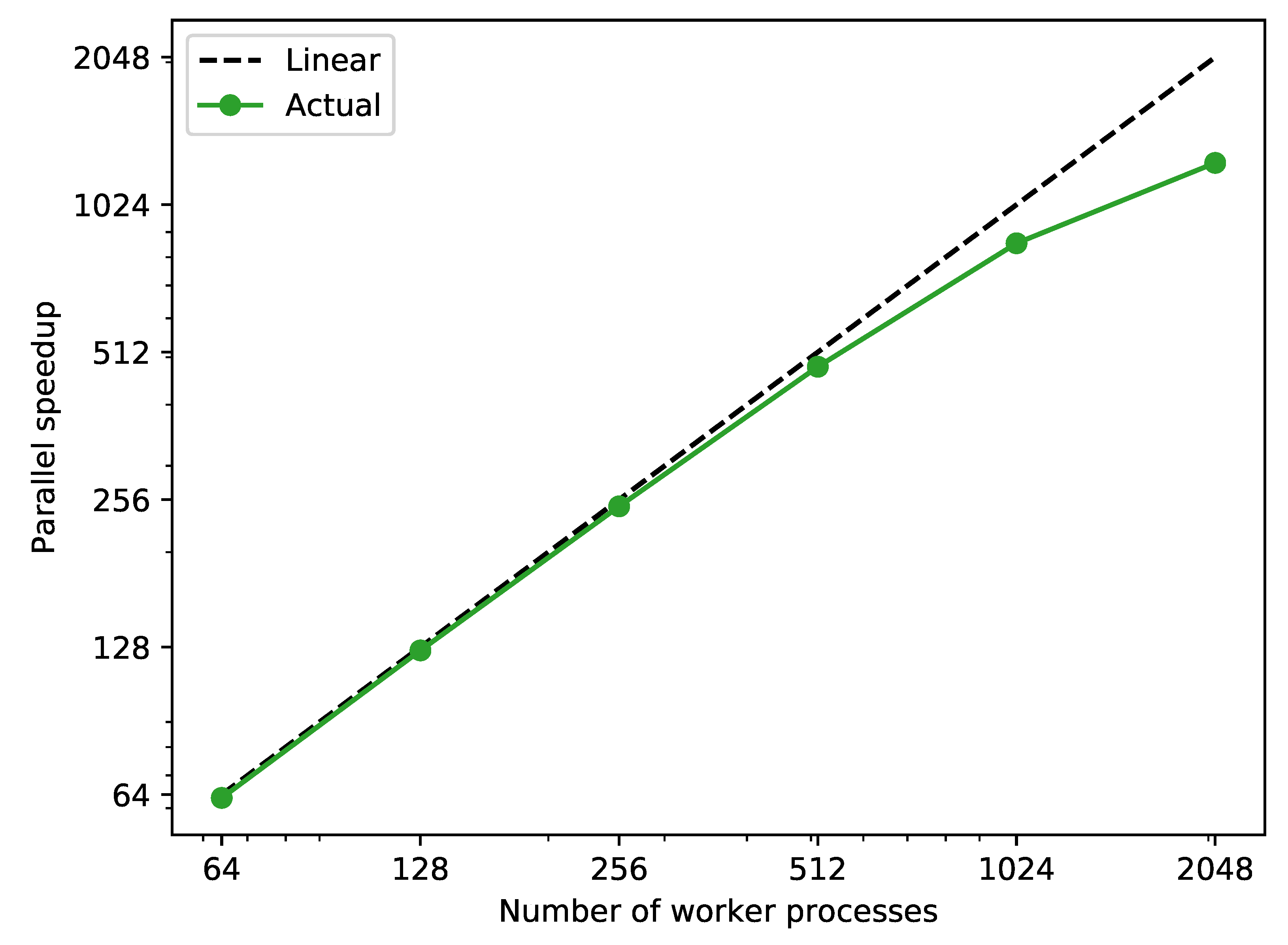
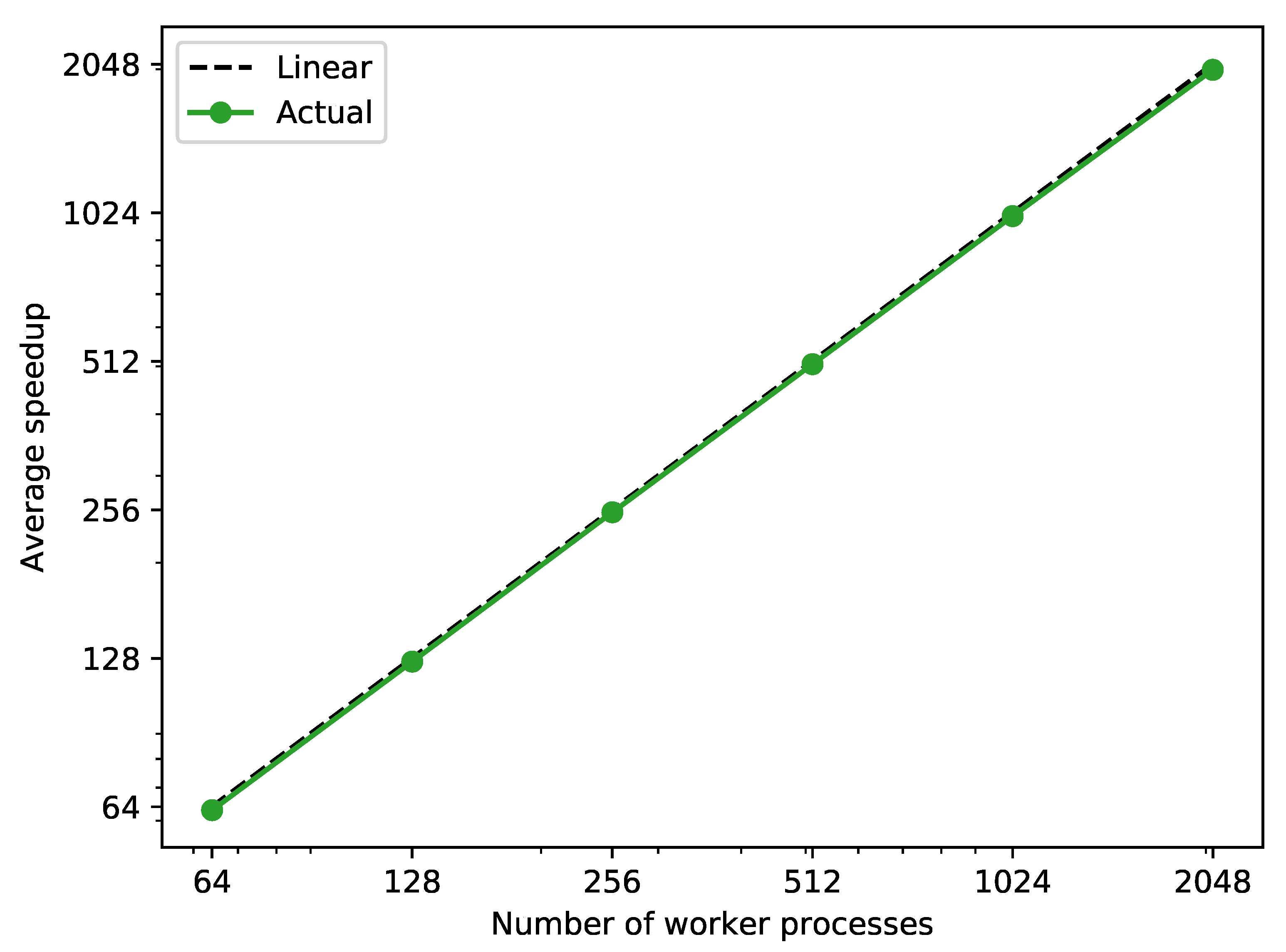
The parallel speed up shown in Figure 11 is calculated by Equation (4), where the sequential execution time is calculated by summing up the execution time of each scenario. Similarly to test case 2, the average speedup shown in Figure 12 is calculated with Equations (5) and (6). It can be noticed that the actual average speedup exhibits a clear linear relationship to the increase of the number of worker processes.
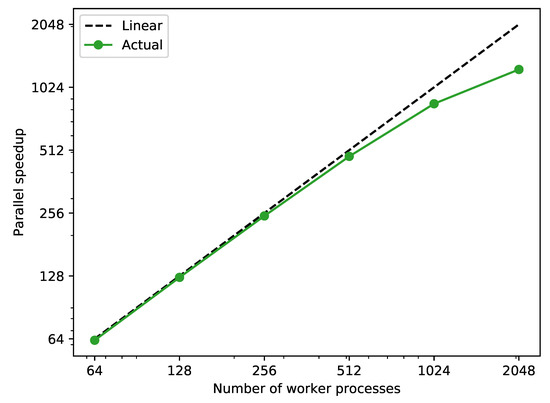
Figure 11.
Parallel speedup against sequential simulation of the 10,000 scenarios generated in test case 4 with a different number of worker processes.
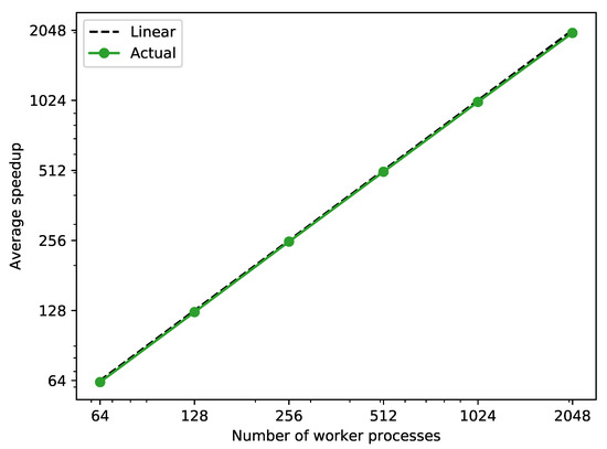
Figure 12.
Average speedup against sequential simulation of the 10,000 scenarios generated in test case 4 with a different number of worker processes.
The sequential simulation would require around 366 to complete, which is around 15 days. However, with the parallel simulation capability provided by our simulation environment, the execution time can be reduced to 15 , with 2048 worker processes.
4. Conclusions and Outlook
This paper introduces our approach to speed up power system studies that need to simulate a large set of scenarios. The approach relies on describing power system models with the object-oriented, equation-based Modelica programming language which is translated to C code and eventually compiled into an executable as well as an MPI- based implementation to parallelize multiple scenario simulations and balance workload among parallel processes. With the aid of MPI to parallelize simulations, the approach can be applied on both inexpensive commodity and highly performance custom clusters. This is realized through our lightweight htcsim module for Python, further utilizing open-source software such as OpenModelica, OMPython, and mpi4py. In addition, the CIM-based power grid data can be used by utilizing CIMverter to translate it to Modelica system models based on a specific Modelica library.
As the benchmark results in Section 3 show, the implemented approach, as open-source software, offers highly parallel scalability. In the second test case, the parallel speedup grows almost linear against the number of processes employed.
Future developments could make use of dynamic scheduling algorithms for parallel tasks [31] to improve the efficiency. Even though the scenario inputs are generated automatically, to automatize the selection of events, including uncertainty consideration, more systematic approach such as event trees [21] can be applied as well.
In the end, the presented approach has wide applicability beyond dynamic contingency analysis. For instance, it can be applied to generate and simulate a large amount of scenarios in order to train artificial intelligence, or be used to compute multiple power system simulations generated in the middle of an optimization algorithm, e.g., a genetic algorithm or an optimal power flow algorithm considering dynamics, etc. such that the overall simulation time can be significantly reduced.
This approach could readily support any non-intrusive uncertainty quantification approach as well, e.g., Monte Carlo, collocation, non-intrusive polynomial chaos, as long as the input scenarios are properly defined. As an example, for a given scenario a certain probability density function (PDF) for some of the components, e.g., load, generation unit, can be defined. Samples are then generated and a Monte Carlo simulation is executed. It is clear that the cases, i.e., the power system simulations to be executed for the Monte Carlo simulation, are very high. That could also be an example of application to be addressed by our approach.
In case of complex scenario branching that leads to a dramatic expansion of the scenario space. Our approach could thus be extended in a way that the worker informs the master about additional scenarios to be executed. The master could then delegate them to the workers.
Cloud computing has not been mentioned as the presented approach is not a so-called cloud-native solution. This means that it is restricted to MPI which was not designed for a dynamic cloud environment. However, since cloud computing, usually at Infrastructure as a Service (IaaS) level, can provide the computational resources for HPC with MPI implementation and all other requirements, our approach can also leverage cloud computing environments.
Author Contributions
Conceptualization, methodology, investigation, and resources, J.Z., L.R., S.H.J., S.D., and A.B.; software and visualization, J.Z. and L.R.; validation, J.Z. and S.H.J.; data curation, J.Z.; writing—original draft preparation, J.Z., L.R., and S.H.J.; writing—review and editing, S.D. and A.B.; supervision and project administration, L.R., S.D., and A.B.; funding acquisition, S.D. and A.B. All authors have read and agreed to the published version of the manuscript.
Funding
The work of J.Z., L.R. and A.B. is supported by the Helmholtz Association under the Joint Initiative Energy Systems Integration. The work of S. D’Arco and S. Jakobsen is supported by the project SynchroPhasor-based Automatic Real-time Control (SPARC), funded by the ENERGIX Program of the Research Council of Norway, under project 280967, and industry partners, Statnett, Fingrid, Energinet, Svenska Kraftnät, Landsnet, and General Electric (GE).
Data Availability Statement
The data presented in this study is available on request from the corresponding author. The data are not publicly available due to unpublished results in this project.
Acknowledgments
We thank the Jülich Supercomputing Centre for the provision of the JURECA supercomputer and the kind assistance.
Conflicts of Interest
The authors declare no conflict of interest.
Abbreviations
The following abbreviations are used in this manuscript:
| AI | artificial intelligence |
| AST | abstract syntax tree |
| CIM | Common Information Model |
| CGMES | Common Grid Model Exchange Standard |
| DSA | dynamic security assessment |
| DSL | domain specific language |
| DAE | differential-algebraic system of equations |
| DP | dynamic phasor |
| IaaS | Infrastructure as a Service |
| SP | static phasor |
| EMT | electro-magnetic transient |
| HPC | high-performance computing |
| MPI | message-passing interface |
| OMC | OpenModelica Compiler |
| PMU | phasor measurement unit |
| probability density function | |
| RTE | Réseau de Transport d’Electricité |
| SCADA | supervisory control and data acquisition |
| SPMD | single program, multiple data |
| TSO | transmission system operator |
| XML | extensible markup language |
References
- Mitra, P.; Vittal, V.; Keel, B.; Mistry, J. A Systematic Approach to n-1-1 Analysis for Power System Security Assessment. IEEE Power Energy Technol. Syst. J. 2016, 3, 71–80. [Google Scholar] [CrossRef]
- Varela, B.J.; Hatziargyriou, N.; Puglisi, L.J. The IGREENGrid Project- Increasing Hosting Capacity in Distribution Grids. IEEE Power Energy Mag. 2017, 15, 30–40. [Google Scholar] [CrossRef]
- Evangelopoulos, V.A.; Georgilakis, P.S.; Hatziargyriou, N.D. Optimal operation of smart distribution networks: A review of models, methods and future research. Electr. Power Syst. Res. 2016, 140, 95–106. [Google Scholar] [CrossRef]
- Cheng, L.; Yu, T. A new generation of AI: A review and perspective on machine learning technologies applied to smart energy and electric power systems. Int. J. Energy Res. 2019, 43, 1928–1973. [Google Scholar] [CrossRef]
- Khaitan, S.K. A survey of high-performance computing approaches in power systems. In Proceedings of the 2016 IEEE Power and Energy Society General Meeting (PESGM), Boston, MA, USA, 17–21 July 2016. [Google Scholar] [CrossRef]
- Liu, Y.; Liang, S.; He, C.; Zhou, Z.; Fang, W.; Li, Y.; Wang, Y. A Cloud-computing and big data based wide area monitoring of power grids strategy. In IOP Conference Series: Materials Science and Engineering; IOP Publishing Ltd.: Bristol, UK, 2019; Volume 677. [Google Scholar]
- SIGUARD DSA—Transmission System Stability and Dynamic Security Assessment. Available online: https://new.siemens.com/global/en/products/energy/energy-automation-and-smart-grid/grid-resiliency-software/siguard-dsa.html (accessed on 10 November 2020).
- DSA Tools-Dynamic Security Assessment Software. Available online: https://www.dsatools.com/ (accessed on 10 November 2020).
- Khan, S.; Latif, A. Python based scenario design and parallel simulation method for transient rotor angle stability assessment in PowerFactory. In Proceedings of the 2019 IEEE Milan PowerTech, Milan, Italy, 23–27 June 2019; pp. 1–6. [Google Scholar]
- Vyakaranam, B.G.; Samaan, N.A.; Li, X.; Huang, R.; Chen, Y.; Vallem, M.R.; Nguyen, T.B.; Tbaileh, A.; Elizondo, M.A.; Fan, X.; et al. Dynamic Contingency Analysis Tool 2.0 User Manual with Test System Examples; Pacific Northwest National Lab.: Richland, WA, USA, 2019. [Google Scholar]
- Chen, Y.; Glaesemann, K.; Li, X.; Palmer, B.; Huang, R.; Vyakaranam, B. A Generic Advanced Computing Framework for Executing Windows-based Dynamic Contingency Analysis Tool in Parallel on Cluster Machines. In Proceedings of the 2020 IEEE Power Energy Society General Meeting (PESGM), Montreal, QC, Canada, 2–6 August 2020; pp. 1–5. [Google Scholar]
- Khaitan, S.K.; McCalley, J.D. Dynamic Load Balancing and Scheduling for Parallel Power System Dynamic Contingency Analysis. In High Performance Computing in Power and Energy Systems; Khaitan, S.K., Gupta, A., Eds.; Springer: Berlin/Heidelberg, Germany, 2013; pp. 189–209. [Google Scholar]
- Quinn, M.J. Parallel Programming in C with MPI and OpenMP; McGraw-Hill Education Group: New York, NY, USA, 2003. [Google Scholar]
- Razik, L.; Dinkelbach, J.; Mirz, M.; Monti, A. CIMverter—A template-based flexibly extensible open-source converter from CIM to Modelica. Energy Inform. 2018, 1, 195–212. [Google Scholar] [CrossRef]
- Fritzson, P. Principles of Object Oriented Modeling and Simulation with Modelica 3.3; John Wiley & Sons, Inc.: Hoboken, NJ, USA, 2014. [Google Scholar]
- Mirz, M.; Netze, L.; Monti, A. A multi-level approach to power system modelica models. In Proceedings of the 2016 IEEE 17th Workshop on Control and Modeling for Power Electronics (COMPEL), Trondheim, Norway, 27–30 June 2016; pp. 1–7. [Google Scholar]
- Bartolini, A.; Casella, F.; Guironnet, A. Towards Pan-European Power Grid Modelling in Modelica: Design Principles and a Prototype for a Reference Power System Library. In Proceedings of the 13th International Modelica Conference, Regensburg, Germany, 4–6 March 2019; Linköping University Electronic Press: Linköping, Sweden, 2019. [Google Scholar]
- Franke, R.; Wiesmann, H. Flexible modeling of electrical power systems–the Modelica PowerSystems library. In Proceedings of the 10th International Modelica Conference, Lund, Sweden, 10–12 March 2014; Linköping University Electronic Press: Linköping, Sweden, 2014. [Google Scholar]
- Dalcín, L.; Paz, R.; Storti, M.; D’Elía, J. MPI for Python: Performance improvements and MPI-2 extensions. J. Parallel Distrib. Comput. 2008, 68, 655–662. [Google Scholar] [CrossRef]
- Sielemann, M.; Casella, F.; Otter, M.; Clauß, C.; Eborn, J.; Matsson, S.E.; Olsson, H. Robust initialization of differential-algebraic equations using homotopy. In Proceedings of the 8th International Modelica Conference, Dresden, Germany, 20–22 March 2011; Linköping University Electronic Press: Linköping, Sweden, 2011; pp. 75–85. [Google Scholar]
- Solvang, E.H.; Sperstad, I.B.; Jakobsen, S.H.; Uhlen, K. Dynamic simulation of simultaneous HVDC contingencies relevant for vulnerability assessment of the nordic power system. In Proceedings of the 2019 IEEE Milan PowerTech, Milan, Italy, 23–27 June 2019; pp. 1–6. [Google Scholar]
- Kundur, P. Power System Stability and Control; McGraw-Hill Education: New York, NY, USA, 1994. [Google Scholar]
- 14 Bus Power Flow Test Case. Available online: http://labs.ece.uw.edu/pstca/pf14/pg_tca14bus.htm (accessed on 16 April 2021).
- Razik, L.; Schumacher, L.; Monti, A.; Guironnet, A.; Bureau, G. A comparative analysis of LU decomposition methods for power system simulations. In Proceedings of the 2019 IEEE Milan PowerTech, Milan, Italy, 23–27 June 2019; pp. 1–6. [Google Scholar]
- Hindmarsh, A.C.; Brown, P.N.; Grant, K.E.; Lee, S.L.; Serban, R.; Shumaker, D.E.; Woodward, C.S. SUNDIALS: Suite of Nonlinear and Differential/Algebraic Equation Solvers. ACM Trans. Math. Softw. 2005, 31, 363–396. [Google Scholar] [CrossRef]
- Nogueira, P.E.; Matias, R.; Vicente, E. An experimental study on execution time variation in computer experiments. In Proceedings of the ACM Symposium on Applied Computing, Gyeongju, Korea, 24–28 March 2014; pp. 1529–1534. [Google Scholar]
- Tsafrir, D.; Etsion, Y.; Feitelson, D.G.; Kirkpatrick, S. System noise, OS clock ticks, and fine-grained parallel applications. In Proceedings of the 19th Annual International Conference on Supercomputing, Cambridge, MA, USA, 20–22 June 2005; pp. 303–312. [Google Scholar]
- Kuo, C.S.; Shah, A.; Nomura, A.; Matsuoka, S.; Wolf, F. How file access patterns influence interference among cluster applications. In Proceedings of the 2014 IEEE International Conference on Cluster Computing (CLUSTER), Madrid, Spain, 22–26 September 2014; pp. 185–193. [Google Scholar]
- Shah, A.; Müller, M.; Wolf, F. Estimating the Impact of External Interference on Application Performance. In Euro-Par 2018: Parallel Processing, Proceedings of the 24th International Conference on Parallel and Distributed Computing, Turin, Italy, 27–31 August 2018; Lecture Notes in Computer Science (Including Subseries Lecture Notes in Artificial Intelligence and Lecture Notes in Bioinformatics); Springer: Berlin/Heidelberg, Germany, 2018; Volume 11014, pp. 46–58. [Google Scholar]
- ENTSO-E. Commission Regulation (EU) 2016/631 of 14 April 2016 establishing a network code on requirements for grid connection of generators. Official Journal of the European Union, 27 April 2016; 1–68. [Google Scholar]
- Barbosa, J.G.; Moreira, B. Dynamic scheduling of a batch of parallel task jobs on heterogeneous clusters. Parallel Comput. 2011, 37, 428–438. [Google Scholar] [CrossRef]


Publisher’s Note: MDPI stays neutral with regard to jurisdictional claims in published maps and institutional affiliations. |
© 2021 by the authors. Licensee MDPI, Basel, Switzerland. This article is an open access article distributed under the terms and conditions of the Creative Commons Attribution (CC BY) license (https://creativecommons.org/licenses/by/4.0/).