Abstract
In this paper, a novel control algorithm with the capacity of fault tolerance and anti-disturbance is discussed for the systems subjected to actuator faults and mismatched disturbances. The fault diagnosis observer (FDO) and the disturbance observer (DO) are successively designed to estimate the dynamics of unknown faults and disturbances. Furthermore, with the help of the observed information, a sliding surface and the corresponding sliding mode controller are proposed to compensate the actuator faults and eliminate the impact of mismatched disturbances simultaneously. Meanwhile, the convex optimization algorithm is discussed to guarantee the stability of the controlled system. The favorable anti-disturbance and fault-tolerant results can also be proved. Finally, the validity of the algorithm is certified by the simulation results for typical unmanned aerial vehicles (UAV) systems.
1. Introduction
It is well known that nearly all control systems are affected by disturbances or uncertainties, which makes it difficult to accurately analyze and control them [1]. Most cases even lead to a prominent drop in the dynamical performance of the system. Therefore, it is very important to discuss effective anti-disturbance control algorithms. In past literature, a large quantity of remarkable control methods, such as / control [2,3], active disturbance rejection control (ADRC) [4,5], output regulator theory [6], back-stepping control [7] and robust control [8], have received significant attention in the field of control theory. However, most existing results only relate to the disturbance attenuation problem and cannot directly compensate unknown disturbances [9]. Based on this, disturbance observer-based control (DOBC), as a popular active anti-disturbance method, has been applied in many engineering practices [10,11,12]. The merit of the DOBC method is that the baseline controller can retain the nominal performance without changing its configuration [13]. The suppression of matching disturbances can be effectively handled by the design of a feedback controller which is based on disturbance observers. However, in practical applications, not every disturbance or uncertainty of the controlled system can strictly meet the matching conditions [14]. For the processing of mismatching disturbances, sliding mode control (SMC) is an effective robust control method. The SMC method is recognized as a powerful methodology, which can manage compensations to disturbances and faults in control systems [15,16,17,18]. To date, lots of SMC methods have been studied, such as adaptive SMC methods [19], terminal SMC methods [20] and integral SMC methods [21]. The authors of [22] proposed an SMC method based on a disturbance observer (DO) for uncertain systems with mismatched disturbances. In [23], SMC based on nonlinear DO is designed to suppress mismatched disturbances and reduce chattering. Recently, there have been some novel results related to sliding mode control of second-order systems. In [24], by designing an extended multiple sliding surface, an effective algorithm is proposed for a system with matched/unmatched uncertainties. For further improving the robustness, [25] addresses a dynamic SMC theory for over-actuated autonomous underwater vehicle (AUV) systems. In [26], a robust SMC method is considered to ensure stability and better performance of a hovering AUV subject to model uncertainties and ocean current disturbance. These proposed SMC methods have potential value in dealing with those uncertain parameters and disturbances that exist in controlled systems.
In the industrial information society, faults of any link in the complex control system will cause immeasurable losses to the entire system [27]. At the same time, it is difficult to monitor the faults in real time, which will increase the operating cost of the control system and reduce the operating efficiency of the system [28]. Therefore, fault diagnosis (FD) and fault-tolerant control (FTC) technologies are proposed to reduce the various impacts caused by faults and maintain the stable operation of the system. Since scholars realized the practical application value of FD and FTC, theoretical research has been developed and fruitful results have been obtained [29,30,31,32,33,34,35,36]. In [29], a spacecraft attitude tracking control method based on a new adaptive integral terminal sliding mode fault-tolerant control strategy was studied. In consideration of actuator failure, external disturbances and actuator saturation, it can ensure the stable tracking performance of the spacecraft’s attitude. The authors of [33] analyzed a constrained control scheme based on model-referenced adaptive control. The model considered the longitudinal motion of a commercial aircraft with additive and multiplicative faults and saturated nonlinearity. Many studies assume that the fault information is known. In fact, the fault information is not known in the actual system. Therefore, a fault diagnosis observer (FDO) is proposed to effectively identify faults, which is beneficial to the design of fault-tolerant controllers. The authors of [37] designed a sliding mode observer to estimate faults for nonlinear uncertain systems. The authors of [38] gave an LMI design method for a new type of unknown input observer that can handle noise and uncertainty at the same time. FTC technology can be divided into active FTC and passive FTC [39]. The control method adopted by passive FTC does not depend on the FD system, and the stability of the system is guaranteed by establishing a fixed fault-tolerant controller. Active FTC is a series of control adjustment strategies adopted after the FD system obtains the fault status.
In real applications, it is worthwhile to point out that both disturbances and faults may influence the system performance simultaneously. In fact, this problem has also been studied. Some results only realize the estimation of the faults which have not been compensated effectively [40,41]. Meanwhile, many approaches are used to reject disturbances or uncertainties by feedback control rather than feedforward compensation control [42,43]. More importantly, most results merely relate to the inputs, actuator faults and disturbances which are constrained in the same channel [44,45]. In this case, it is difficult to judge whether the indescribable performance is caused by disturbances or faults. Hence, when the system is simultaneously confronted with faults and disturbances, how to distinguish them is the first problem. In addition, compared with those matched results, the mismatched conditions will also become more challenging in the aspect of controller design and performance analysis.
Motived by the above analysis, a novel composite observer including FDO and DO is designed to dynamically reject unknown faults and mismatched disturbances. To make up for the mismatched disturbances, a sliding surface and a sliding mode controller are established, which not only compensate the faults and disturbances simultaneously but also guarantee the ultimately uniformly bounded (UUB) performance of a controlled system. A flow chart is shown in Figure 1. It can be seen that the proposed algorithm can realize the unmatched dynamical compensation, which improves matched results and the traditional robust problem. In addition, compared with some single anti-disturbance or fault-tolerance algorithms [46,47], the result also represents a quite significant extension. Finally, as for a typical unmanned aerial vehicle (UAV) system, a simulation example is given to certify the validity of the algorithm.
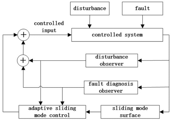
Figure 1.
Anti-disturbance fault-tolerant sliding mode control.
Notation: For a matrix O, is expressed as ; I and 0, respectively, denote identity matrix and zero matrix. If there is no description, matrices are supposed to have compatible dimensions.
2. System Description
Consider a system with actuator faults and unknown disturbances, as follows:
where , , , and , respectively, stand for the system state, the control input, the actuator faults, the exogenous disturbances and the control input. A, , , C are coefficient matrices.
Obviously, the disturbance and the control input enter the system from different channels, thus forming a mismatched disturbance. It was also mentioned in [14] that the existing DOBC does not work against this disturbance.
Assumption A1.
The pair is controllable, and matrices and are full columns.
Assumption A2.
The unknown fault and the mismatched disturbance , respectively, satisfy and , where and .
3. Composite Observer Design
For the sake of estimating the actuator faults and the mismatched disturbances, FDO and DO are shown in this section.
3.1. FDO Design
The following FDO is set up to complete the fault estimation:
where and are estimations of and , respectively. is the FDO gain to be solved later. is a designed auxiliary variable.
Defining and , the fault estimation error system can be expressed as
In this subsection, an FDO is designed for fault estimation. In the following subsection, we construct a DO so that the mismatched disturbances can be estimated accurately.
3.2. DO Design
The unknown mismatched disturbance is supposed to be constructed by an exogenous system as
where is the disturbance vector, W and V are known coefficient matrices.
should be estimated to identify the mismatched disturbance . According to the state observer programming approach, (4) is able to be re-expressed as
where is the equivalent output. Then, error is defined, and the effect of is to enhance the estimation precision, where . Next, can be set up by the Luenberger observer structure as
In order to remove in , by introducing into , DO can be established as
where is the estimation of , is DO gain to be solved later and is an auxiliary variable, which can be described as
Defining , the disturbance estimation error system can be obtained from – as
In this subsection, a DO is designed for disturbance estimation. In the next subsection, we determine the FDO gain and DO gain to make the fault estimation error and the disturbance estimation error converge to zero.
3.3. Performance Analysis of Error System
By defining and combining estimation error Equations and , we have
Assumption A3.
For the observers of actuator faults and mismatched faults , and , respectively, satisfy and , where and are positive scalars.
Next, the following theorems can be obtained by the design of the observers above.
Theorem 1.
For known parameters and , if there exist matrices , satisfying the following LMI
where the fault diagnosis observer gain can be solved by , then the fault estimation error system is UUB.
Proof.
A Lyapunov function is selected as
Under the fault estimation error system , one has
Based on a Schur complement formula and LMI , we can obtain . Next, (13) can be rewritten as
where . It is easy to deduce that , which means that is UUB. □
Theorem 2.
For a known parameter , if there exist matrices , satisfying the following LMI
where the disturbance observer gain can be solved by , then the disturbance estimation error system is UUB.
Proof.
A Lyapunov function is selected as
According to the disturbance estimation error system , we can obtain
Based on a Schur complement formula and LMI , we can obtain . Next, (17) can be rewritten as
where . It is easy to deduce that , which means that is UUB. □
In the next section, a sliding surface and a sliding mode controller are designed to composite the actuator faults and mismatched disturbances simultaneously to ensure the system stability.
4. Controller Design and Dynamical Performance Analysis
A sliding surface is selected as
where can be determined later.
Now, state can be guaranteed to be UBB and finally reach the sliding surface .
Theorem 3.
The system state in is UBB when the matrix is the solution of matrix inequality
where parameters and can be determined later.
Proof.
A Lyapunov function is selected as
According to the system , we can obtain
where and . If there is a matrix that satisfies the inequality , it is easy to find that the system state is UUB. □
In this study, it can be guaranteed that the mismatched DO error is finite, but we may not be able to obtain its specific upper limit. Therefore, it is necessary to put forward adaptive SMC to deal with this issue. Adaptive SMC can meet the reachability condition of , as shown below:
where and the adaptive law is selected as
where h is a positive parameter which can be designed.
Theorem 4.
For the designed sliding surface (19), it can be ensured that the state of system can finally reach the designed sliding surface.
Proof.
is defined and the Lyapunov function is selected as
then we take the time derivative of (25), and then it can be found that -4.6cm0cm
where is a positive variable. can be guaranteed by (26). This means that the reachability condition of SMC can be met. □
5. Numerical Illustrations
In this section, we take the UAV’s longitudinal motion equations into consideration. A four-state one-input longitudinal model can be shown as
where the state variables, respectively, stand for total velocity V , angle of attack , pitch rate q and pitch angle . Note that the notion should be the dimensionless number of q, which can be expressed by . Thrust T and elevator deflection angle are control variables. Furthermore, the dynamic pressure can be described as . All related parameters are displayed in Table 1.

Table 1.
Parameters in (25).
The linearization UAV systems which are subject to actuator faults and mismatched disturbances can be described by
where
The initial conditions of the state are defined as , , and .
In the following section, we consider FDO and DO for different conditions.
Model 1: The actuator fault is supposed to occur at the 15th second as
and the mismatched disturbances can be described as with
Meanwhile, by defining the parameters , , , and solving inequations , , , the control gains , , the FDO gain and the DO gain are found to be
where the sliding surface gain is calculated as
The initial values of states are assumed as . Figure 2 and Figure 3, respectively, display the dynamic trajectories of constant fault and attenuated harmonic disturbance, as well as their accurate estimates. It can be concluded that the designed FO and DO show effective estimation performances. The dynamic trajectory of the sliding surface is shown in Figure 4, and it can be proved that the sliding surface is reachable. Figure 5 and Figure 6, respectively, show the thrust and the elevator deflection angle of a UAV system that vary with time, which also imply that the UAV system is eventually stable.
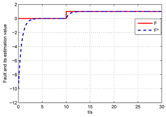
Figure 2.
Fault and its estimation value in model 1.
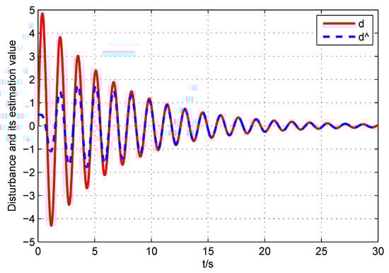
Figure 3.
Disturbance and its estimation value in model 1.
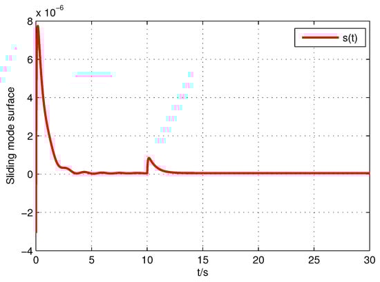
Figure 4.
The sliding mode surface in model 1.
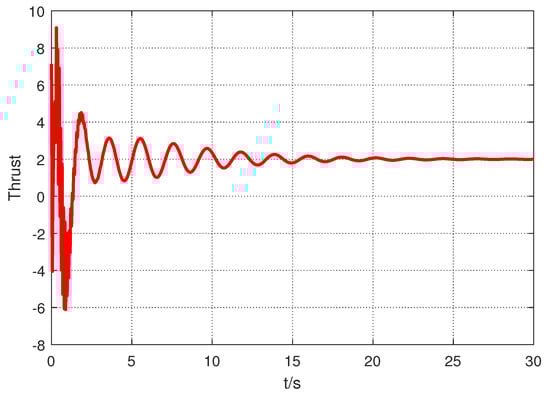
Figure 5.
Thrust of UAV system in model 1.
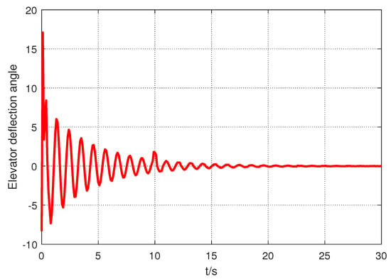
Figure 6.
Elevator deflection angle of UAV system in model 1.
Model 2: The second kind of the actuator fault is supposed to occur at the 15th second as
and the mismatched disturbances can be described as in with
At the same time, by defining the parameters , , , and solving inequations , , , the control gains , , the FDO gain and the DO gain are found to be
where the sliding surface gain is calculated as
The initial values of states are . A favorable fault identification effect is displayed in Figure 7. Meanwhile, from Figure 8, we can find that the mismatched disturbance can be effectively estimated. In addition, the process of system states is shown in Figure 9, which shows that the system states can eventually reach the sliding surface. Figure 10 and Figure 11 show the trajectories of thrust and the elevator deflection angle of the UAV system. The states of the UAV model are designed as in Figure 12, Figure 13, Figure 14 and Figure 15, respectively, which reflect the satisfactory stability performance. It can be seen from the simulation results that the designed anti-disturbance fault-tolerant sliding mode control algorithm is effective.
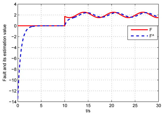
Figure 7.
Fault and its estimation value in model 2.
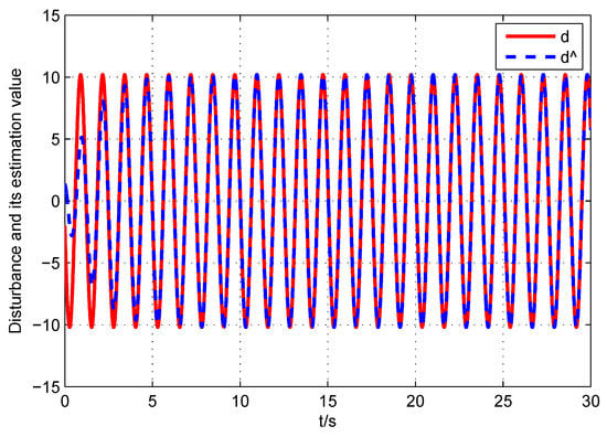
Figure 8.
Disturbance and its estimation value in model 2.
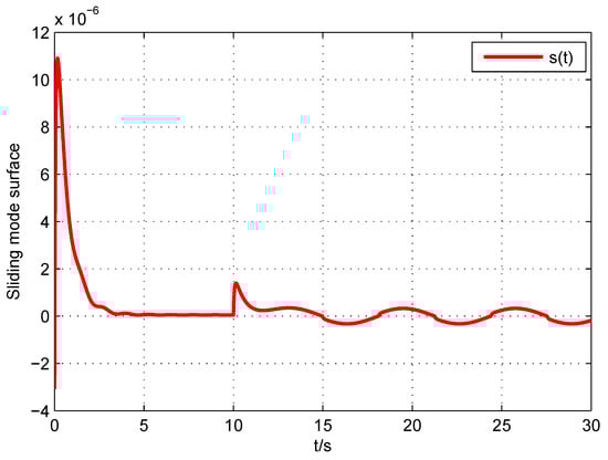
Figure 9.
The sliding mode surface in model 2.
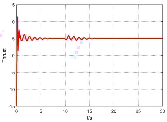
Figure 10.
Thrust of UAV system in model 2.
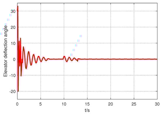
Figure 11.
Elevator deflection angle of UAV system in mode 2.
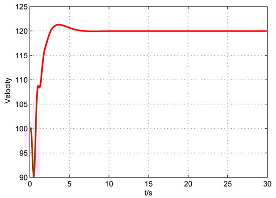
Figure 12.
The velocity of UAV system.
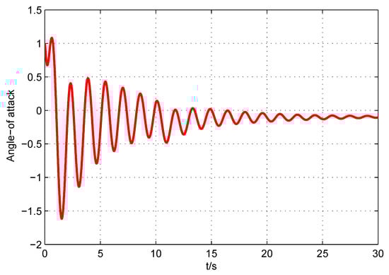
Figure 13.
The angle of attack of UAV system.
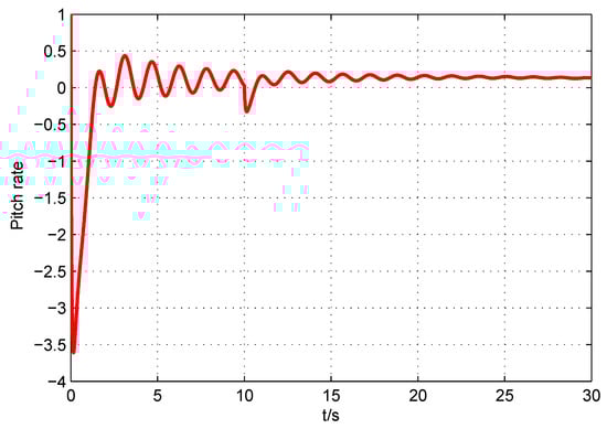
Figure 14.
The pitch rate of UAV system.
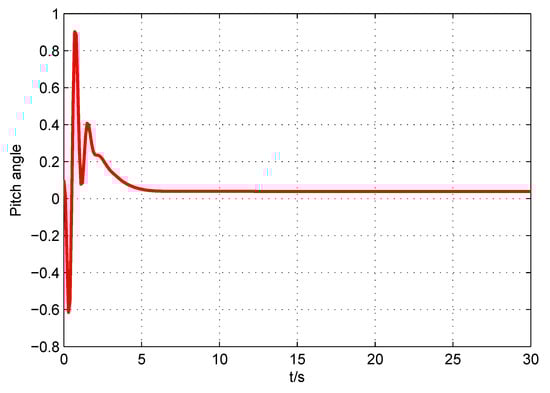
Figure 15.
The pitch angle of UAV system.
6. Conclusions
In this paper, a novel control algorithm with the capacity of fault tolerance and anti-disturbance is put forward for systems subject to unknown faults and mismatched disturbances. In order to distinguish the effects of the faults and disturbances, FDO and DO are designed to estimate the dynamics of unknown faults and disturbances, respectively. With the help of the dynamical estimation results, both a sliding surface and a corresponding sliding mode controller are successively proposed to realize the rejection of the faults and mismatched disturbances. It is noted that the proposed algorithm not only solves the difficulty of unmatched dynamical compensation but also extends single anti-disturbance or fault-tolerance results.
In order to achieve faster convergence, a finite time control problem will be carefully considered as one of our future research topics. Moreover, experimental verification relying on practical equipment will also be discussed in future related work.
Author Contributions
Conceptualization, X.Z. and Z.Z.; Methodology, X.Z. and Y.Y.; Software, X.Z.; writing—original draft preparation, X.Z.; writing—review and editing, Y.Y. All authors have read and agreed to the published version of the manuscript.
Funding
This work is partially supported by the National Natural Science Foundation of China (Grant No. 61973266 and 61803331).
Conflicts of Interest
The authors declare no conflict of interest.
References
- Guo, L.; Cao, S.Y. Anti-disturbance Control for Systems with Multiple Disturbances; CRC Press: Boca Raton, FL, USA, 2013. [Google Scholar]
- Bittar, A.; Sales, R.M. H-2 and H-infinity control for MagLev vehicles. IEEE Control Syst. Mag. 1998, 18, 18–25. [Google Scholar]
- Li, Y.K.; Sun, H.B.; Zong, G.D. Disturbance-observer-based-control and L2-L∞ rsilient control for Markvian jump nonlinear systems with multiple disturbances and its application to single robot arm system. IET Control Theory Appl. 2016, 10, 226–233. [Google Scholar] [CrossRef]
- Gao, Z. Active disturbance rejection control for nonlinear fractionalorder systems. Int. J. Robust Nonlin. Control 2016, 26, 876–892. [Google Scholar] [CrossRef]
- Wu, Z.H.; Guo, B.Z. Approximate decoupling and output tracking for MIMO nonlinear systems with mismatched uncertainties via ADRC approach. J. Franklin Inst. 2018, 355, 3873–3894. [Google Scholar] [CrossRef]
- Isidori, A.; Byrnes, C.I. Output regulation of nonlinear systms. IEEE Trans. Autom. Control 1990, 35, 131–140. [Google Scholar] [CrossRef]
- Morawiec, M. The adaptive backstepping control of permanent magnet synchronous motor supplied by current source inverter. IEEE Trans. Ind. Inf. 2013, 8, 1047–1055. [Google Scholar] [CrossRef]
- Abdel-Rady, Y.; Mohamed, I. Design and implementation of a robust current-control scheme for a PMSM vector drive with a simple adaptive disturbance observer. IEEE Trans. Ind. Electron. 2007, 54, 1981–1988. [Google Scholar]
- Han, J. From PID to active disturbance rejection control. IEEE Trans. Ind. Electron. 2009, 56, 900–906. [Google Scholar] [CrossRef]
- Chen, W.H.; Yang, J.; Zhao, Z.H. Robust control of uncertain nonlinear systems: A nonlinear DOBC approach. J. Dyn. Syst. Meas. Control 2016, 138, 823–828. [Google Scholar] [CrossRef]
- Wang, X.Y.; Li, S.H.; Yu, X.H.; Yang, J. Distributed active anti-disturbance consensus for leader-follower higher-order multi-agent systems with mimatched disturbances. IEEE Trans. Autom. Control 2017, 62, 5795–5801. [Google Scholar] [CrossRef]
- Yang, J.; Cui, H.Y.; Li, S.H.; Zolotas, A. Optimized active disturbance rejection control DC-DC buck converters with uncertainties using a reduced-order GPI observer. IEEE Trans. Circuits Syst. I Reg. Papers 2018, 65, 832–841. [Google Scholar] [CrossRef]
- Liu, C.; Chen, W.H.; Andrews, J. Tracking control of small-scale helicopers using explicit nonlinear MPC augment with disturbance observers. Control Eng. Pract. 2012, 20, 258–268. [Google Scholar] [CrossRef]
- Yang, J.; Su, J.Y.; Li, S.H.; Yu, X.H. High-Order Mismatched Disturbance Compensation for Motion Control Systems Via a Continuous Dynamic Sliding-Mode Approach. IEEE Trans. Ind. Inform. 2014, 10, 604–614. [Google Scholar] [CrossRef]
- Hamayun, M.T.; Edwards, C.; Alwi, H. A fault tolerant control allocation scheme with output integral sliding modes. Automatica 2013, 49, 1830–1837. [Google Scholar] [CrossRef]
- Liu, J.; Vazquez, S.; Wu, L.; Marquez, A.; Gao, H.; Franquelo, L.G. Extended state observer-based sliding -mode control for three-phase power converters. IEEE. Trans. Ind. Election. 2017, 64, 22–31. [Google Scholar] [CrossRef]
- Tapia, A.; Bernal, M.; Fridman, L. Nonlinear sliding mode control design: An LMI approach. Syst. Control Lett. 2017, 104, 38–44. [Google Scholar] [CrossRef]
- Wu, L.; Gao, Y.; Liu, J.; Li, H. Event-triggered sliding mode control of stochastic systems via output feedback. Automatica 2017, 82, 79–92. [Google Scholar] [CrossRef]
- Yang, C.S.; Ni, S.F.; Dai, Y.C.; Huang, X.N.; Zhang, D.D. Anti-disturbance finite-time adaptive sliding mode backstepping control for PV inverter in master-slave-organized islanded microgrid. Energies 2020, 13, 4490. [Google Scholar] [CrossRef]
- Zhu, W.W.; Chen, D.B.; Du, H.B.; Wang, X.Y. Position control for permanent magnet synchronous motor based on neural network and terminal sliding mode control. Trans. Inst. Meas. Control 2020, 42, 1632–1640. [Google Scholar] [CrossRef]
- Lee, J.; Chang, P.H.; Jin, M. Adaptive integral sliding mode control with time-delay estimation for robot manipulators. IEEE Trans. Ind. Electron. 2017, 64, 6796–6804. [Google Scholar] [CrossRef]
- Yang, J.; Li, S.; Yu, X. Sliding mode control for systems with mismatched uncertainties via a disturbance observer. IEEE Trans. Ind. Electron. 2013, 60, 160–169. [Google Scholar] [CrossRef]
- Li, S.; Yang, J.; Chen, W.H. Disturbance Observer-Based Control: Methods and Applications; CRC Press: Boca Raton, FL, USA, 2014. [Google Scholar]
- Thanh, H.L.N.N.; Vu, M.T.; Mung, N.X.; Nguyen, N.P.; Phuong, N.T. Perturbation observer-based robust control using a multiple sliding surfaces for nonlinear systems with influences of matched and unmatched uncertainties. Mathematics 2020, 8, 1371. [Google Scholar] [CrossRef]
- Vu, M.T.; Le, T.-H.; Thanh, H.L.N.N.; Huynh, T.-T.; Van, M.; Hoang, Q.-D.; Do, T.D. Robust position control of an over-actuated underwater vehicle under model uncertainties and ocean current effects using dynamic sliding mode surface and optimal allocation control. Sensors 2021, 21, 747. [Google Scholar] [CrossRef] [PubMed]
- Vu, M.T.; Thanh, H.L.N.N.; Huynh, T.-T.; Duc, T.; Hoang, Q.-D.; Le, T.-H. Station-keeping control of a hovering over-actuated autonomous underwater vehicle under ocean current effects and model uncertainties in horizontal plane. IEEE Access 2021, 9, 6855–6867. [Google Scholar] [CrossRef]
- Du, D.S.; Jiang, B.; Shi, P. Fault Tolerant Control for Control for Switched Linear Systems; Springer: London, UK, 2005. [Google Scholar]
- Blanke, M.; Kinnaert, M.; Lunze, M.; Staroswiecki, M. Diagnosis and Fault-Tolerant Control; Springer: London, UK, 2006. [Google Scholar]
- Li, B.; Hu, Q.; Ma, G.; Yang, Y. Fault Tolerant Attitude Stabilization Incorporating Closed-loop Control Allocation under Actuator Failure. IEEE Trans. Aerosp. Electron. Syst. 2019, 55, 1989–2000. [Google Scholar] [CrossRef]
- Li, L.L.; Luo, H.; Ding, S.X.; Yang, Y.; Peng, K.X. Performance-based fault detection and fault-tolerant control for automatic control systems. Automatica 2019, 99, 308–316. [Google Scholar] [CrossRef]
- Cho, S.; Gao, Z.; Moan, T. Model-based fault detcetion, fault isolation and fault-tolerant control of a blade pitch system in floating wind turbines. Renew. Energy 2018, 120, 306–321. [Google Scholar] [CrossRef]
- Li, Q.; Yuan, J.P.; Sun, C. Robust fault-tolerant saturated control for spacecraft proximity operations with actuator saturations and faults. Adv. Space Res. 2018, 63, 1541–1553. [Google Scholar] [CrossRef]
- Liu, Y.; Dong, X.; Ren, Z.; Cooper, J. Fault-tolerant control for commercial aircraft with actuator faults and constraints. J. Franklin Inst. 2019, 356, 3849–3868. [Google Scholar] [CrossRef]
- Zhang, Y.M.; Guo, L.; Wang, H. Robust filtering for fault tolerant control using output PDFs of non-Gaussian systems. IET Theory Appl. 2007, 1, 636–645. [Google Scholar] [CrossRef]
- Spong, M.W. On the robust control of robot Manipulators. IEEE Trans. Autom. Control 1992, 37, 1782–1786. [Google Scholar] [CrossRef]
- Ducard, G.J. Fault-Tolerant Flight Control and Guidance Systems: Practical Methods for Small Unmanned Aerial Vehicles; Springer: London, UK, 2009. [Google Scholar]
- Wu, Q.; Saif, M. Robust fault diagnosis of a satellite system using a learning strategy and second order sliding mode observer. IEEE Syst. J. 2010, 4, 112–121. [Google Scholar]
- Sharifuddin, M.; Goutam, C.; Kingshook, B. LMI approach to robust unknown input observer design for continuous systems with noise and uncertainties. Int. J. Control Autom. Syst. 2010, 8, 210–219. [Google Scholar]
- Liu, Y.; Yang, G.H. Integrated design of fault estimation and fault-tolerant control for linear multi-agent systems using relative outputs. Neurocomputing 2019, 329, 468–475. [Google Scholar] [CrossRef]
- Du, D.S.; Xu, S.Y.; Cocquempot, V. Actuator fault estimation for discrete-time switched systems with finite-frequency. Syst. Control Lett. 2017, 108, 64–70. [Google Scholar] [CrossRef]
- Xie, X.P.; Yue, D.; Park, J.H. Robust fault estimation design for discrete-time nonliner systems via a modified fuzzy fault estimation observer. ISA Trans. 2018, 73, 22–30. [Google Scholar] [CrossRef]
- Zong, G.; Ren, H.; Karimi, H.R. Event-triggered communication and annular finite-time H∞ filtering for networked switched systems. IEEE Trans. Cybern. 2020, 51, 309–317. [Google Scholar] [CrossRef]
- Yu, P.; Liu, K.-Z.; Wu, M.; She, J. Improved equivalent-input disturbance approach based on H∞ control. IEEE Trans. Ind. Electron. 2020, 67, 8670–8679. [Google Scholar] [CrossRef]
- Rasouli, P.; Moattari, M.; Forouzantabar, A. Nonlinear disturbance observer-based fault-tolerant control for flexible teleoperation systems with actuator constraints and varying time delay. Trans. Inst. Meas. Control 2021, 43, 2246–2257. [Google Scholar] [CrossRef]
- Sun, S.X.; Wei, X.J.; Zhang, H.F.; Karimi, R.R.; Han, H. Composite fault-tolerant control with disturbance observer for stochastic systems with multiple disturbances. J. Fraklin Inst. 2018, 355, 4897–4915. [Google Scholar] [CrossRef]
- Ding, R.Q.; Cheng, M.; Jiang, L.; Hu, G.L. Active fault-tolerant control for electro-hydraulic systems with an independent metering valve against valve faults. IEEE Trans. Ind. Electron. 2021, 68, 7221–7232. [Google Scholar] [CrossRef]
- Xu, J.W.; Yu, X.; Qiao, J.Z. Hybrid disturbance observer-based anti-disturbance composite control with applications to mars landing mission. IEEE Trans. Syst. Man. Cybern. Syst. 2021, 51, 2885–2893. [Google Scholar] [CrossRef]


Publisher’s Note: MDPI stays neutral with regard to jurisdictional claims in published maps and institutional affiliations. |
© 2021 by the authors. Licensee MDPI, Basel, Switzerland. This article is an open access article distributed under the terms and conditions of the Creative Commons Attribution (CC BY) license (https://creativecommons.org/licenses/by/4.0/).