Data-Driven Fault Diagnosis for Satellite Control Moment Gyro Assembly with Multiple In-Phase Faults

Abstract

A satellite can only complete its mission successfully when all its subsystems, including the attitude control subsystem, are in healthy condition and work properly. Control moment gyroscope is a type of actuator used in the attitude control subsystems of satellites. Any fault in the control moment gyroscope can cause the satellite mission failure if it is not detected, isolated, and resolved in time. Fault diagnosis provides an opportunity to detect and isolate the occurring faults and, if accompanied by proactive remedial actions, it can avoid failure and improve the satellite reliability. In this paper, an enhanced data-driven fault diagnosis is introduced for fault isolation of multiple in-phase faults of satellite control moment gyroscopes that has not been addressed in the literature before with high accuracy. The proposed method is based on an optimized support vector machine, and the results yield fault predictions with up to 95.6% accuracy. In addition, a sensitivity analysis with regard to noise, missing values, and missing sensors is done. The results show that the proposed model is robust enough to be used in real applications.

1. Introduction

Satellites are essential assets for space exploration and data collection. Therefore, their fault-free operation is critical, which relies on the health of their subsystems and components. For example, one of the major systems of any satellite is the attitude control subsystem (ACS) that uses different actuators such as reaction wheels, momentum wheels, and control moment gyros (CMGs), among others. If the ACS fails, the satellite cannot complete its mission. Hence, if a fault occurs in any part of the CMGs, it may fail if unattended. Fault isolation can prevent failure and increase satellite reliability by identifying any occurring fault and conducting remedial actions in time. Different fault isolation approaches include the model-based and data-driven categories [1,2,3,4].

The application of different data-driven methods in fault isolation has become popular in recent years. Specifically, different machine learning methods, such as support vector machines (SVM), neural networks, and gradient boosting machines, along with different deep learning methods, are widely used for this application [2,5]. These methods establish a fault isolation scheme by classifying given data to distinguish between different possible faults.

Several research publications cover the fault diagnosis of satellite ACS using SVM, among other data-driven approaches [6,7,8,9]. The SVM is a supervised learning method with reasonable flexibility and can adapt to any application. As each fault scenario can be considered as a class, the SVM can be used for fault diagnosis. In [6], a multi-classifier model is formed based on the Dempster–Shafer theory and SVM, while nonlinear principal component analysis (NPCA) is adopted to reduce the feature size. In [8], SVM and neural networks are used to build a model for the satellite power supply system’s health monitoring. In [7], the combination of random forest (RF), partial least square, SVM, and Naïve Bayes is used to form a framework for detecting and isolating faults. In [9], telemetry data is used as input to extract the features, and principal component analysis (PCA) is used for feature reduction, which is followed by an optimized SVM model using the particle swarm optimization (PSO) method adopted for FDI.

Neural networks (NN) and deep learning methods are also employed for satellite ACS FDI [10,11,12,13]. In [10], Prony analysis is used for feature extraction, and a feed-forward NN is developed for anomaly classification. In [12], first, a model is established to find the characteristics that express the faults using a deep neural network. Next, the fault-to-noise ratio and characteristics differences are amplified using a sliding window. Then, the proposed method is used for fault identification of a satellite ACS. A feed-forward wavelet-based NN is adopted to form an adaptive observer for fault detection. Adopting a feed-forward wavelet-based neural network with a single hidden layer, the proposed method can be applied to nonlinear systems [13]. In [14], Chebyshev Neural Network and genetic algorithm are used to isolate CMG faults using satellite attitude rate data. However, the fault injection in that study does not accommodate in-phase faults, meaning that the faults occur out-of-phase or non-concurrently. That can be a limitation considering that multiple CMGs can become faulty simultaneously. In [15], the authors propose a new third-order nonlinear dynamics for double gimbal control moment gyros (DGCMGs) affected by friction and coupling torques, unmodeled dynamics, or parameter uncertainties that does not directly address the fault isolation and identification challenge and focuses on the dynamics and control of the CMGs under uncertain circumstances.

Various other machine learning approaches such as minimum error minimax probability machine [16], gradient boosting machines (GBM) [17], and kernel principal component analysis [18] are used for fault detection and isolation in aerospace applications.

While several articles exist on ACS fault isolation, most focus on systems that only have one active fault [14]. The proposed models cannot handle cases with multiple in-phase (concurrent) faults, while these cases are likely to occur during a real-life satellite operation. When there is more than one fault present simultaneously, the effect of each fault on the overall system and other subsystem units makes the isolation task more challenging. The only work that has evaluated the multiple in-phase faults [19] reported a maximum accuracy of 66.6%, which is not sufficient for real applications. Thus, there is a need for a specific approach to handle this problem while achieving reasonable accuracy of higher than 90%.

In this work, a new data-driven scheme is developed for fault isolation of multiple in-phase faults on a CMG assembly used in ACS to control a three-axis stabilized satellite in orbit. The proposed method can handle multiple in-phase faults in satellite CMGs to address the shortcomings mentioned above in the literature. Specifically, the fault isolation of multiple concurrent faults with high accuracy. The initial results of this work have been published in [20]. However, the accuracy reported in [20] was low for real-life applications. This paper contains the complete work that has solved the accuracy issue and includes additional insights into the different aspects of the problem, including a comprehensive sensitivity analysis. The challenges faced in addressing this problem include (1) the multiple faults that are active simultaneously, (2) the randomness of the faults inception, duration, and severity, and (3) the fact that the satellite is fully controlled so the effect of faults can be compensated for by the controller and leave the fault isolation scheme blind to the underlying conditions. It is also important to note that (4) the proposed data-driven approach is using satellite level measurements (satellite orientation and angular velocities) to isolate a fault at the actuator level.

The remaining of this paper is organized as follows: In Section 2, the problem at hand is defined. In Section 3, the proposed fault isolation scheme is introduced and described. Section 4 is devoted to the algorithm complexity analysis of the methods used in this paper. In Section 5, a case study is presented to assess the proposed method’s performance. Results are presented and discussed in Section 6. Finally, Section 7 concludes the paper with final remarks and recommendations for future work.

2. Problem Definition

In general, any nonlinear dynamical system can be modeled in state-space as:

$$\Omega :\{\begin{array}{c}{X}_{k+1}=f\left(X_k,u_k,{\theta }_k,{\omega }_k^X\right)\\ {\theta }_{k+1}={\theta }_k+{\omega }_k^{\theta }\\ y_k=g\left(X_k,{\theta }_k\right)+v_k\end{array}$$

(1)

where $X_k\in {ℝ}^n$ is the state vector, $u_k\in {ℝ}^m$ is the control input, ${\theta }_k\in {ℝ}^l$ is the system parameter, $y_k\in {ℝ}^m$ is the measurement, and ${\omega }_k^X,{\omega }_k^{\theta }\in {ℝ}^n$ are the additive process noise for states and parameters, respectively. $v_k\in {ℝ}^m$ is the additive measurement noise, $k$ is the time step of the process, and measurement models are represented by $f(·)$ and $g(·)$, respectively.

Assuming that any change in the physical parameters of the satellite is accompanied by a change in one of the parameters of the system [21], a fault isolation problem can be expressed as:

$${\theta }_k={\theta }_0+{\alpha }_k$$

(2)

where ${\theta }_0\in {ℝ}^L$ is a vector demonstrating the nominal parameter values, ${\alpha }_k\in {ℝ}^L$ is a vector representing the parameter values in the presence of a fault, and $L$ is the number of possible scenarios for faults that can be considered for the satellite. Equation (2) is a demonstration of a multi-parameter model and can be split into $L$ single parameter models as [21]:

$${\Omega }_i:\{{\theta }_k^i={\theta }_0^i+{\alpha }_k^i\hspace{1em}i=1,\dots ,L.$$

(3)

Equation (3) expresses a classification problem with $L$ classes for which a data-driven approach can be used to find a solution. Then, the data-driven method is set to predict the class of the current system state, considering the potential $L$ cases. This can be done once a fault is detected through each fault model shown in (3), where the $i\mathrm{th}$ model captures the $i\mathrm{th}$ system parameter ${\theta }_0^i$ and its severity through ${\alpha }_k^i$. The assumptions made in this work are as follows:

• The induced faults are in phase. Each data instance has assigned fault inception and duration times, which are the same for all CMG units that are faulty.
• The assigned fault severity for each instance is from 0 to 1 to cover all possible fault severities.
• All state measurements are available.
• There is no source of noise nor missing values in the raw input data.

This work aims to design and develop a data-driven fault isolation scheme that can use the system outputs and predict the presence of any possible fault as well as isolate the fault location under the assumptions mentioned above.

3. Proposed Fault Isolation Scheme

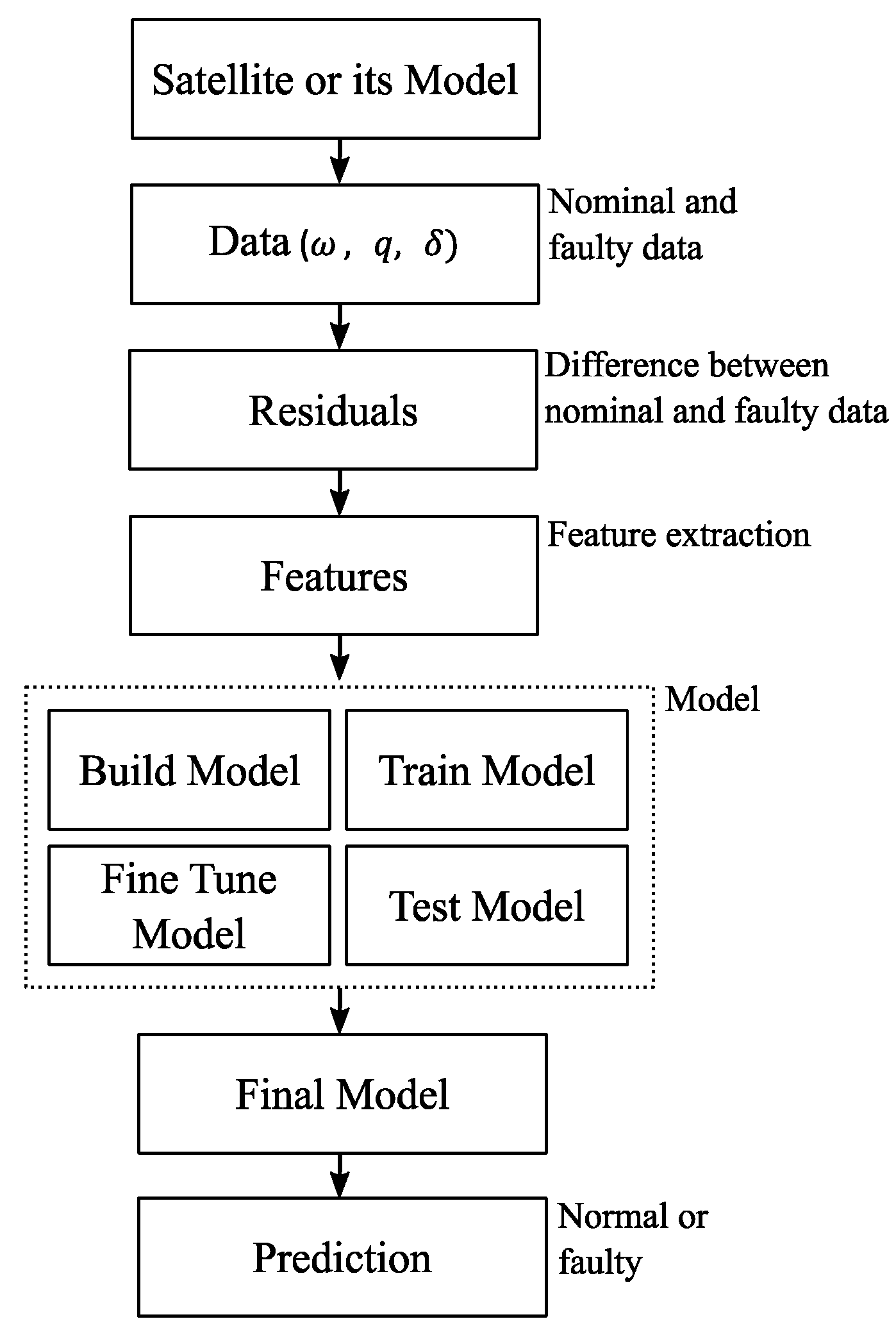
A data-driven fault isolation method is introduced that comprises an optimized machine learning model for isolating multiple in-phase faults of the satellite CMG. First, the features are calculated using the CMG data, and then, feature reduction is made through the PCA. Next, the chosen features are fed to the machine learning model as inputs for the training and testing steps. For improving the performance, the machine learning model is tuned by finding the optimal values of its parameters. Finally, the optimized machine learning model is used for performance evaluation in a case study for isolating multiple in-phase faults of a CMG assembly on a three-axis stabilized satellite in orbit. Figure 1 shows the flow diagram of the proposed fault isolation scheme. As can be seen in Figure 1, the data can be obtained from either a model of the system or the actual physical system. Once data are collected, residuals are generated as the difference between the healthy and faulty unit measurements. Next, essential features are extracted from the residuals that capture the essence of the data for fault isolation. Once features are extracted, model training and tuning start. Once the model is trained, tuned, and tested, the final model is used to evaluate the performance of the proposed scheme in isolating faults in various scenarios. Further details of the proposed scheme are described in Section 3.1, Section 3.2, Section 3.3 and Section 3.4.

3.1. Data Acquisition

The raw data are acquired from a satellite telemetry system or a satellite mathematical model. In this study, a high-fidelity satellite model with four CMG units is used to generate the required data described in Section 5. The raw data comprise satellite attitude quaternions, angular speeds, and the CMGs gimbal angles. The data are stored in a time-series format, with each set representing one of the fault scenarios shown in

Table 1. Different scenarios for faults in the CMG assembly.

Scenario	Faulty CMG(s)	Scenario	Faulty CMG(s)
0	None	8	2, 3
1	1	9	2, 4
2	2	10	3, 4
3	3	11	1, 2, 3
4	4	12	1, 2, 4
5	1, 2	13	1, 3, 4
6	1, 3	14	2, 3, 4
7	1, 4	15	1, 2, 3, 4

. There is a total of 16 scenarios. Scenario 0 represents the system without any fault. Scenarios 1 to 15 represent the system with one, two, three, or four faulty units.

3.2. Data Preprocessing

3.2.1. Residual Calculation

The raw data are used to calculate the residuals. Residuals represent the difference between the system outputs in a nominal and faulty condition. The residuals can be calculated using:

$$r_k^m=y_k^m-y_k^0\hspace{1em}m=0,\dots ,15$$

(4)

where $y^m$ represents the system measurable states/outputs for faulty model $m$, $m$ denotes the desired fault scenario, $y^0$ is the system states/outputs for a healthy model, and $k$ is the measurement time step.

3.2.2. Feature Extraction

The features are extracted from the residual time series. Feature selection/reduction methods are used to reduce the extracted features while looking for the most representative features. There are various methods for feature extraction/reduction/selection that are described in Section 5.6. Then, the chosen feature set is split into training and testing subsets that are fed into the machine learning model.

3.3. Machine Learning Model Selection

The machine learning model is developed to be used for the classification of data. There are a variety of methods suitable for machine learning that are described in Section 5.7. Fault scenarios are used as labels, and as each instance of the input feature sets belongs to a specific fault scenario, the developed machine learning model aims to predict the true label for every instance of the input feature set. This is achieved by training the model with the available feature sets with the known label and then testing and tuning the model.

3.4. Training, Testing, and Tuning the Model

The training portion of the feature sets is used to train the machine learning model. Then, the model is tested by the test portion of the feature sets, and finally, the optimum values for the model hyperparameters are obtained through an optimization process to avoid over- or under-fitting.

4. Algorithm Complexity

Table 2. Time complexity for different methods.

Method	Training Phase	Prediction Phase
NN	$O\left(np{n}_{epoch}\left({\displaystyle \sum }_{i=1}^n{n}_{l_i}{n}_{l_{i+1}}\right)\right)$	$O\left(p{n}_{l_1}\left({\displaystyle \sum }_{i=1}^n{n}_{l_i}{n}_{l_{i+1}}\right)\right)$
SVM	$O\left(n^3\right)$	$O\left(n_{sv}p\right)$
GBM	$O\left(nd{n}_{trees}logn\right)$	$O\left(p{n}_{trees}\right)$
RF	$O(np{n}_{trees}logn$)	$O\left(p{n}_{trees}\right)$

shows the time complexity for the machine learning models used in this work. In this table, $n$ is the number of training samples, $p$ is the feature numbers, $n_{sv}$, demonstrates support vector numbers, $n_{trees}$ is the number of trees, $d$ is the maximum depth of trees, $n_{epoch}$ is the number of epoches, and $n_{l_i}$ is the number of neurons of layer $i$.

Complexity analysis of neural networks is not straightforward, while [22,23] provide some insights into this analysis. The SVM algorithms include solving the constrained quadratic equation that is equivalent to the calculation of the inversion of an $n$ size square matrix, which has the complexity of $O\left(n^3\right).$ In [24], an extended time complexity analysis is done for different steps of implementing an SVM classifier. The time complexity of training with a gradient boosting machine is $O\left(nd{n}_{trees}logn\right)$ and prediction for a new sample takes $O\left(p{n}_{trees}\right)$ [25]. Assuming trees are free to grow to maximum height $O\left(logn\right)$, training time complexity for random forest is $O(np{n}_{trees}logn$), and prediction of a new sample takes $O\left(p{n}_{trees}\right)$ [26].

5. Application Case Study: Satellite with Four CMGs

In this section, a satellite with four CMGs is used to evaluate the performance of the proposed fault isolation scheme. Figure 2 shows the CMGs assembly in a pyramid configuration. A high-fidelity satellite mathematical model and simulator [27] are used in this work, as shown in Figure 3. The components of this simulator are described in the following sections.

5.1. Satellite Dynamics and Kinematics

Dynamics and kinematics for the satellite are used to calculate the required outputs from the input control torque. The dynamics equation of a satellite with momentum wheels onboard can be expressed as [27]:

$${\dot{H}}_{BI}^B+{\omega }_{BI}^B\times H_{BI}^B={\tau }_e$$

(5)

where ${\omega }_{BI}^B$ is the satellite’s angular speed relative to the inertial frame demonstrated in the body frame, ${\tau }_e\in {ℝ}^{3\times 1}$ is the external force, and $H_{BI}^B$ is the total angular momentum of the satellite. $H_{BI}^B$ can be expressed as:

$$H_{BI}^B=J{\omega }_{BI}^B+h$$

(6)

where $J$ expressed as $J=J_s-A{J}_w{A}^T$ in which $J_s\in {ℝ}^{3\times 3}$ is the satellite’s inertia moment including the CMGs. $J_w\in {ℝ}^{4\times 4}=diag\left(\left[J_{w1},J_{w2},J_{w3},J_{w4}\right]\right)$ denotes the inertia moment of the CMGs in the axial direction. The torques provided by the CMGs are transformed into the axes of the satellite body by $A$, the transformation matrix. Substituting (6) into (5), and expressing $h$ for CMG results in:

$$J{\dot{\omega }}_{BI}^B=-{\omega }_{BI}^B\times \left(J_s{\omega }_{BI}^B+h_{CMG}\right)-{\dot{h}}_{CMG}+{\tau }_e$$

(7)

where $h_{CMG}$ is the CMGs moment, and ${\dot{h}}_{CMG}$ is its derivative. The kinematic equations of the satellite can be expressed as:

$$\left[\begin{array}{c}\dot{q_v}\\ {\dot{q}}_4\end{array}\right]=\frac{1}{2}\left[\begin{array}{c}{q}_{4}I+q_v^{\times }\\ -q_v^T\end{array}\right]{\omega }_{BL}^B$$

(8)

where $\overline{q}=\left[\begin{array}{c}{q}_v\\ q_4\end{array}\right]$ is the unit quaternion, $q_4\in ℝ$ and $q_v\in {ℝ}^{3\times 1}={\left[q_1,q_2,q_3\right]}^T$ denote the Euler parameters expressing the satellite body frame orientation with regard to the orbital frame where $q_v^4{q}_v+q_4=1$. $I\in {ℝ}^{3\times 3}$ is the unity matrix, and $q_v^{\times }$ is the skew-symmetric matrix representation of the quaternion vector.

5.2. Controller and Steering Logic

The desired attitude of $q_d\in {ℝ}^{4\times 1}$ and ${\omega }_d\in {ℝ}^{3\times 1}$ are attained by a nonlinear sliding mode controller in a simplified version [27]. The error terms for the quaternion tracking are expressed as:

$$\begin{array}{c}{q}_e=q_{d4}{q}_v-q_4{q}_{dv}+q_v^{\times }{q}_{dv}\\ q_{e4}=q_{d4}{q}_4+q_{dv}^T{q}_v\end{array}$$

(9)

where $q_e^T{q}_e+q_{4e}^2=1$. The rotating matrix, $C_e=C\left(q_e,q_{4e}\right)$ is obtained using:

$$C_e=\left(q_{4e}^2-q_e^T{q}_e\right)I+2q_e{q}_e^T-2q_{4e}{q}_e^{\times }.$$

(10)

The relative angular speed ${\omega }_e\in {ℝ}^{3\times 1}$ is expressed as:

$${\omega }_e={\omega }_{BL}^B-C_e{\omega }_d.$$

(11)

Considering the error definitions shown in (9) and (11), the sliding manifold can be obtained from:

$$\sigma ={\omega }_e+\lambda sgn\left(q_{4e}\right)q_e$$

(12)

where $\lambda >0$ expresses the gain for the sliding manifold and $sgn\left(q_{4e}\right)$ represents the sign function for $q_{4e}$. Finally, the control command that is fed to the system can be expressed as:

$$u_r=-p_0\sigma$$

(13)

where $p_0$ is a positive constant. In this work, all the parameters for the controller are set as [27], $\lambda =1$ with regard to the values shown in [27], and $p_0=0.1$ based on the simulation outcomes.

As the CMGs have gimballing action, an extra component is needed for the controller that is known as the steering logic. The steering logic is responsible for converting the required torque from the controller to the required gimbal angle rates to generate that torque by the CMGs. In general, the CMG angular momentum is a function of CMG gimbal angles, $\delta =\left({\delta }_1,\dots ,{\delta }_n\right)$, and flywheels angular speed, $\Omega =\left({\Omega }_1,\dots ,{\Omega }_n\right)$ given by:

$$H_{CMG}=H\left(\delta ,\Omega \right)$$

(14)

where $n$ is the number of CMGs. One of the CMG steering logic approaches is to use the differential relationship between gimbal angles and the CMG momentum vector. For such a method, the derivation of ℎ is obtained as:

$${\dot{h}}_{CMG}=A_{CMG}\dot{\delta }$$

(15)

where $A_{CMG}=A_{CMG}\left(\delta \right)\in {ℝ}^{3\times n}$ as the Jacobin matrix is:

$$A_{CMG}=\frac{\partial h}{\partial \delta }=\left[\frac{\partial h_i}{\partial {\delta }_i}\right].$$

(16)

The gimbal rate can be calculated using Equation (21). At first, $h_{CMG}$ can be calculated based on the CMGs configuration. For the pyramid configuration [27]:

$$\begin{array}{c}{h}_{CMG}={\displaystyle \sum }_{i=1}^4{h}_i\left({\delta }_i,{\Omega }_i\right)=\left[\begin{array}{ccc}\begin{array}{c}-c\beta s{\delta }_1\\ c{\delta }_1\\ c\beta s{\delta }_1\end{array}& \begin{array}{c}-c{\delta }_2\\ -c\beta s{\delta }_2\\ c\beta s{\delta }_2\end{array}& \begin{array}{cc}\begin{array}{c}c\beta s{\delta }_3\\ -c{\delta }_3\\ c\beta s{\delta }_3\end{array}& \begin{array}{c}c{\delta }_4\\ c\beta s{\delta }_4\\ c\beta s{\delta }_4\end{array}\end{array}\end{array}\right]\times \\ {\left[h_{0_1}\left({\Omega }_1\right)h_{0_2}({\Omega }_2)h_{0_3}({\Omega }_3)h_{0_4}\left({\Omega }_4\right)\right]}^T\end{array}$$

(17)

where $h_i$ is the angular momentum of each CMG expressed in the reference frame of the satellite. ${\delta }_i$ represents the gimbal angles, ${\Omega }_i$ represents the flywheel angular speed, and $h_{0i}$ represents the momentum magnitude for the $i\mathrm{th}$ CMG. The derivative of the CMG angular momentum versus time can be calculated as:

$${\dot{h}}_{CMG}={{\displaystyle \sum }}_{i=1}^4{\dot{h}}_i\left({\delta }_i,{\Omega }_i\right)=\left[h_{0_1}\left({\Omega }_1\right)h_{0_2}({\Omega }_2)h_{0_3}({\Omega }_3)h_{0_4}\left({\Omega }_4\right)\right]A_{CMG}\dot{\delta }$$

(18)

where $\delta$ is the gimbal angle vector and:

$$A_{CMG}=\left[\begin{array}{ccc}\begin{array}{c}-c\beta s{\delta }_1\\ c{\delta }_1\\ c\beta s{\delta }_1\end{array}& \begin{array}{c}-c{\delta }_2\\ -c\beta s{\delta }_2\\ c\beta s{\delta }_2\end{array}& \begin{array}{cc}\begin{array}{c}c\beta s{\delta }_3\\ -c{\delta }_3\\ c\beta s{\delta }_3\end{array}& \begin{array}{c}c{\delta }_4\\ c\beta s{\delta }_4\\ c\beta s{\delta }_4\end{array}\end{array}\end{array}\right].$$

(19)

For a given control torque ${\tau }_c$, the torque command of the CMG, $\dot{h,}$ is selected as:

$${\dot{h}}_{CMG}=u=-{\tau }_c-{\omega }_{BI}^B\times h_{CMG}.$$

(20)

The gimbal rate command $\dot{\delta }$, given $h_0=h_{0_1}=h_{0_2}=h_{0_3}=h_{0_4}$ is calculated as [27]:

$$\dot{\delta }=\left(\frac{1}{h_0}\right)A_{CMG}^{+}{\dot{h}}_{CMG}$$

(21)

where $A_{CMG}^{+}=A_{CMG}^T{\left(A_{CMG}{A}_{CMG}^T\right)}^{-1}$ is the pseudoinverse steering logic, and most CMG steering logics determine the gimbal rate commands with variations of it.

5.3. Actuators

As the critical components of any satellite’s ACS, the actuators provide the torque required for controlling the satellite attitude. In this model, four CMGs are used as actuators. CMG is a reaction wheel capable of changing its angular momentum direction by gimballing the spinning rotor. The CMGs receive the gimbal rate command as input to provide the required control torque for the satellite.

5.4. Fault Injection

In order to inject faults into the system, a fault parameter matrix is formed and multiplied by $A_{CMG}$ in Equation (19) to form

$$A_{CMG}^{\ast }=\left[\begin{array}{ccc}\begin{array}{c}-c\beta s{\delta }_1\\ c{\delta }_1\\ c\beta s{\delta }_1\end{array}& \begin{array}{c}-c{\delta }_2\\ -c\beta s{\delta }_2\\ c\beta s{\delta }_2\end{array}& \begin{array}{cc}\begin{array}{c}c\beta s{\delta }_3\\ -c{\delta }_3\\ c\beta s{\delta }_3\end{array}& \begin{array}{c}c{\delta }_4\\ c\beta s{\delta }_4\\ c\beta s{\delta }_4\end{array}\end{array}\end{array}\right]\left[F_P\right]$$

(22)

with

$$FP=diag\left(f_{p_1},f_{p_2},f_{p_3},f_{p_4}\right)$$

(23)

where $f_{p_i}$ denotes the fault severity in the $i$th CMG, and its value can range from 0 for a fully failed unit to 1 for a fully functional unit. The fault isolation aims to identify the faulty units using the outputs of the satellite, including its quaternions $[q_1,q_2,q_3$], $\left[{\omega }_1,{\omega }_2,{\omega }_3\right]$ and $\left[{\delta }_1,{\delta }_2,{\delta }_3,{\delta }_4\right]$ or a combination of these outputs, as discussed in Section 6.6.3.

5.5. Raw Data

The simulator with its components is described in Section 5.1, Section 5.2 and Section 5.3 is used to generate the raw data. The first step is to define the required parameters for the desired fault scenarios in Table 1. Each simulation will require seven inputs. These inputs include the scenario number from Table 1, values for $f_{p_i};i=1,2,3,4$, fault inception, and fault duraton. Next, the simulation factors are fed to the simulator depicted in Figure 3. Once the simulation is complete, the required outputs ${\left[q_1,q_2,q_3,q_4,{\omega }_1,{\omega }_2,{\omega }_3,{\delta }_1,{\delta }_2,{\delta }_3,{\delta }_4\right]}_h\in {ℝ}^{1\times 11}$ for nominal values and ${\left[q_1,q_2,q_3,q_4,{\omega }_1,{\omega }_2,{\omega }_3,{\delta }_1,{\delta }_2,{\delta }_3,{\delta }_4\right]}_f\in {ℝ}^{1\times 11}$ for faulty system outputs are stored as a time-series. The raw data include 20,000 simulation sets for each fault scenario in Table 1. As there are 16 scenarios, in total, there were 320,000 datasets, each of them stored in a comma-delimited value (CSV) file. As the data related to $q_4$ are not independent of $q_1,q_2,q_3$, they were discarded in this work. Each time series has a time length of 200 s. Twenty-two columns and 2000 rows were stored in each CSV file. As the simulation time step is 0.1 s and has 200 s length, 2000 rows were generated. The number of columns is calculated as $11\times 2=22$ for two sets of 11 parameters. Figure 4 shows a sample of the raw data used in this work. The data shown in Figure 4 are for a simulation with simulation parameters as Fault scenario = 7, $f_{p_1}=0.71$, $f_{p_2}=1$, $f_{p_3}=1$, $f_{p_4}=0.176$, Fault inception = 13.2 s, Fault duration = 38.9 s. The raw data are used to calculate the residuals and for feature extraction and selection/reduction.

5.6. Feature Engineering

Residuals are calculated for each instance of the raw data related to each fault scenario using Equation (4). Figure 5 shows a sample of the residual data used in this work and corresponding to Figure 4 simulations. From Figure 5, the distinct difference during the fault period confirms the suitability of using residuals for fault detection and isolation.

The residuals are used to extract the features. In an attempt to find a feature set that best represents the desired fault scenarios, different methods are used for feature extraction in this work that include wavelet packet transform (WPT) [28], multi-domain analysis [29], correlation analysis [30], cross-correlation analysis [31], and multi-correlation analysis [32]. The WPT and multi-domain analysis features are used to discover almost any pattern that can be present in time-series data. This includes variations in the shape of the data, amplitude changes over a short period, and changes in data frequency. These two methods are considered as univariate analyses, as they extract the features from each time series individually and do not consider any possible relation between any two sets of the time series. Therefore, as there is more than one fault simultaneously active in the CMG units in this study, the residuals from the satellite outputs can have complicated relations with each other. For example, they can be correlated with each other differently for each possible scenario. Thus, there is a need to use multi-variable analysis techniques to handle this issue. Based on this assumption, correlation, cross-correlation, and multi-correlation analysis are also chosen for feature extraction in this study. For the correlation analysis, the Pearson correlation coefficient is calculated between each pair of the residual data using [32]:

$${\rho }_{ij}=\frac{C_{ij}}{\sqrt{C_{ii}{C}_{jj}}}$$

(24)

in which $C_{ij}$ is the covariance of $r_i$ and $r_j$, where $r$ denotes the residual calculated using (4). $C_{ii}$ and $C_{jj}$ are the variance of $r_i$ and $r_j$, respectively. Cross-correlation analysis and feature extraction is done based on the method used in [31], and the details are not repeated here. Multi-correlation analysis is the same as correlation coefficient calculation, except it is calculated for each set of three residuals and represents the correlation between the three parameters and can be calculated using [32]:

$$R_{ijk}=\sqrt{{\rho }_{ij}{}^2+{\rho }_{jk}{}^2+{\rho }_{ik}{}^2-2{\rho }_{ij}{\rho }_{jk}{\rho }_{ik}}$$

(25)

where $\rho$ is the correlation coefficient, as shown in (24).

Feature reduction/selection aims at finding the most representative features to improve the model performance while reducing its time complexity. Different methods of feature reduction/selection have been used in the literature [2]. In this work, PCA [33], recursive feature elimination [34], and feature importance method [35] are used for this purpose. Finally, the chosen features are used for training and testing the model. Results of the different methods are discussed in Section 6.

5.7. Machine Learning Model

Various machine learning approaches have been used for classification purposes in the literature [2]. In this work, SVM [29], neural networks [12], random forest [36], and gradient boosting [37,38] are used for classification. In addition to the models mentioned above, different classification approaches, including multi-label classification, multi-step classification, and ensemble learning, are used in this work to improve the performance of the proposed scheme.

The rationale for using the multi-label approach is that the fault scenarios include cases with more than one active fault, and the faulty units’ number can be used as a label instead of the scenario number. For example, for scenario number 11, it is possible to use the array [1, 2, 3] as the label instead of merely using 11. The multi-label method is implemented using a scikit-learn package called LabelPowerset [35]. This package transforms a multi-label problem into a multi-class problem with one multi-class classifier trained on all unique combinations of labels. The method maps each combination to a unique combination ID number and conducts multi-class classification using the classifier as a multi-class classifier and combination IDs as classes [35].

Multi-step classification is implemented by dividing the problem into first finding the number of active faults and then using different classifiers for cases that belong to a different number of faults. Figure 6 shows the proposed method for multi-step classification. In step 1, the label set is [1, 2, 3], which is the possible combination of active faults. In step 2, three classifiers are trained. Each classifier only deals with the cases with the same number of active faults. The rationale behind using a multi-step approach is to narrow down the problem and solve it in a hierarchical approach. When using a multi-step approach, the resources are only allocated to finding the number of active faults using the residual discrepancy, and once the number of active faults is identified, in the second step, the resources are used to find which units are faulty. This approach can help use computational resources more efficiently by isolating the portion of the problem being solved (i.e., number of faults vs. source of faults) instead of trying to solve both problems at once.

In the next section, the proposed fault isolation scheme is applied to a case study to evaluate its performance.

6. Results and Discussion

In this section, the proposed fault isolation scheme is used on the satellite with four CMGs to find the optimum choices for each step of the method and evaluate the performance of the optimized scheme. The proposed scheme was run using a PC comprised of an Intel^® Core™ i7-4790 CPU with a processing power of 3.6 GHz, 8 MB cache, and 8 GB of RAM. The evaluation includes using different feature extraction methods, feature reduction/selection, and machine learning to find the optimum method for each step. It also includes evaluating the performance of the optimized scheme for the test data and performing the sensitivity analysis to ensure that the scheme is suitable for real applications.

6.1. Feature Extraction

By discarding $q_4$, as explained in Section 5.5, 10 outputs of the satellite, namely $\left[q_1,q_2,q_3,{\omega }_1,{\omega }_2,{\omega }_3,{\delta }_1,{\delta }_2,{\delta }_3,{\delta }_4\right]$ are used for feature extraction. Feature extraction is done using different methods to find the most suitable method for this application.

Table 3. Performance comparison of different feature extraction methods.

Feature Extraction Method	Score (%)
Wavelet Packet Transform	62.0
Multi-Domain Analysis	70.7
Correlation Analysis	85.5
Cross-Correlation Analysis	75.2
Multi-Correlation Analysis	84.6

shows the performance of the proposed scheme when different methods are used for feature extraction. The results show that the correlation analysis features provide the best performance with 85.5% for the proposed method. Therefore, this set of features is chosen to be used in the next step: feature reduction/selection.

6.2. Feature Reduction/Selection

Table 4. Performance comparison of different feature reduction/selection methods.

Feature Reduction/Selection Method	Input		Output
	No. of Features	Score (%)	No. of Features	Score (%)
PCA	45	92.9	25	92.2
Recursive Feature Elimination	45	92.9	25	91.5
Feature Importance	45	92.9	25	91.6

shows the results for applying the proposed scheme with different feature reduction/selection methods. The results depict that the PCA provides the highest score (92.9% for input and 92.2% for output) after feature reduction. Thus, the PCA is selected for feature reduction. The reduction aims to keep the features that represent 99% of all features’ variance. Figure 7 shows the features explained variance, and it can be seen that the features reach 99% of the variance with 25 out of 45 components.

6.3. Comparing the Performance of Different Machine Learning Methods

Table 5. Performance comparison of machine learning models.

Model	Score (%)
SVM	92.2
Neural Networks	87.1
Gradient Boosting Machines	86.5
Random Forest	85.3

shows the results of using different machine learning methods. As the results show, the SVM model has the best performance compared to the neural networks, the gradient boosting machines, and the random forest.

Table 6. Performance comparison of different classification approaches.

Approach	Score (%)
Multi-Label Classification	82.1
Multi-Step Classification	77.1

shows the results of applying different classification approaches. The SVM method is used as the classification algorithm in both the multi-label and multi-step approaches. As Table 6 shows, neither of these two approaches has a better performance than the traditional machine learning methods, as shown in Table 5.

Based on the results shown in Table 5 and Table 6, the SVM is selected as the most suitable method for the remaining analyses in this paper. The following results in Section 6.4, Section 6.5 and Section 6.6 further explore the performance of the proposed method with the SVM as the machine learning method in the overall process.

6.4. Validation/Learning Curves for the SVM Model

The optimum values and choices for the SVM model hyper-parameters are found using the grid search.

Table 7. The SVM optimization grid search.

Parameter	Search Domain	Optimum
C	$0.1,1,10,100,1000,5000,$ $\mathrm{10,000},\mathrm{20,000},\mathrm{30,000},\mathrm{100,000}$	100,000
gamma	$1,0.1,0.01,0.001,0.0001$	0.1
Kernel	linear, rbf, polynomial	rbf
Degree	2, 3, 4, 5, 6	—

shows the search domain and the optimum value/choice for each hyper-parameter from the grid search. The coefficient $C$ is the penalty factor that is used for the regularization of the model. This parameter makes a balance between the training accuracy and simplicity of the model. A small $C$ makes the decision surface smooth, while a large $C$ aims at classifying all of the training samples accurately [35]. The gamma coefficient applicable for “poly”, “rbf”, and “sigmoid” kernels, where rbf is an abbreviation for “radial basis function”. Gamma takes over the effect that each training example has on the model. By increasing gamma, only the closer samples are being affected [35]. The degree is only applicable for the polynomial kernel, and as “rbf” is selected as the optimum kernel through the grid search for this study, the degree does not apply here.

Figure 8 shows the learning curve for the SVM model. In Figure 8, the model training score and testing score, calculated by the cross-validation method, are shown versus the number of training samples. By increasing the number of samples, the training score decreases while the testing score increases until a specific point, 175,000 samples, and then plateaus. Based on this, having 240,000 total samples is enough when the ratio of the train to test split is chosen as 70% to 30%.

Table 8. Five-folds cross-validation performance.

Scores (%)	Mean (%)	SD (%)
95.6, 95.7, 95.6, 95.5, 95.4	95.6	0.1

lists the results for the model’s five-fold cross-validation. It can be observed from Table 8 that the chosen model achieves a high score in every fold while the standard deviation (SD) remains low. A high mean score with a low standard deviation means that no over- or under-fitting has occurred, and the scores are very close to each other for different folds. Figure 9 shows the SVM model’s validation curve for gamma and C. These figures confirm that the selected parameters for the model are at optimum.

6.5. Confusion Matrix for the SVM Model

The confusion matrix is obtained for the test data to evaluate the model performance with more details per scenario and is presented in

Table 9. The case study confusion matrix.

Expected	0	100	0	0	0	0	0	0	0	0	0	0	0	0	0	0	0
	1	0	99	0	0	0	0	0	0	0	0	0	0	0	0	0	0
	2	0	0	99	0	0	0	0	0	0	0	0	0	0	0	0	0
	3	0	0	0	99	0	0	0	0	0	0	0	0	0	0	0	0
	4	0	0	0	0	99	0	0	0	0	0	0	0	0	0	0	0
	5	0	0	0	0	0	99	0	0	0	0	0	0	0	0	0	0
	6	0	0	0	0	0	0	98	0	0	0	0	0	0	0	0	0
	7	0	0	0	0	1	0	0	96	0	0	0	0	0	0	0	0
	8	0	0	0	0	0	0	0	0	99	0	0	0	0	0	0	0
	9	0	0	0	0	0	0	0	0	0	97	0	0	0	0	0	0
	10	0	0	0	0	1	0	0	0	0	0	95	0	0	0	0	0
	11	0	0	0	0	0	1	1	0	1	0	0	94	0	0	0	0
	12	0	0	0	0	0	0	0	2	0	2	0	0	91	1	0	2
	13	0	0	0	0	0	0	0	3	0	0	3	0	1	87	0	2
	14	0	0	0	0	0	0	0	0	0	3	2	0	0	0	90	2
	15	0	0	0	0	0	0	0	0	0	0	0	1	7	5	6	77
		0	1	2	3	4	5	6	7	8	9	10	11	12	13	14	15
		Predicted

. The number of instances tested per class is used to normalize the results; therefore, the table values represent the percentage for the overall data. The values in the diagonal depict the percentage of the instances predicted correctly. The first scenario that is related to all healthy units (scenario 0) has 100% accuracy. The next four scenarios (scenarios 1 to 4) are related to the cases with only one faulty unit and have 99% accuracy. However, as the number of faulty units increases, the model performance degrades for the next scenarios. For the scenarios with only one faulty unit, the accuracy is, on average, 99%.

In cases with two concurrently faulty units (scenarios 5 to 10), the average accuracy reduces to 97.8%. This pattern continues with an average accuracy of 91.4% for cases with three faulty units (scenarios 11 to 14) and 77% for the case with four faulty units (scenario 15). Therefore, the model performance degrades as more faults are present simultaneously. This behavior can be explained due to the overlap that the cases with more than one active fault have with the other cases. For example, scenario 13 has three active faults in CMG units 1, 3, and 4, as shown in Table 1. This scenario has overlap with scenarios number 7, 10, and 15 in which the faulty units are (1, 4), (3, 4), and (1, 2, 3, 4), respectively. As Table 9 depicts, for scenario 13, the mentioned scenarios have the highest percentage of incorrectly predicted labels. This rationale can be extended to other similar scenarios.

6.6. Sensitivity Analysis of the SVM Model

In this section, a comprehensive sensitivity analysis for the proposed model is presented. The model’s sensitivity is evaluated for noise, missing sensors (e.g., due to sensor failure), and missing measurements (e.g., due to sensor fault) to ensure robustness.

6.6.1. Number of Active Faults

There are 16 different scenarios considered in this study, as shown in Table 1.

Table 10. Model’s sensitivity to the number of active faults.

Scenarios	1 to 4	1 to 10	1 to 14	1 to 15
MNOAF	1	2	3	4
Score (%)	100	98.4	95.5	93.2

shows the results for subsets of all 16 scenarios, including one active fault, two active faults, three active faults, and a combination of these. As the results show, the model has 100% accuracy for the scenarios where there is only one active fault. The accuracy drops gradually as the maximum number of active faults (MNOAF) increases to four.

6.6.2. The Effect of Noise

Noise has been added to the raw data with different signal-to-noise ratio (SNR) levels to study the effect of noisy raw data on the model performance. The added noise in this study is Gaussian with a zero mean.

Table 11. Model’s sensitivity to noise.

SNR (dB)	No Noise	60	50	40	30	20	10
Score (%)	86	78	70	56	37	22	13

shows the results for different levels of SNR. The results show that the model performance degrades as the SNR decreases. It should be noted that the model maintains a reasonable score when the SNR is above 50 dB, which is the case in most practical applications.

6.6.3. Missing Sensors

The satellite attitude parameters and the CMGs gimbal angles, which are used as raw data in this work, represent sensor readings from the satellite. In practical applications, there may be circumstances where some of these sensors malfunction or fail. In this section, a study is done on the cases where one or more sensors have failed, and the data are not available from these sensors.

Table 12. Model’s sensitivity to missing sensors.

Functioning Sensors	Score (%)
$q_1,q_2,q_3,{\omega }_1,{\omega }_2,{\omega }_3,{\delta }_1,{\delta }_2,{\delta }_3,{\delta }_4$	86.4
$q_1,q_2,q_3,{\omega }_1,{\omega }_2,{\omega }_3,{\delta }_1,{\delta }_2,{\delta }_3$	85.4
$q_1,q_2,q_3,{\omega }_1,{\omega }_3,{\delta }_1,{\delta }_2,{\delta }_3,{\delta }_4$	85.8
$q_2,q_3,{\omega }_1,{\omega }_2,{\omega }_3,{\delta }_1,{\delta }_2,{\delta }_3,{\delta }_4$	86.0
$q_1,q_2,{\omega }_1,{\omega }_3,{\delta }_1,{\delta }_2,{\delta }_3,{\delta }_4$	85.1
$q_2,q_3,{\omega }_1,{\omega }_2,{\omega }_3,{\delta }_1,{\delta }_3,{\delta }_4$	86.0
${\omega }_1,{\omega }_2,{\omega }_3,{\delta }_1,{\delta }_2,{\delta }_3,{\delta }_4$	84.5
$q_1,q_2,q_3,{\delta }_1,{\delta }_2,{\delta }_3$	84.6
$q_1,q_2,q_3,{\omega }_1,{\omega }_2,{\omega }_3$	83.4
${\omega }_1,{\omega }_2,{\omega }_3,{\delta }_1,{\delta }_2,{\delta }_3$	81.7
$q_1,q_2,{\omega }_1,{\omega }_2,{\delta }_1,{\delta }_2$	79.3
${\delta }_1,{\delta }_2,{\delta }_3,{\delta }_4$	73.7
$q_1,q_2,q_3$	55.7
${\omega }_1,{\omega }_2,{\omega }_3$	61.8
$q_1,{\omega }_1,{\delta }_1$	41.3

shows the results for different possible failed sensor combinations. As the results show in Table 12, the model accuracy degrades when one or more sensors fail. However, in cases where six or more out of 10 sensors are properly functioning, the model performance is reasonable for real applications.

6.6.4. Missing Values

It is common for sensory data to contain missing values due to faults in communication channels or sensor components. In this section, an analysis is done to evaluate the model performance for missing data. The original raw data used in this study does not have any missing values. Hence, missing values are added to the original dataset manually at different percentages to conduct this analysis. For this analysis, to reconstruct the missing data, linear interpolation imputation is used to impute the missing values before calculating the residuals and extracting the features.

Table 13. Model’s sensitivity to missing values.

MMP (%)	0	1	3	5	7	10	20	35	50
Score (%)	86.4	79.6	75.2	73.4	70.8	69.3	64.3	55.8	47.8

shows the results for possible missing measurement percentages (MMP). The model score drops as the percentage of the missing values increases. However, the model score is still reasonable for 10% or less missing values.

7. Conclusions

A data-driven fault isolation scheme was presented in this work for isolating multiple in-phase CMG faults onboard a three-axis stabilized satellite. To be able to achieve this goal, various methods were considered for each step of data-driven method development, and the performance of each method was compared with the other methods to select the most suitable method for that step. When possible, grid search optimization was conducted to fine-tune the selected methods hyper-parameters to obtain an optimum scheme among the evaluated methods for the problem outlined in this paper. A case study with real-life satellite model parameters was considered to further evaluate the performance of the optimized fault isolation scheme. The case study evaluation included a comprehensive sensitivity analysis to analyze the robustness of the proposed scheme toward various uncertainty sources, including noisy data, missing values, and missing sensors. The results yielded that the proposed scheme can isolate the faulty CMG units for different possible fault scenarios with reasonable accuracy. The sensitivity analysis proved that the proposed scheme is robust enough to be used in real applications. One of the main limitations of this work is in the fault injection approach, where faults are injected as fault parameters that directly capture the effectiveness of the actuator. In reality, the faults occur in the system parameters of the actuators and result in the nonoptimal effectiveness of the actuator unit. In future work, the authors plan to inject faults in the actuator system parameters instead of multiplying the actuator outputs by an effectiveness factor to better represent the real-life mechanism under which faults can emerge in mechanical systems. Furthermore, access to real satellite data can further improve the quality and validity of the proposed method in this work. Finally, the multi-step fault isolation approach will be further investigated to improve the accuracy of the proposed multi-step approach.

References

1. Ekanayake, T.; Dewasurendra, D.; Abeyratne, S.; Ma, L.; Yarlagadda, P. Model-based fault diagnosis and prognosis of dynamic systems: A review. Procedia Manuf. 2019, 30, 435–442. [Google Scholar] [CrossRef]
2. Lei, Y.; Yang, B.; Jiang, X.; Jia, F.; Li, N.; Nandi, A.K. Applications of machine learning to machine fault diagnosis: A review and roadmap. Mech. Syst. Signal Process. 2020, 138, 106587. [Google Scholar] [CrossRef]
3. Nor, N.M.; Hassan, C.R.C.; Hussain, M.A. A review of data-driven fault detection and diagnosis methods: Applications in chemical process systems. Rev. Chem. Eng. 2019, 36, 513–553. [Google Scholar] [CrossRef]
4. Liu, J.; Xu, Z.; Zhou, L.; Yu, W.; Shao, Y. A statistical feature investigation of the spalling propagation assessment for a ball bearing. Mech. Mach. Theory 2019, 131, 336–350. [Google Scholar] [CrossRef]
5. Hassanien, A.E.; Darwish, A.; Abdelghafar, S. Machine learning in telemetry data mining of space mission: Basics, challenging and future directions. Artif. Intell. Rev. 2019, 53, 3201–3230. [Google Scholar] [CrossRef]
6. Zhao, S.-L.; Zhang, Y.-C. SVM Classifier Based Fault Diagnosis of the Satellite Attitude Control System. In Proceedings of the 2008 International Conference on Intelligent Computation Technology and Automation (ICICTA), Changsha, China, 20–22 October 2008; IEEE: Piscataway, NJ, USA, 2008; Volume 2, pp. 907–911. [Google Scholar] [CrossRef]
7. Nozari, H.A.; Castaldi, P.; Banadaki, H.D.; Simani, S. Novel Non-Model-Based Fault Detection and Isolation of Satellite Reaction Wheels Based on a Mixed-Learning Fusion Framework. IFAC PapersOnLine 2019, 52, 194–199. [Google Scholar] [CrossRef]
8. Al-Zaidy, A.M.; Hussein, W.M.; Sayed, M.M.A.; El-Sherif, I. Data Driven Models for Satellite State-of-Health Monitoring and Evaluation. Int. J. Robot. Mechatron. 2018, 5, 1–11. [Google Scholar] [CrossRef]
9. Hu, D.; Dong, Y.; Sarosh, A. An Improved PSO-SVM Approach for Multi-faults Diagnosis of Satellite Reaction Wheel. In Proceedings of the 2010 International Conference on Artificial Intelligence and Computational Intelligence: Part II, Sanya, China, 23–24 October 2010; Volume 6320, pp. 114–123. [Google Scholar] [CrossRef]
10. Omran, E.A.; Murtada, W. Efficient anomaly classification for spacecraft reaction wheels. Neural Comput. Appl. 2017, 31, 2741–2747. [Google Scholar] [CrossRef]
11. Sheng, G.; Wei, Z.; Xu, H.; Yunxia, C. Neural network-based fault diagnosis scheme for satellite attitude control system. In Proceedings of the 2018 Chinese Control and Decision Conference (CCDC), Shenyang, China, 9–11 June 2018; Institute of Electrical and Electronics Engineers (IEEE): Piscataway, NJ, USA, 2018; pp. 3990–3995. [Google Scholar]
12. Sun, B.; Wang, J.; He, Z.; Zhou, H.; Gu, F. Fault Identification for a Closed-Loop Control System Based on an Improved Deep Neural Network. Sensors 2019, 19, 2131. [Google Scholar] [CrossRef] [PubMed] [Green Version]
13. Xin, W.; Wang, J.; Li, X. A Feed-Forward Wavelet Neural Network Adaptive Observer-Based Fault Detection Technique for Spacecraft Attitude Control Systems. Chin. J. Electron. 2018, 27, 102–108. [Google Scholar] [CrossRef]
14. Muthusamy, V.; Kumar, K.D. A novel data-driven method for fault detection and isolation of control moment gyroscopes onboard satellites. Acta Astronaut. 2021, 180, 604–621. [Google Scholar] [CrossRef]
15. Lungu, M. Neuro-observer based control of double gimbal control moment gyro systems. Aerosp. Sci. Technol. 2021, 110, 106467. [Google Scholar] [CrossRef]
16. Song, Y.; Zhong, M.; Xue, T.; Ding, S.X.; Li, W. Parity space-based fault isolation using minimum error minimax probability machine. Control. Eng. Pract. 2020, 95, 104242. [Google Scholar] [CrossRef]
17. Mazzoleni, M.; Maccarana, Y.; Previdi, F. A comparison of data-driven fault detection methods with application to aerospace electro-mechanical actuators. IFAC PapersOnLine 2017, 50, 12797–12802. [Google Scholar] [CrossRef]
18. Li, G.; Li, J.; Cao, Y.; Xu, M.; Xia, K.; Wei, J.; Lan, B.; Dong, L. The flywheel fault detection based on Kernel principal component analysis. In Proceedings of the 2019 IEEE 3rd Information Technology, Networking, Electronic and Automation Control Conference (ITNEC), Chengdu, China, 15–17 March 2019; pp. 425–432. [Google Scholar]
19. Rahimi, A.; Raad, E. Machine Learning Applied to Control Moment Gyroscope Fault Diagnosis. In Proceedings of the 15th International Conference on Science, Technology, Engineering and Management 2019 (ICSTEM 2019), Bangkok, Thailand, 5–6 July 2019. [Google Scholar]
20. Farahani, H.V.; Rahimi, A. Fault Diagnosis of Control Moment Gyroscope Using Optimized Support Vector Machine. In Proceedings of the 2020 IEEE International Conference on Systems, Man, and Cybernetics (SMC), Toronto, ON, Canada, 11–14 October 2020; pp. 3111–3116. [Google Scholar]
21. Sobhani-Tehrani, E.; Talebi, H.A.; Khorasani, K. Hybrid fault diagnosis of nonlinear systems using neural parameter estimators. Neural Netw. 2014, 50, 12–32. [Google Scholar] [CrossRef]
22. Serpen, G.; Gao, Z. Complexity Analysis of Multilayer Perceptron Neural Network Embedded into a Wireless Sensor Network. Procedia Comput. Sci. 2014, 36, 192–197. [Google Scholar] [CrossRef] [Green Version]
23. Livni, R.; Shalev-Shwartz, S.; Shamir, O. On the computational efficiency of training neural networks. Adv. Neural Inf. Process. Syst. 2014, 1, 855–863. [Google Scholar]
24. Abdiansah, A.; Wardoyo, R. Time Complexity Analysis of Support Vector Machines (SVM) in LibSVM. Int. J. Comput. Appl. 2015, 128, 28–34. [Google Scholar] [CrossRef]
25. Chen, T.; Guestrin, C. XGBoost: A Scalable Tree Boosting System. In Proceedings of the 22nd ACM SIGKDD International Conference on Knowledge Discovery and Data Mining, San Francisco, CA, USA, 13–17 August 2016. [Google Scholar] [CrossRef] [Green Version]
26. Hassine, K.; Erbad, A.; Hamila, R. Important Complexity Reduction of Random Forest in Multi-Classification Problem. In Proceedings of the 2019 15th International Wireless Communications & Mobile Computing Conference (IWCMC), Tangier, Morocco, 24–28 June 2019; pp. 226–231. [Google Scholar] [CrossRef]
27. Rahimi, A.; Kumar, K.D.; Alighanbari, H. Fault detection and isolation of control moment gyros for satellite attitude control subsystem. Mech. Syst. Signal Process. 2020, 135, 106419. [Google Scholar] [CrossRef]
28. Tang, J.; Liu, Q.; Hu, J.; Huo, J.; Wang, L. Leakage fault diagnosis method of aircraft landing gear hydraulic cylinder based on wavelet packet. J. Eng. 2019, 2019, 427–431. [Google Scholar] [CrossRef]
29. Yan, X.; Jia, M. A novel optimized SVM classification algorithm with multi-domain feature and its application to fault diagnosis of rolling bearing. Neurocomputing 2018, 313, 47–64. [Google Scholar] [CrossRef]
30. Musa, M.H.H.; He, Z.; Fu, L.; Deng, Y. A correlation coefficient-based algorithm for fault detection and classification in a power transmission line. IEEJ Trans. Electr. Electron. Eng. 2018, 13, 1394–1403. [Google Scholar] [CrossRef]
31. Paranjape, P.N.; Dhabu, M.M.; Deshpande, P.S.; Kekre, A.M. Cross-Correlation Aided Ensemble of Classifiers for BCI Oriented EEG Study. IEEE Access 2019, 7, 11985–11996. [Google Scholar] [CrossRef]
32. Wang, J.; Zheng, N. Measures of Correlation for Multiple Variables. arXiv 2014, arXiv:1401.4827. [Google Scholar]
33. Shaikh, S.M.; Halepoto, I.A.; Phulpoto, N.H.; Memon, M.S.; Hussain, A.; Laghari, A.A. Data-driven based Fault Diagnosis using Principal Component Analysis. Int. J. Adv. Comput. Sci. Appl. 2018, 9, 175–180. [Google Scholar] [CrossRef]
34. Mahadevan, S.; Shah, S.L. Fault detection and diagnosis in process data using one-class support vector machines. J. Process. Control. 2009, 19, 1627–1639. [Google Scholar] [CrossRef]
35. Varoquaux, G.; Buitinck, L.; Louppe, G.; Grisel, O.; Pedregosa, F.; Mueller, A. Scikit-learn. GetMobile Mob. Comput. Commun. 2015, 19, 29–33. [Google Scholar] [CrossRef]
36. Li, K.; Yu, N.; Li, P.; Song, S.; Wu, Y.; Li, Y.; Liu, M. Multi-label spacecraft electrical signal classification method based on DBN and random forest. PLoS ONE 2017, 12, e0176614. [Google Scholar] [CrossRef]
37. Zhang, R.; Li, B.; Jiao, B. Application of XGboost Algorithm in Bearing Fault Diagnosis. IOP Conf. Ser. Mater. Sci. Eng. 2019, 490, 072062. [Google Scholar] [CrossRef]
38. Wu, Z.; Wang, X.; Jiang, B. Fault Diagnosis for Wind Turbines Based on ReliefF and eXtreme Gradient Boosting. Appl. Sci. 2020, 10, 3258. [Google Scholar] [CrossRef]
Figure 1. The outline of the proposed fault isolation platform.
Electronics 10 01537 g001
Figure 2. CMG units arranged in a pyramid: (a) isometric view and (b) top view.
Electronics 10 01537 g002
Figure 3. Satellite simulation setup.
Electronics 10 01537 g003
Figure 4. Sample raw data.
Electronics 10 01537 g004
Figure 5. Sample residual data.
Electronics 10 01537 g005
Figure 6. The proposed method for multi-step classification.
Electronics 10 01537 g006
Figure 7. Features explained variance.
Electronics 10 01537 g007
Figure 8. Learning curve for the SVM model.
Electronics 10 01537 g008
Figure 9. Validation curve of the SVM model (a) score vs. gamma (b) score vs. C.
Electronics 10 01537 g009