Abstract
Nonlinear autoregressive exogenous (NARX), autoregressive integrated moving average (ARIMA) and multi-layer perceptron (MLP) networks have been widely used to predict the appearance value of future points for time series data. However, in recent years, new approaches to predict time series data based on various networks of deep learning have been proposed. In this paper, we tried to predict how various environmental factors with time series information affect the yields of tomatoes by combining a traditional statistical time series model and a deep learning model. In the first half of the proposed model, we used an encoding attention-based long short-term memory (LSTM) network to identify environmental variables that affect the time series data for tomatoes yields. In the second half of the proposed model, we used the ARMA model as a statistical time series analysis model to improve the difference between the actual yields and the predicted yields given by the attention-based LSTM network at the first half of the proposed model. Next, we predicted the yields of tomatoes in the future based on the measured values of environmental variables given during the observed period using a model built by integrating the two models. Finally, the proposed model was applied to determine which environmental factors affect tomato production, and at the same time, an experiment was conducted to investigate how well the yields of tomatoes could be predicted. From the results of the experiments, it was found that the proposed method predicts the response value using exogenous variables more efficiently and better than the existing models. In addition, we found that the environmental factors that greatly affect the yields of tomatoes are internal temperature, internal humidity, and CO2 level.
1. Introduction
As the amount grown in fields decreases, tomatoes, which are one of Korea’s favorite food items, also used additives in diverse foods, are grown in green houses in Korea instead. Growing in green houses, called facility agriculture, made it possible to control the influence of various environmental factors such as photosynthesis, temperature and geothermal temperature during the growing season. The cultivation strategy accumulated through various trials and errors of farmers in field cultivation will be utilized in various efficient cultivation methods to increase the yield in controlled facility cultivation in the green house.
First, let us briefly review what kind of research existed in the method of analyzing these time series data for growing period of fruit. In the past decades, statistical models were mainly used to analyze these time series data for growing period of fruit. Statistical models have been predominantly used to analyze time series data over the past few decades. These statistical models include autoregressive (AR) models, moving average (MA) models, autoregressive integrated moving average (ARIMA) models, and autoregressive conditional heteroskedasticity (ARCH) models [1,2,3]. The statistical model used to predict the yield of conventional tomatoes is based on time series information. For example, a method of predicting the future yield based on the yield from the previous time point (t-1) to the time t or the yield from the previous time point of previous time point (t-n) to the time t is used. However, not only a time series model but also exogenous variables, which is a non-linear model, might be used to predict the yield more accurately when considering the effects of various environmental factors of the cultivation data of the tomato yield [4,5,6,7,8,9,10,11]. Up to now, the statistical models considered only used past data to predict present or future emergent values. However, in the time series data, it can be seen that the measured values occurring at a future point in time do not depend only on the past data, but are also affected by the time series data of the new explanatory variables. This time series data is called an autoregressive model with exogenous variables. In addition, nonlinear regression models are frequently used to predict future data values for such time series data. Therefore, until now, these nonlinear autoregressive exogeneous (NARX) neural networks have been applied to the analysis of various time series data [4,5,6,7,8,9,10,11]. Some typical cases where these NARX network models are applied are given as follows. Pham et al. [4] present an improvement of hybrid of nonlinear autoregressive with exogeneous input (NARX) model and autoregressive moving average (ARMA) model for long-term machine state forecasting based on vibration data. They applied the improved hybrid model to obtain the forecasting results in which NARX network model is used to forecast the deterministic component and ARMA model is used to predict the error component due to appropriate capability in linear prediction. Men et al. [5] proposed the short-term wind speed and power forecasting system using a nonlinear autoregressive exogenous artificial network methodology which incorporates numerical weather prediction of high-resolution computational fluid dynamics with field information as an exogenous input. Boussaada et al. [6] developed a nonlinear autoregressive exogenous neural network model for the prediction of the daily direct solar radiation. They aim to supply, with electricity, a race sailboat using exclusively renewable sources.
In addition, several papers have recently been published that analyze the NARX time series data using deep learning networks such as RNNs or Encoder-Decoder attention model. Qin et al. [12] proposed a dual-stage attention-based recurrent neural network (RNN) with the best performance for time series prediction based on SML 2010 temperature dataset and NASDAQ 100 Stock dataset. Guo et al. [13] proposed an interpretable long short-term memory (LSTM) RNN, called multi-variable LSTM, for autoregressive time series with exogeneous problem. From the overall hidden states of the recurrent layer, they derive variable specific hidden representations over time, which can be flexibility used for g-forecasting and temporal-variable level attentions. In his master’s thesis, Lee [14] and Na et al. [15,16] proposed a bidirectional Encoder-Decoder with dual-stage attention model that slightly modified a dual-stage attention-based recurrent neural network proposed by Qin and colleagues for multivariate time series prediction. In addition, he used the stock price transaction data of companies included in KODEX 200 to evaluate the performance of the proposed model. Ran et al. [17] proposed an LSTM-based method with attention mechanism for travel time prediction. They substituted a tree structure with attention mechanism for the unfold way of standard long short-term memory to construct the depth of long short-term memory and modeling long-term dependence. However, the deep-learning network models discussed so far can exert their performance to the full only when vast amounts of data are prepared to learn them.
Regarding the problem of predicting the yield of fruits or vegetables, it is difficult to obtain time series data with a long time. Therefore, a time series analysis method with excellent predictive ability for time series data of a short period is needed. To solve this problem, this paper proposes a new method that combines a thin layer deep learning network and statistical time series analysis.
First, environmental factors affecting tomato cultivation were identified using attention-based LSTM, including which exogenous factors greatly affected the yield during a given cultivation period. In this case, we additionally made the initial prediction of tomato yield using an attention-based LSTM model. Second, since the difference between the first predicted value and the actual observed value is large, we applied the statistical time series model ARMA to compensate for this difference. Therefore, to identify environmental factors that affect tomato yield, and to predict yield more accurately, we proposed a new yield prediction model by combining attention-based LSTM and ARMA. Finally, to evaluate the yield predictive power of the proposed model, the performance of the proposed model was compared and analyzed with the existing statistical models, linear regression, ridge regression, SGD regression, and one of deep learning algorithms, IARNN.
2. Forecasting System using Attention-Based LSTM Network and ARMA Model
2.1. Attention-Based LSTM Network
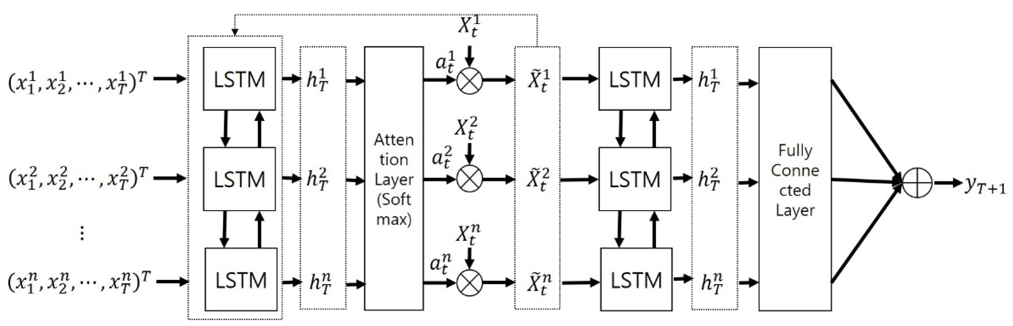
This section describes both the overall structure of the prediction system and also the roles of each component used for predicting the yields of tomatoes. The structure of the input attention-based LSTM model is given in Figure 1. The overall process of this network consists of two steps. First, by using n-data, each of which has a length of T, as an input, and putting it into the LSTM in Encoder, hidden states are created. Next, using the hidden states generated by the LSTM, attention contained in Encoder is applied to derive variables that have great significance among exogenous variables that influence the variable to be predicted.
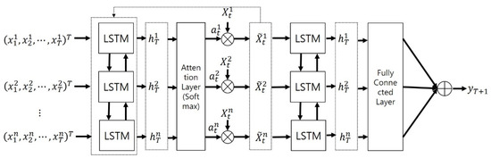
Figure 1.
Structure of input attention-based Encoder network.
The LSTM network, the first part of the attention-based Encoder network, is capable of learning long-term dependencies. It has the advantage of connecting previous information to the present task. Due to its special memory cell architecture, the LSTM network overcomes the defects of the traditional RNN, especially the problems of gradient disappearance and gradient explosion.
For time series prediction, given the input sequence with where is the number of exogeneous series, the encoder can be applied to learn a mapping from to with
where is the hidden state of the encode at time is the size of the hidden state, and is a non-linear activation function that could be an LSTM or gated recurrent unit (GRU). Here, we used an LSTM unit as to capture long-term dependencies. Each LSTM unit has a memory cell and three sigmoid gates: input gate , forget gate , and output gate . The update of an LSTM unit can be summarized as follows:
where is a concatenation of the previous hidden state and the current input denote the weight vector of the forget gate, input gate, output gate, memory cell, respectively, and are the bias vectors. Moreover, is a logistic sigmoid function and is an element wise multiplication. Equation (2) represents the forget gate and determines what information should be thrown away from the cell state, where denotes the output of the forget agate. Equations (3) and (4) represent the input gate, which decides what new information should be stored in the cell state, where and denote the output of the input gate, and denotes the activation vector of the current cell state. Equations (6) and (7) represent the output gate, where denotes the output of the output gate. and are the hidden state of the last cell and the current cell. Finally, the feature state matrix is the output of the LSTM layer.
The attention layer, the second part of the attention-based Encoder network, allows the model to capture the most important exogenous variables for yields of tomatoes when different features of past states are considered.
Given the -th input exogeneous series , we can construct an input attention mechanism via a multilayer perceptron, by referring to the previous hidden state and cell state in the encoder LSTM unit as
and
where , and are parameters to learn. Factor is the attention weight measuring the importance of the -th input exogenous series at time . The input attention mechanism is a feed forward network that can be jointly trained with other components of the LSTM. With these attention weights, we can adaptively extract the driving series with
Then the hidden state at time can be updated as:
where is an LSTM unit that can be computed according to Equations (2)–(7) with replaced by the newly computed . With the proposed input attention mechanism, the encoder can selectively focus on certain deriving series rather than treating all the input driving series equally.
Third, for non-linear autoregressive with exogenous (NARX) modeling, we aimed to use the multi-layer perceptron to approximate the function F so as to obtain an estimate of the current output with the observation of all inputs as well as previous outputs. Specifically, can be obtained with
where is the hidden state. The parameters and are the weights and biases of multilayer perceptron network.
2.2. Autoregressive Moving Average (ARMA)
The ARMA prediction model for time series is given as
where is a constant, is the number of autoregressive orders, is the number of moving average orders, is autoregressive coefficients, is moving average coefficients and is a normal white noise process with zero mean and variance .
As the ARMA models have numerous parameters and hyper-parameters, Box and Jenkins [1] suggest an iterative three-stage approach to estimate an ARIMA model. They are model identification, parameter estimation and model checking. First, model indemnification is the checking stationarity and seasonality, performing differencing if necessary, choosing model specification ARMA (p, q). To determine the orders of ARMA model, autocorrelation function (ACF) and partial autocorrelation function (PACF) are used in conjunction with the Akaike information criterion (AIC). Second, the parameter estimation is the computing coefficients that best fit the selected ARMA model using maximum likelihood estimation or non-linear least-squares estimation. Third, the model checking is the testing whether the obtained model conforms to the specifications of a stationary univariate process.
2.3. Hybrid Forecasting System using Attention-Based LSTM Network and ARMA Model
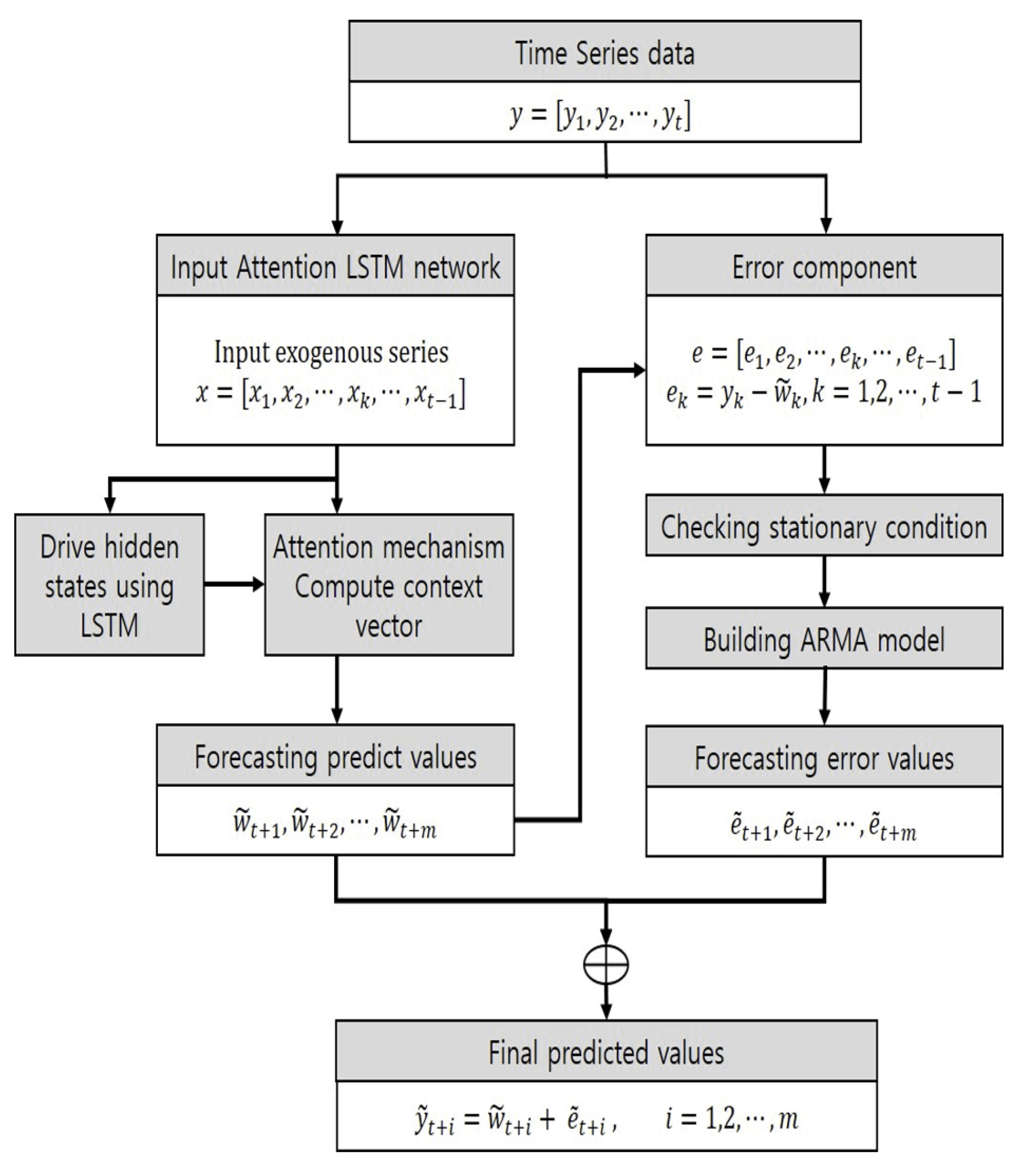
In general, it is difficult to accurately predict the yield due to the small amount of fruit or vegetable data collected at the cultivation site. Hence, none of ARMA and attention-based LSTM network is a suitable model for forecasting this kind of data. First, for a small amount of time series data, an attention-based LSTM network is applied to calculate a rough predicted value for the yield. Next, the difference between the predicted value generated through the LSTM network and the actual observed value can be corrected using an appropriate statistical model. Thus, we can combine the two models to form a system that can more accurately predict yields. The progress of a new prediction system that will implement this idea can be progressed through the following five steps.
- Step 1:
- We train an attention-based LMTM network using learning data including several exogenous factors and yields collected.
- Step 2:
- We use the validation data as input to the learned attention-based LSTM to generate predicted values for yields.,
- Step 3:
- We use the actual time series dataof the yields and the predicted time series datapredicted by the model to create the residual time series data as follows..
- Step 4:
- We construct an ARMA model for the generated error time series data and generate a predicted value of the error for the future point in time.
- Step 5:
- We add the predicted time series value () by the attention-based LSTM model in step 2 and the error value () predicted by the ARMA model in step 4 to get the time series predicted value at time t + 1 as follows..
The Figure 2 is shown as diagrammatically illustrating the progress of the new prediction system described so far.
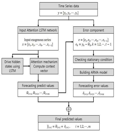
Figure 2.
Hybrid forecasting system Using attention-based LSTM network and ARMA model.
3. Experimental Results
This section describes the dataset for empirical studied and the graphical analysis conducted for all of variables for the time series dataset. Finally, we compared the proposed attention-based LSTM model against other existing methods and interpreted the input attention for exogenous variables as well as the efficiency of prediction for tomato yield.
3.1. Datasets
The dataset used in this study consisted of data from a total of 83 farm households collected from 2017 to 2018 and from 2018 to 2019 in three regions, including Gyeongam, Jeonbuk, and Jeonnam, in South Korea. As the value of the response variable, the yield of tomatoes observed at a total of 31 time lags every week was used. In addition, as exogenous variables, a total of 15 time series data such as the minimum, maximum and average values of the internal temperature, external temperature, internal humidity, and CO2 concentration observed during the same period were used. The collected data are summarized in Table 1. Jędrszczyk et al. [18] and Greco et al. [19] mentioned the rainfall item as one of the exogenous variables, but since this study does not consider a model that predicts the yield of tomatoes grown in the field, but rather considers exogenous variables that affect tomato yield in a facility, it is considered that there is no need to consider rainfall in particular, and it was excluded from consideration. Instead, this study found that humidity rather than rainfall affects yield in facility cultivation, so the experiment was conducted considering the maximum, minimum, and average humidity for day/night humidity.

Table 1.
Information of collected exogenous variables for tomatoes.
3.2. Association Analysis
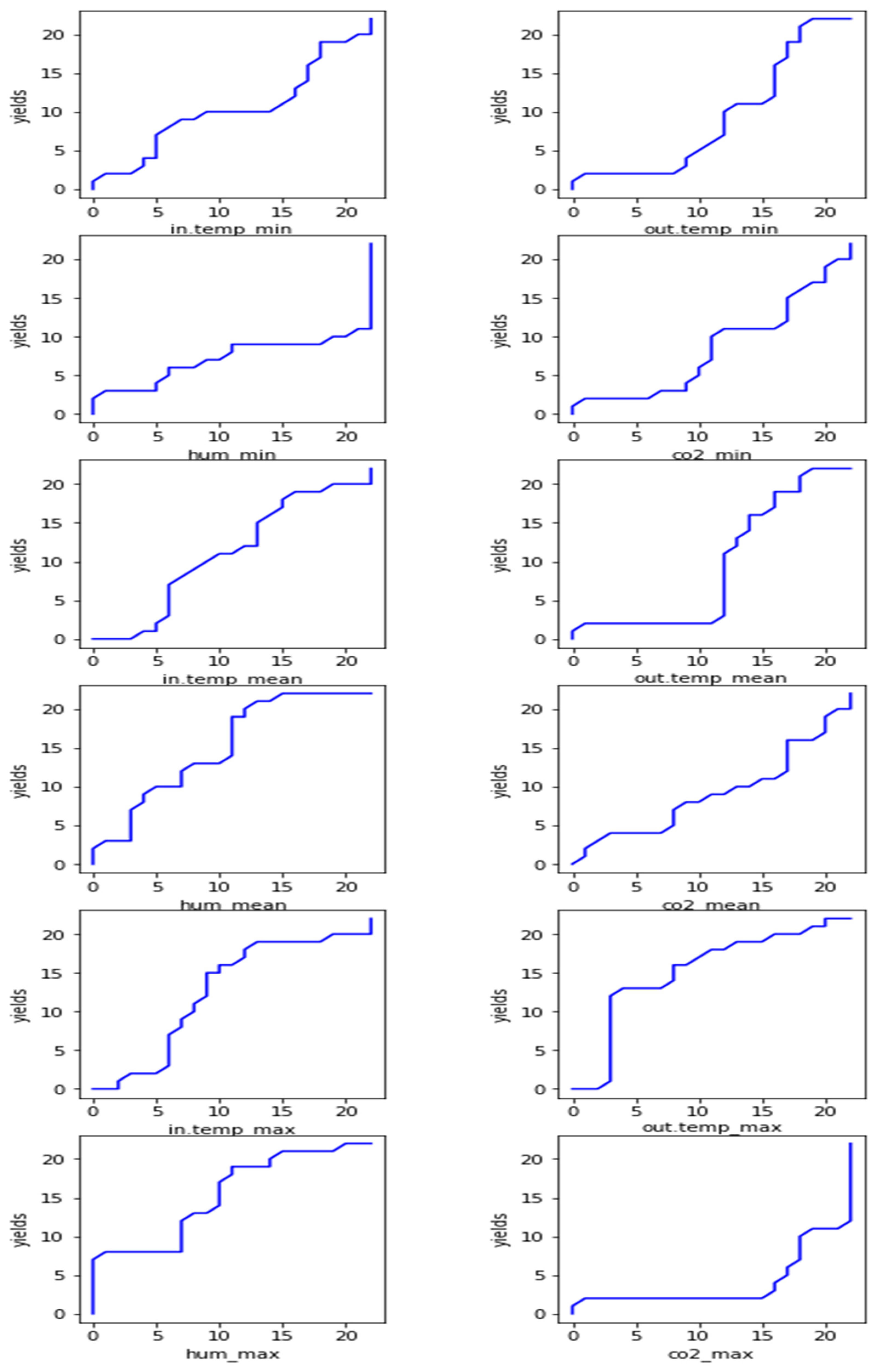
First, we used the DTW technique to analyze the correlation between tomato yields and environmental variables affecting the yields. Table 2 and Figure 3 show the DTW distance and DTW matching graphics between the tomato yields and 12 environmental factors.
Table 2.
DTW distance between environment variables and tomato yields.
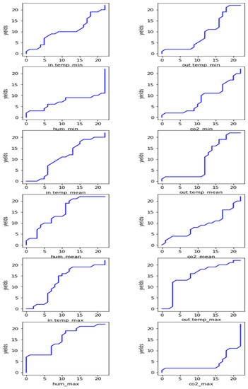
Figure 3.
Correlation between environment variables and tomato yields by DTW.
Here, the smaller the distance or the closer the shape of the graph is to a straight line, the more environmental factors affecting the tomato yields can be found. From the following two results, we found that the minimum and average values of the internal temperature, and the minimum and average values of CO2 have great influence on the yields of the tomatoes.
Next, we conducted a correlation analysis to numerically evaluate the relationship between the yields and each environmental variable. From the results shown in Table 3, we note that the minimum, average, and maximum values of the internal temperature and the minimum and average values of CO2 have a positive correlation with the tomato yield, but it turned out that the average and the maximum of the internal humidity has a negative correlation with the tomato yields.
Table 3.
Correlation coefficients between tomato yields and environmental factors.
Therefore, from the above two analysis results, we conclude that the internal temperature, CO2 and internal humidity are the environmental factors that have a great influence on the tomato yield. However, it was found that the internal temperature and CO2 had a positive correlation with the yields, but on the contrary, the internal humidity had a negative correlation with the yields. Therefore, to increase the yields when growing tomatoes, it is recommended to increase the internal temperature and the level of CO2, and on the contrary, it is desirable to reduce the internal humidity.
3.3. Prediction by Attention-Based LSTM
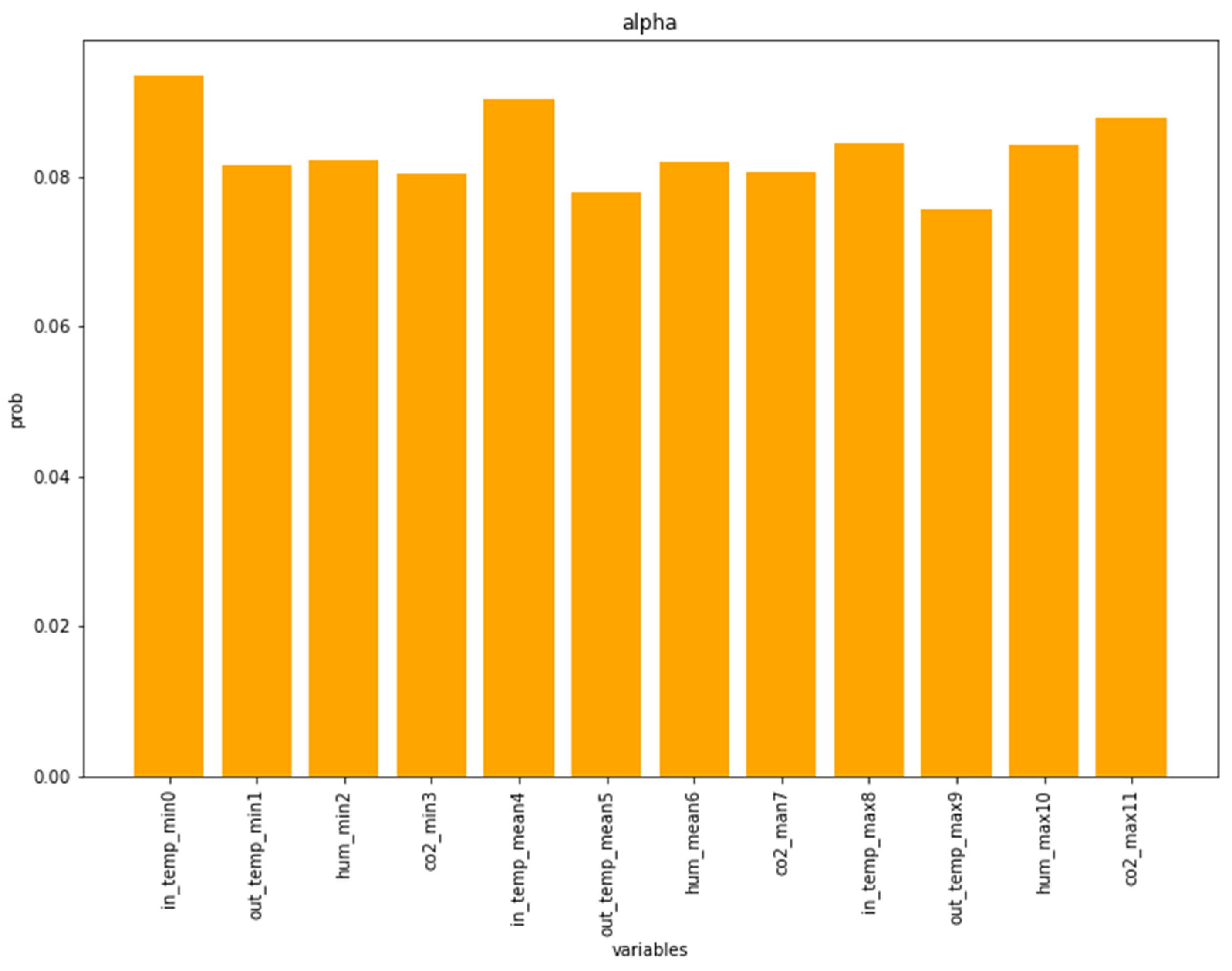
In prediction step, firstly, we trained the attention-based LSTM network using the 73-farmhouse data and calculated standardized attention weights to find out which environmental variables affect the tomato yield. In the LSTM model, we used MSE (mean square error) as the loss function and Adam’s optimizer as the optimization algorithm. The learning rate was 0.001, 32 input attention LSTM units were used, 32 encoder LSTM units were used, and 100 repetitions of train epochs were used. Figure 4 shows the histogram of the weights for each exogenous variable. Figure 4 shows that the environmental factors that greatly influence the tomato yields are the internal minimum temperature, inter temperature mean, internal temperature maximum, maximum humidity and the maximum CO2. The results given here are very similar to those given by the DTW discussed above.
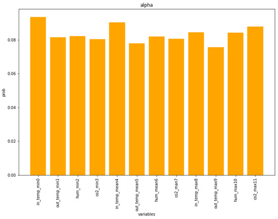
Figure 4.
Attention weights for input environmental variables.
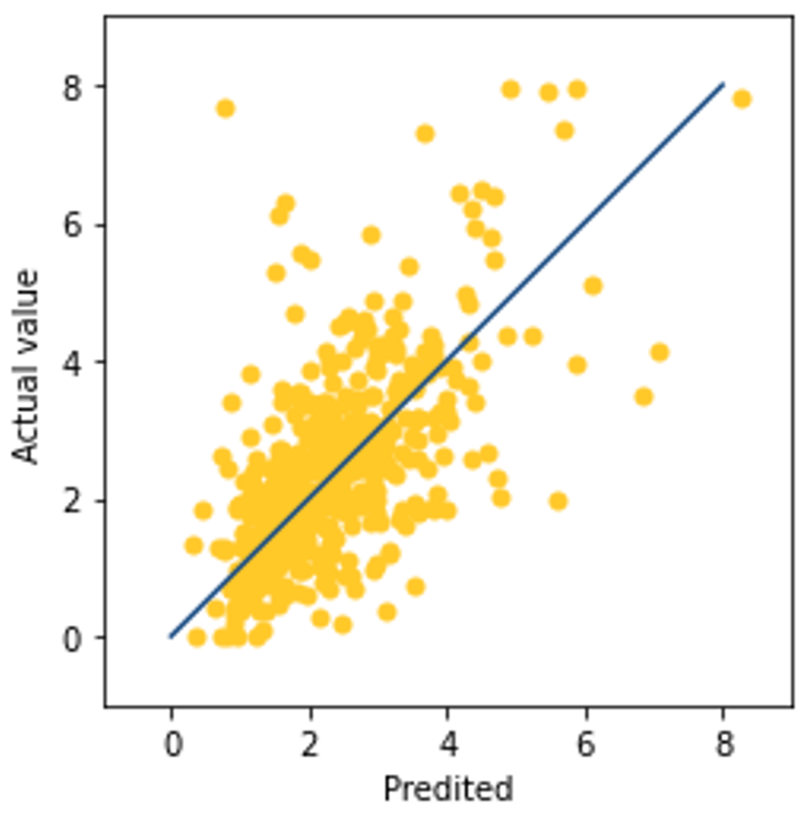
Secondly, we created a two-dimensional scatterplot for the observed values and predicted values generated by the trained attention-based LSTM using the 10-testing data. Figure 5 shows that the state-based LSTM model has a large difference between the measured and predicted values for the overall testing farms data.

Figure 5.
Scatterplot between predicted values and actual values.
3.4. Prediction by Hybrid Methods
We conducted an experiment to find out the performance of the proposed method. The data used in the experiment were the tomato production produced by a total of 83 farms each week, and the production of 73 farms among them was used as a dataset to train the input attention-based LSTM. The output of the remaining 10 farms was used to analyze the performance of the proposed method.
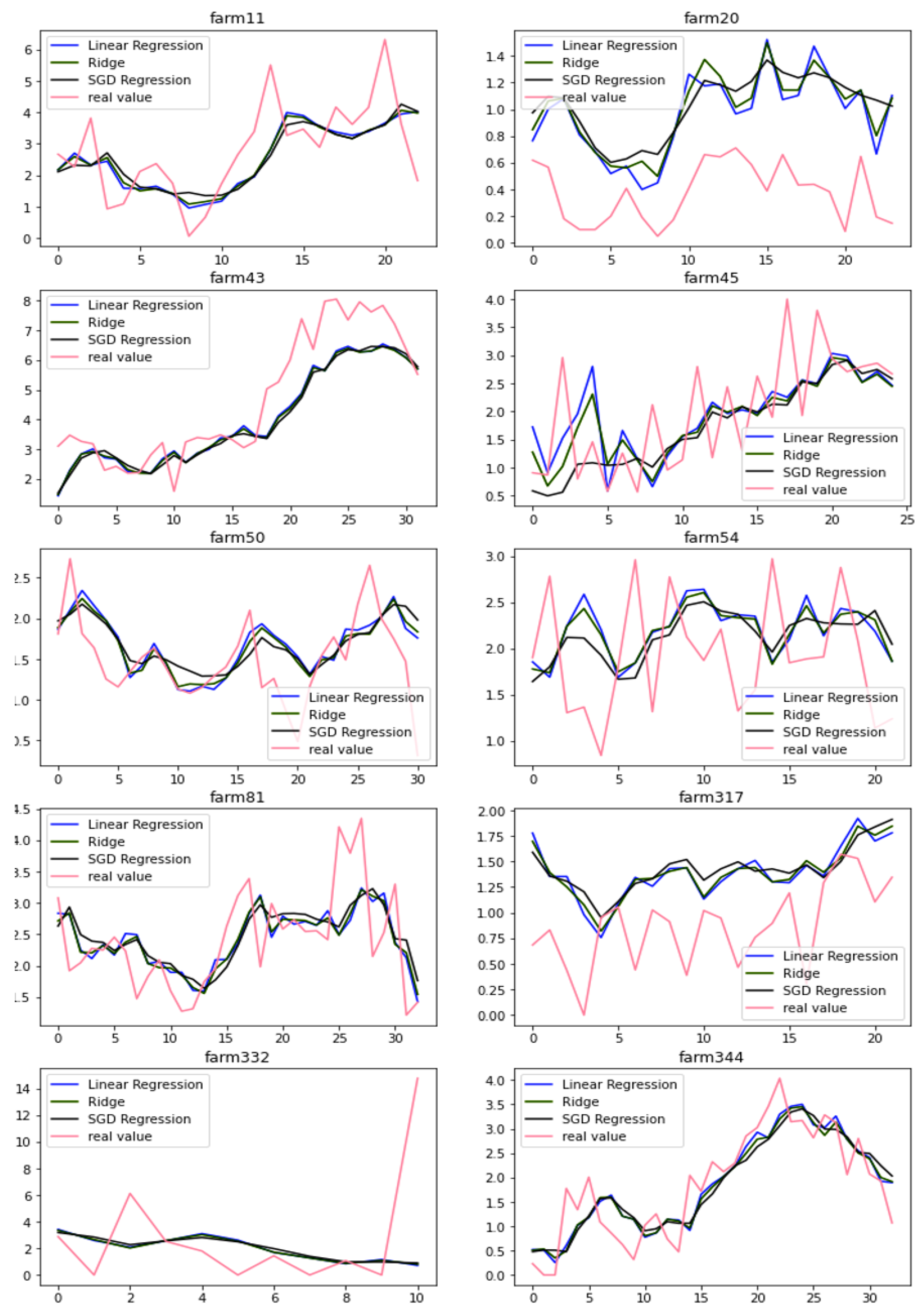
First, we configured the data in units of T = 5-time steps to learn the input attention-based LSTM and regression models. We used 70% of the total 2030 datasets for training and 30% for validation. Separately, 256 samples were used as test data. To select the optimal time T, we examined the effect of each environmental factor on the yield for each week. To this end, the model was trained using the actual yield and the values of environmental variables from T = 3 to T = 15 in units of one week based on the yield. As a result of calculating the RMSE using the validation data with the trained model, the RMSE value was the lowest when the time point was T = 5, so we selected T = 5. Next, the (p, q) order of the ARMA model for predicting the error component of the proposed method was set to (2, 0). To determine the optimal (p, q) in ARMA (p, q), we iteratively assumed the model for p from 0 to 3 and q from 0 to 3 and computed the autocorrelation function [15]. Therefore, the value that maximizes autocorrelation (p = 2, q = 0) was selected. Figure 6 shows the results of predicting tomato yield using traditional regression models such as linear, ridge, and SGD regression. At this time, the same 12 environmental factor values were used as input values for each time period, and the yield at that time was used as the response variable value. In Figure 6, the x-axis represents the lag in weeks, and the y-axis shows the predicted yield and the actual measured yield of the three models corresponding to the lag. Yields prediction by the traditional regression method shows comparatively similar predictive power. However, many prediction errors occur on harvest days where there is a sudden change in yields. Since the cultivation methods are different for each growing farm, environmental factors are also slightly different for each farm, and the measurement accuracy is also different for each farmer, so there was a deviation between the measured value and the predicted value. This result can be attributed to the limitations of the existing multiple linear regression model as well as the inaccuracy of the farmers’ measurements.
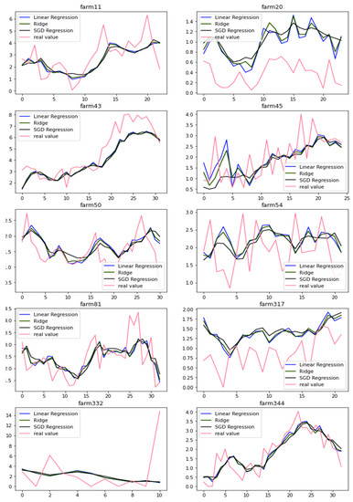
Figure 6.
Scatterplot between predicted values and actual values.
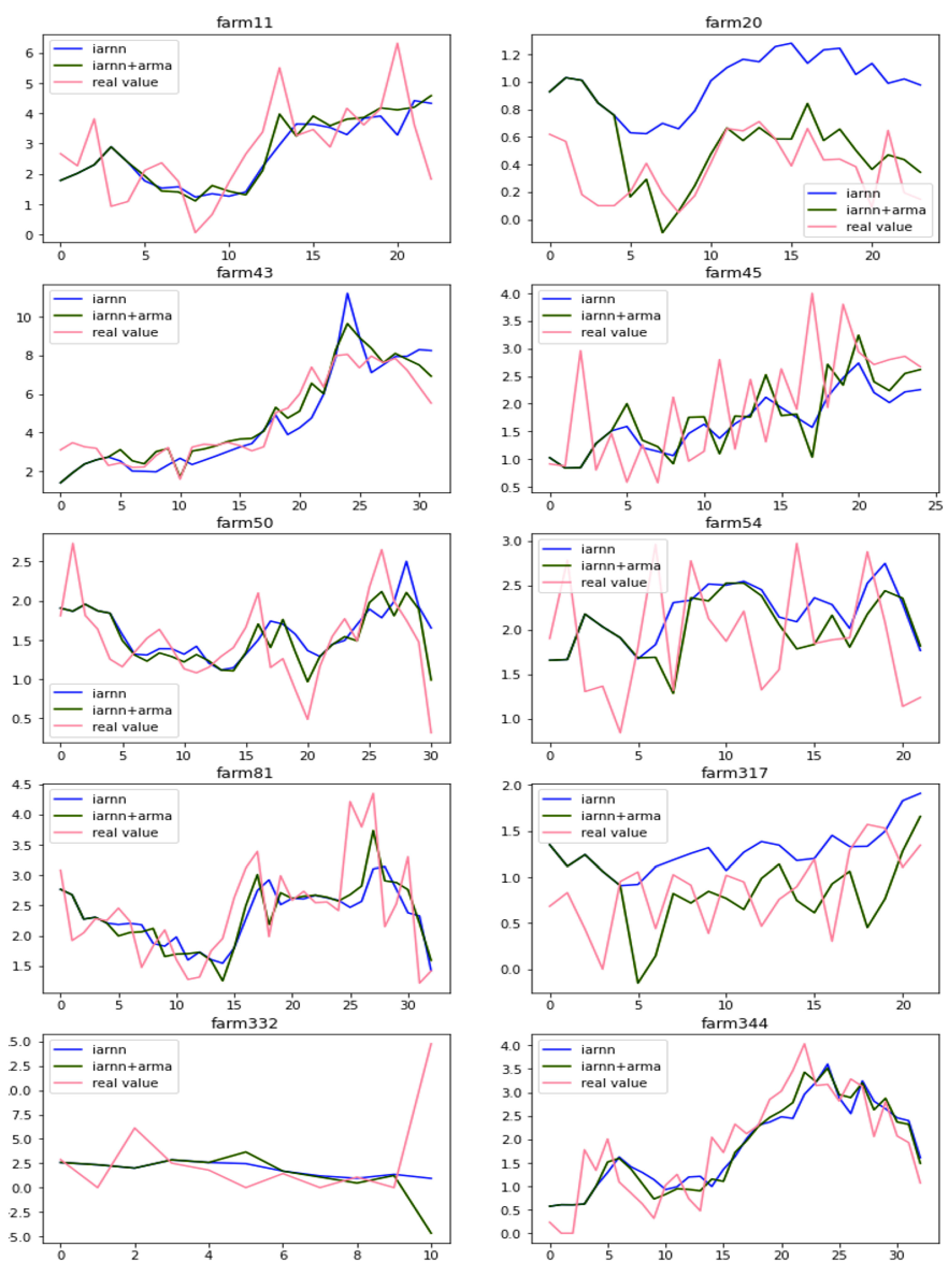
Figure 7 shows that the results of predicting tomato production for 10 randomly selected farms. In Figure 7, the blue solid line shows the result of predicting the production volume using the input attention-based RNN (IARNN), and the green solid line shows the output prediction result using the method combining the input attention-based LSTM and the ARMA model (IARNN + ARMA). The red line shows the actual production. As shown in Figure 7, if we analyze it graphically, the trend of almost all farms’ tomato production can be predicted well. In particular, farmers No. 54 and No. 317 showed good predictions even when there were large fluctuations in tomato production per week.
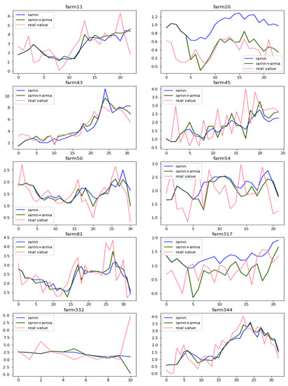
Figure 7.
Comparison results of tomato yields prediction using input attention-based RNN and the proposed method.
The following numerically compares the prediction performance of the proposed method with the input attention-based RNN (IARNN) using mean square error. It can be seen from numerical comparison that the proposed method shows better performance. However, as can be seen from the graphical and numerical analysis, the performance of farmhouse 332 is not good. This is because the proposed method uses the ARMA model to compensate for the error component, and a certain amount of time series data is required to estimate this error component in the ARMA model. However, it was difficult to accurately predict the error component because the production period of farm 332 was relatively too short (as shown in Table 4).
Table 4.
Mean square error for several time series data analysis methods.
4. Conclusions
In this paper, we tried to predict how various environmental factors with time series information affect the yields of tomatoes by combining a traditional statistical time series model and a deep learning model. In the first half of the proposed model, we use an encoding attention-based LSTM network to identify environmental variables that affect the time series data for tomatoes yields. In the second half of the proposed model, we used the ARMA model as a statistical time series analysis model to improve the difference between the actual yields and the predicted yields given by the attention-based LSTM network at the first half of the proposed model. Next, we predicted the yields of tomatoes in the future based on the measured values of environmental variables given during the observed period using a model built by integrating the two models. Finally, the proposed model was applied to determine which environmental factors affect tomato production, and at the same time, an experiment was conducted to investigate how well the yields of tomatoes could be predicted. From the results of the experiments, it was found that the proposed method predicts the response value using exogenous variables more efficiently and better than the existing models. In addition, we found that the environmental factors that greatly affect the yields of tomatoes are internal temperature, internal humidity, and CO2 level. In the future, the research direction is to apply the proposed hybrid model to predicting the yield of crops grown in various facilities such as strawberries, watermelons, melon, and cucumbers as well as tomatoes.
Author Contributions
Conceptualization, W.C., S.K., M.-H.N. and I.N.; methodology, W.C.; software, S.K.; validation, W.C. and I.N.; formal analysis, S.K.; investigation, W.C.; resources, M.-H.N.; data curation, W.C. and I.N.; writing—original draft preparation, W.C. and S.K.; writing—review and editing, I.N. and W.C.; visualization, S.K.; supervision, W.C. and I.N.; project administration, W.C. and M.-H.N.; funding acquisition, I.N. All authors have read and agreed to the published version of the manuscript.
Funding
This research was funded by research fund from Chosun University, 2019.
Conflicts of Interest
The authors declare no conflict of interest.
References
- Box, G.E.P.; Jenkins, G.M.; Reinsel, G.C.; Ljung, G.M. Time series analysis: Forecasting and Control, 5th ed.; Wiley: San Francisco, CA, USA, 2015. [Google Scholar]
- Nelson, B.K. Time Series Analysis Using Autoregressive Integrated Moving Average (ARIMA) Models. Acad. Emerg. Med. 1998, 5, 739–744. [Google Scholar] [CrossRef] [PubMed]
- Engle, R.F. Autoregressive Conditional Heteroskedasticity with Estimates of The Variance of United Kindom Inflation. Econometrika 1982, 50, 987–1007. [Google Scholar] [CrossRef]
- Pham, H.T.; Tran, V.T.; Yang, B.S. A Hybrid of Nonlinear Autoregressive Model with Exogenous Input and Autoregressive Moving Average Model for Long-Term Machine State Forecasting. Expert Syst. Appl. 2010, 37, 3310–3317. [Google Scholar] [CrossRef] [Green Version]
- Men, Z.; Yee, E.; Lien, F.S.; Yang, Z.; Liu, Y. Ensemble Nonlinear Autoregressive Exogenous Artificial Neural Networks for Short-Term Wind Speed and Power Forecasting. Int. Sch. Res. Not. 2014, 2014, 1–16. [Google Scholar] [CrossRef] [PubMed] [Green Version]
- Boussaada, Z.; Curea, O.; Remaci, A.; Camblong, H.; Bellaaj, N.M. A Nonlinear Autoregressive Exogenous (NARX) Neural Network Model for the Prediction of the Daily Direct Solar Radiation. Energies 2018, 11, 620. [Google Scholar] [CrossRef] [Green Version]
- Huo, F.; Poo, A.N. Nonlinear autoregressive network with exogenous imputs based contour error reduction in CNC machines. Int. J. Mach. Tools Manuf. 2013, 67, 45–52. [Google Scholar] [CrossRef]
- Tang, L. Application of Nonlinear Autoregressive with Exogenous Input (NARX) neural network in macroeconomic forecasting, national goal setting and global competitiveness assessment. arXiv 2020, arXiv:2005.08735v1. [Google Scholar] [CrossRef]
- Hussain, S.A.; Yuen, R.K.K.; Lee, E.W.M. Energy Modeling with Nonlinear-Autoregressive Exogenous Neural Network. In E3S Web of Conferences; EDP Sciences: Ulis, France, 2019. [Google Scholar]
- Wibowo, A.; Pujianto, H.; Saputro, D.R.S. Nonlinear Autoregressive Exogenous Model (NARX) in Stock Price Index’s Prediction. In Proceedings of the 2017 2nd International Conferences on Information Technology, Information Systems and Electrical Engineering (ICITISEE), Yogyakarta, Indonesia, 1–3 November 2017. [Google Scholar]
- Mohammadi, K.; Eslami, H.R.; Kahawita, R. Parameter estimation of an ARMA model for river flow forecasting using goal programming. J. Hydrol. 2006, 331, 293–299. [Google Scholar] [CrossRef]
- Qin, Y.; Song, D.; Chen, H.; Jiang, G.; Cottrell, G.W. A Dual-Stage Attention-Based Recurrent Neural Network for Time Series Prediction. arXiv 2007, arXiv:1704-02971. [Google Scholar]
- Guo, T.; Lin, T.; Lu, Y. An Interpretable LSTM Neural Network for Autoregressive Exogenous Model. In Proceedings of the Workshop track of ICLR 2018, Vancouver, Canada, 30 April–3 May 2018; pp. 1–7. [Google Scholar]
- Lee, H. Bidirectional Encoder-Decoder with Dual-Stage Attention for Multivariate Time-Series Prediction. Master’s Thesis, Seoul National University, Seoul, Korea, 2019. (In Korean). [Google Scholar]
- Na, I.S.; Tran, C.; Nguyen, D.; Dinh, S. Facial UV map completion for pose-invariant face recognition: A novel adversarial approach based on coupled attention residual UNets. Hum. Cent. Comput. Inf. Sci. 2020, 10, 1–17. [Google Scholar] [CrossRef]
- Dang, T.X.; Oh, A.R.; Na, I.S.; Kim, S.H. The Role of Attention Mechanism and Multi-Feature in Image Captioning. ICMLSC 2019, 2019, 170–174. [Google Scholar]
- Ran, X.; Shan, Z.; Fang, Y.; Lin, C. An LSTM-Based Method with Attention Mechanism for Travel Time Prediction. Sensors 2019, 19, 861. [Google Scholar] [CrossRef] [PubMed] [Green Version]
- Jędrszczyk, E.; Skowera, B.; Gawęda, M.; Libik, M. The effect of temperature and precipitation conditions on the growth and development dynamics of five cultivars of processing tomato. Hortic. Sci. 2016, 24, 63–72. [Google Scholar] [CrossRef] [Green Version]
- Greco, A.; De Luca, D.L.; Avolio, E. Heavy Precipitation Systems in Calabria Region (Southern Italy): High-Resolution Observed Rainfall and Large-Scale Atmospheric Pattern Analysis. Water 2020, 12, 1468. [Google Scholar] [CrossRef]
Publisher’s Note: MDPI stays neutral with regard to jurisdictional claims in published maps and institutional affiliations. |
© 2021 by the authors. Licensee MDPI, Basel, Switzerland. This article is an open access article distributed under the terms and conditions of the Creative Commons Attribution (CC BY) license (https://creativecommons.org/licenses/by/4.0/).