Analytical Winding Power Loss Calculation in Gapped Magnetic Components

Abstract

The analytical calculation of winding loss in gapped magnetic components is complex, and numerical analysis tools, such as finite elements analysis (FEA) tools, are commonly needed to characterize the windings. As FEA tools are used, the required design time of these types of components increases greatly when many simulations are needed to select the appropriate component for a given application, and simple analytical models become necessary to reduce the design time. In this paper, some analytical approaches for winding loss calculation in gapped magnetic components are reviewed and a general two-dimensional equivalent method, which aims to consider the frequency effects in conductors in a simplified manner, is proposed afterward. Due to its simplicity, it can be integrated into design and optimization tools in order to evaluate the influence of the air gap over the winding loss even at the early stages of the design process. The presented model shows good agreement with FEA simulations and measurements.

1. Introduction

Accurate winding loss calculation in magnetic components used in power electronics applications is a very important task. Inaccurate calculations of the windings’ equivalent resistance can lead to under- or over-estimating the losses in the component, resulting in, for example, an unexpected temperature rise or a costly component oversize.

Many of the frequently used methods for the winding loss calculations assume the one-dimensional field in order to evaluate the eddy currents’ effects in the conductors [1,2,3,4,5]. The most frequent approach, often called the Dowell method [1], consists of dividing the windings into portions, considering every portion as an equivalent foil conductor with an equal total sectional area and multiplying the DC resistance of each layer by a corresponding factor to obtain the AC resistance of the winding. This method, although simple, has considerable errors at high frequencies [2,3,4,5,6,7]. Since Dowell and Dowell-based methods assume a one-directional magnetic field over the windings of the component, they do not properly model the winding loss in components where this assumption cannot be made, which is the case of components with air gaps where the windings; besides, the skin and proximity (to neighbor conductors) effects that are already considered in 1D methods, will be influenced by the fringing field of the gap, and such an influence will be reflected as an increment of the equivalent resistance [6,7,8,9]. In this situation, even if the windings could be easily converted into equivalent layers, the magnetic field along the window breath is far from being considered as one-dimensional, and therefore, classical Dowell and many 1D approaches cannot be properly applied and might lead to considerable errors in the estimation of the equivalent resistance. This can be seen Figure 1, where the calculated equivalent resistance in a one-layer gapped inductor by means of both the Dowell equation and FEA results is compared.

In the case of gapped magnetic components, 2D effects are particularly important in the estimation of the winding loss because they can be the major contributors in the loss mechanism [8]. Since the analytical evaluation of the gap influence in the winding loss is still very limited, FEA tools are commonly needed in order to characterize the windings of the component [10,11,12,13,14]. These numerical tools are considered very accurate, but, depending on the considered component or the number of required simulations, the analysis might be very expensive in terms of time. This is particularly disadvantageous in a design process where many cases should be considered in order to optimize, for example, an inductor for a given application in terms of winding loss. Therefore, accurate models for the analytical calculation of winding loss in gapped magnetic components are needed.

In this paper, some available 2D analytical approaches for power loss calculation in the windings of magnetic components are reviewed in Section 2. Afterwards, a method based on a simplified magnetic field calculation is presented and compared with FEA results and measurements. The proposed method, which is explained in Section 3, is suitable for calculations in the low–medium-frequency range in situations where the conductors might be selected to stand a given DC current rather than avoiding or reducing the frequency effects (in other words, in conductors with a bigger size than the proper one according to the operating frequency; this may be the case of a power inductor that operates with a considerable current ripple and a very large DC current). Validation, results, and application examples, as well as comparisons with the measurements are given in Section 4 and Section 5, respectively, followed by the conclusions in Section 6.

2. Review of 2D Analytical Approaches

Many methods used for the calculation of conduction loss in magnetic components are based on the widely accepted winding loss separation concept, which allows the independent calculation of the considered loss mechanisms. Then, under this concept, the total winding loss is found to be the superposition of all loss components (DC, skin, proximity). This concept allows the calculation of conduction loss by “modules” offering the possibility to evaluate each component of the loss in a different way, giving us flexibility in choosing a desired approach to estimate the different contributions in the winding loss mechanism.

Despite the advantages, the loss separation concept is not always applicable. If it is applied out of its application scope, the power loss can be very different than the calculated value [15]. A general typical condition where loss separation can be used, among others and according to [15], is when the functions of the current densities are orthogonal in space. Nevertheless, the utilization of this concept is very interesting, and it can be used independently of the assumed geometry of the fields (in both 1D and 2D winding structures).

In 1D approaches, the loss separation method is applied by means of the calculation of the skin and proximity effects separately thanks to their orthogonality [2,3,4,5,6,16]. In 2D field distributions, such as gapped components, the concept of loss separation is also used. In such cases, the fringing field of the air gap is considered and introduced into the calculations as a part of the external magnetic field, which is used to estimate the power loss in the conductor due to the influence of such fields, which means that, in this kind of structures, the field calculation is an important “intermediate” step to estimate the winding loss (specifically, to calculate the proximity loss component).

Some simple approaches try to consider the effects of 2D proximity fields in 1D winding structures by means of a correction factor fitted from 2D FEA results [5,6,7] (avoiding in this way the step of calculating the fields). Although the approach is very simple and the reported results are in accordance with the experimental data, they can be applied only in components whose windings are arranged in a specific “layered” structure since they keep some of the limitations of 1D models and are not valid for components with incomplete layers. On the other hand, many methods [17,18,19,20,21,22,23,24,25,26,27,28,29,30,31,32] use the “intermediate step” of calculating the external magnetic field in order to evaluate the proximity loss, but the focus and application of each one, as well as the way that fields and the total winding loss are calculated are rather different. In this context, in order to facilitate the transition to the proposed method and having in mind that this paper is focused on the calculation of proximity loss (using a two-step calculation process: calculating fields and evaluating proximity loss using the previously calculated fields), this review is structured around two topics: the methods of calculating the overall magnetic field and the methods for the calculation of the loss in a conductor given an external magnetic field.

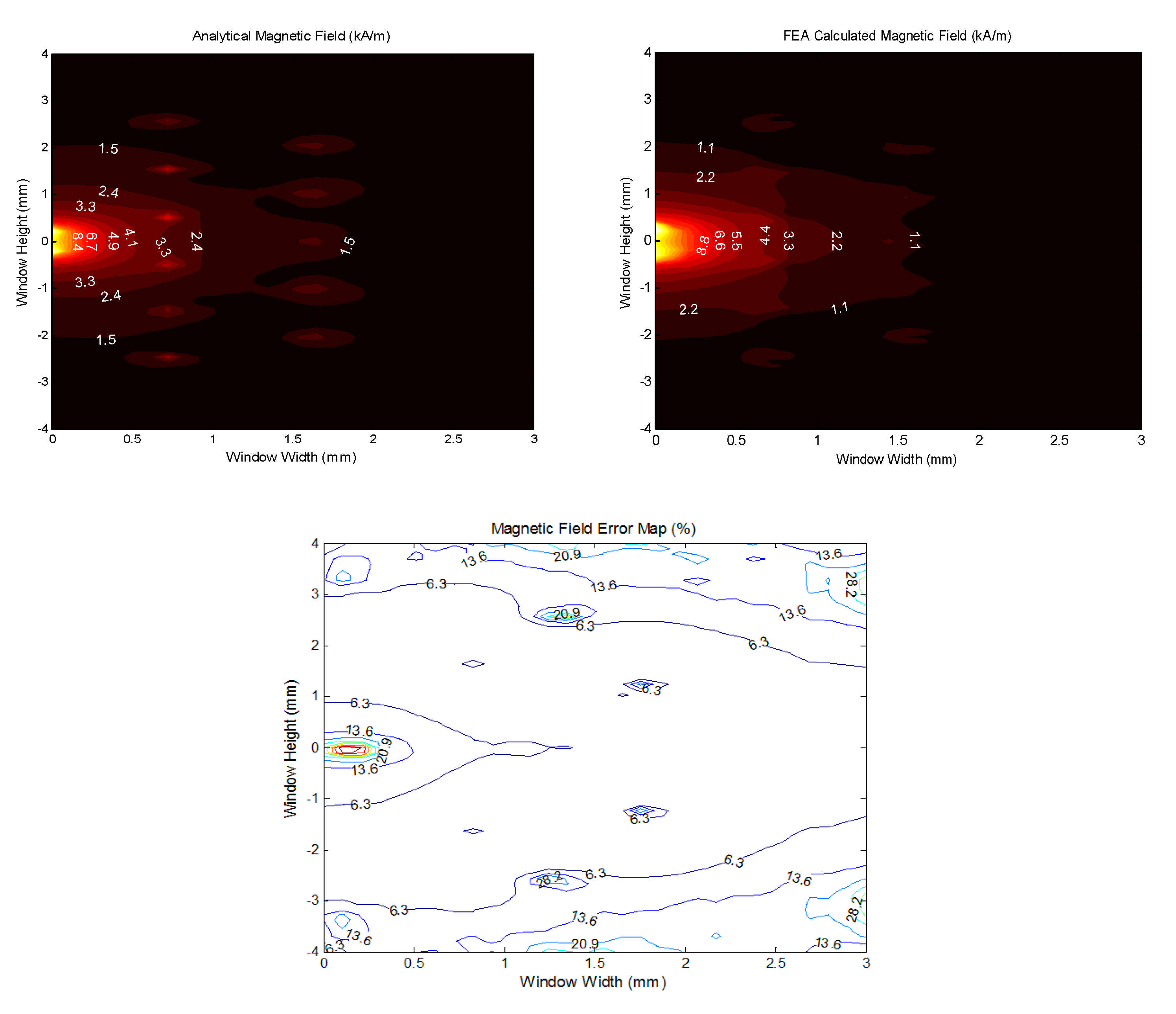
2.1. Methods for Calculating the Overall Magnetic Field

In terms of the magnetic field calculation, the different alternatives used for the determination of the field distribution in [17,18,19,20,21,22,23,24,25,26,27,28,29,30,31,32] can be classified into two general categories: numerical and analytical methods. Several approaches use the numerical calculation of the fields [23,24,25,26,27], resulting in a combined method to calculate the winding loss (numerical/analytical). This approach is a very good option in terms of accuracy since numerical tools, such as FEA, are used for the intermediate step of calculating the fields, reducing, as a consequence, the errors in the estimations.

When it comes to analytical calculations, the external magnetic field H can be evaluated by means of the magnetic potential (in the form of either the vector or scalar potential) that fulfils the Laplace equation. This approach was used in [17,21,22,29,31], but it results in complex equations that might be very difficult to implement (if its integration in a design and optimization tool is the objective). Another interesting approach, due to its simplicity, but perhaps being less accurate, is the calculation of the fields by means of the Biot–Savart law, applying the mirror-image technique [18,19,20], where the fringing field due to the air gap (which represents the core influence for the external magnetic field) can be considered by replacing the air gap with an equivalent current sheet that “emits” the same magnetic field as the air gap. This approach allows a tradeoff between accuracy and computational effort by choosing an appropriate number of images. In [15], different methods for calculating the magnetic fields were also reviewed and discussed.

2.2. Conduction Loss Calculations in the Presence of a Given Magnetic Field

Once the magnetic field has been calculated, the conduction loss in the wires can be estimated. For that purpose, most approaches use either the low-frequency approximation or a combination of magnetostatic field calculations and analysis with Bessel functions for the calculation of the power loss (both because of the evaluation of Poynting’s law). The low-frequency approximation, used in [17,18,19,23,25,32] and also discussed in [15,30], considers that the wire is small compared to the skin depth. This is a valid assumption in the case of litz wire or when the size of the wires has been selected according to the operating frequency (which is a common design criteria), but not adequate in cases where the diameter of the conductor is larger than twice the skin depth.

The Bessel function approach is used to “capture” the frequency dependence of the loss in the wire and can be used in those situations where the wire is no longer small compared with the skin depth at the considered frequency. It was used in [4,15,22,26,27,28]. Although it is exact for a single conductor in free space, it has been pointed out that this approach is not accurate in closely packed wires at high frequencies [2,3,33], and alternatives to improve the accuracy of the calculations have been proposed (basically based on numerical calculations).

Another interesting (and worth mentioning) method of calculating the winding loss is the complex permeability approach. Since it is a rather different approach to the methods discussed here, and for this reason is out of the scope of the paper, we refer the readers to [15,33,34,35,36,37,38] for more information.

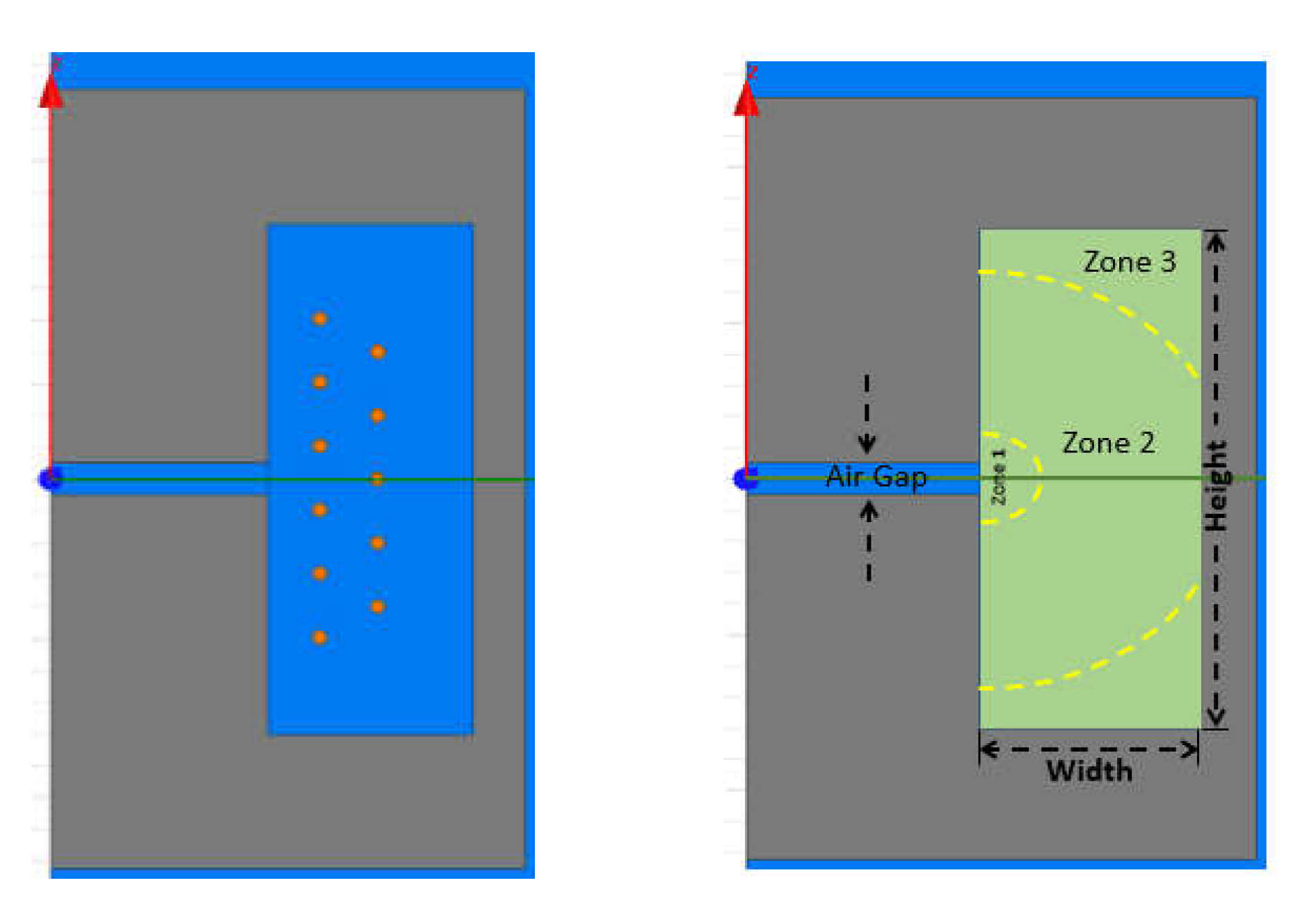
3. Proposed 2D Analytical Model

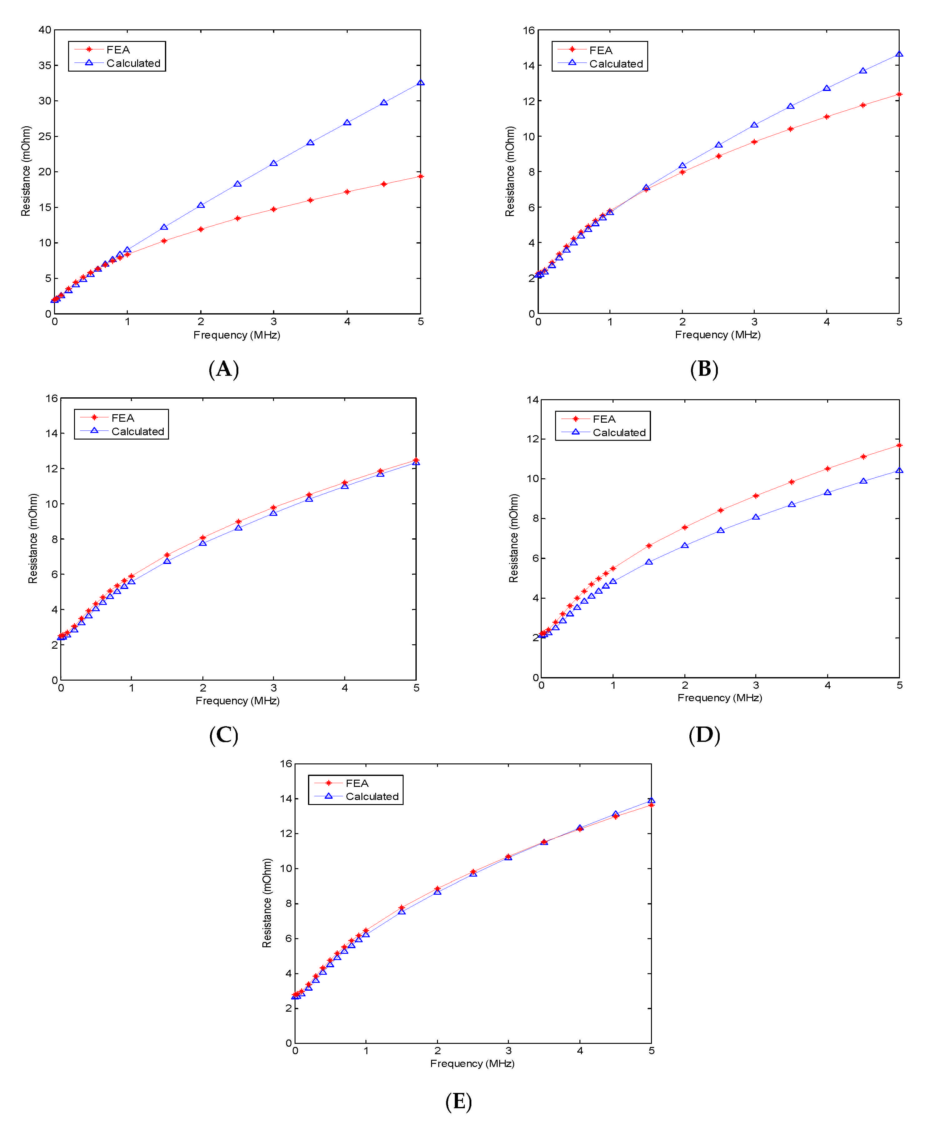
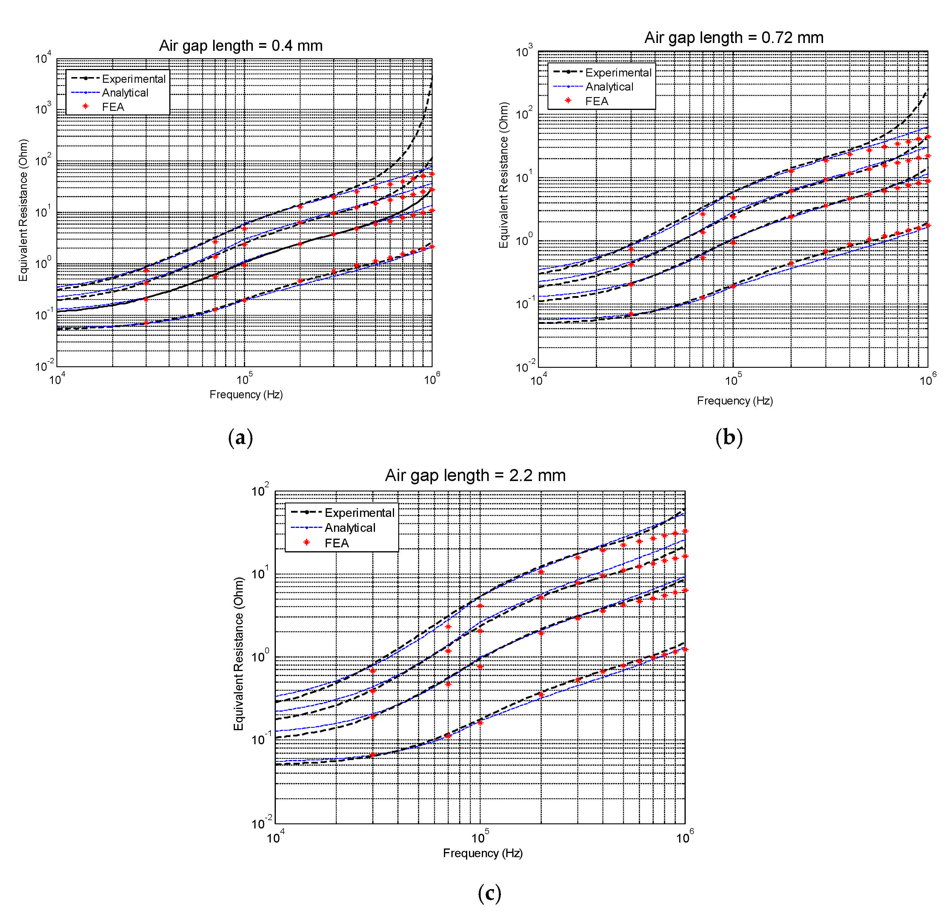
The proposed analytical model consists of the combination of a simple calculation of the fields and the Bessel function approach for the frequency-dependent loss evaluation. This combination allows the use of the proposed method in situations where the conductor’s size has not been selected according to the operating frequency (which might be the case of an inductor that operates with high average values of the currents and high ripples) and facilitates, due to its simplicity in the calculation of the fields, its implementation in CAD tools. The derivation of the proposed model is detailed below.

Expression (1) [30] corresponds to the power losses per unit length of a cylindrical conductor under a homogeneous transverse magnetic field, where ber, bei, ber’, bei’, ber₂, and bei₂ are, respectively, the real and imaginary part of the Bessel functions of first kind (of first or second order) and their derivatives, σ, µ, and µ₀ the conductivity, the relative permeability of the conductive material, and the permeability of free space, r the radius of the conductor, H₀ the magnitude of the external transverse field to the conductor, $k=\sqrt{w\sigma \mu {\mu }_0}$, and w the angular frequency.

$$P\left(W/m\right)=\frac{4\pi {\left(\mu {\mu }_0\right)}^2}{\sigma }kr{H}_0^2\frac{ber\left(kr\right)be{i}^{\text{'}}\left(kr\right)-be{r}^{\text{'}}\left(kr\right)bei\left(kr\right)}{{\left[{\mu }_0\left(\mu +1\right)ber\left(kr\right)+{\mu }_0\left(\mu -1\right)be{r}_2\left(kr\right)\right]}^2+{\left[{\mu }_0\left(\mu +1\right)bei\left(kr\right)+{\mu }_0\left(\mu -1\right)be{i}_2\left(kr\right)\right]}^2}$$

(1)

If the value of the relative permeability of the conductive material is approximately unity, which is the case of copper, (1) can be simplified as (2) without any significant difference.

$$P\left(W/m\right)=\frac{\pi {\left(\mu {\mu }_0\right)}^2}{\sigma }kr{H}_0^2\frac{ber\left(kr\right)be{i}^{\text{'}}\left(kr\right)-be{r}^{\text{'}}\left(kr\right)bei\left(kr\right)}{{\left[\mu {\mu }_{0}ber\left(kr\right)\right]}^2+{\left[\mu {\mu }_{0}bei\left(kr\right)\right]}^2}$$

(2)

Let us consider the fringing field due to an air gap in a magnetic component, H_a, two-directional in the plain xy in Cartesian coordinates, Expression (3). Any conductor affected by this fringing field will be exposed to its two components, H_x and H_y, both transversal to the conductor ($\widehat{x}$ and $\widehat{y}$ are unitary vectors in their respective directions; the conductor is longitudinal to the z axis). The evaluation of each component of (3) in (2) yields Equation (4), and the dissipated power per unit length in the conductor, P_a, can be expressed as the sum of both components of the dissipated power (5).

$${\stackrel{\rightharpoonup }{H}}_a=H_x\widehat{x}+H_y\widehat{y}$$

(3)

$$P_{x,y}=\frac{\pi {\left(\mu {\mu }_0\right)}^2}{\sigma }kr{\left(H_{x,y}\right)}^2\frac{ber\left(kr\right)be{i}^{\text{'}}\left(kr\right)-be{r}^{\text{'}}\left(kr\right)bei\left(kr\right)}{{\left[\mu {\mu }_{0}ber\left(kr\right)\right]}^2+{\left[\mu {\mu }_{0}bei\left(kr\right)\right]}^2}$$

(4)

$$P_a=P_x+P_y$$

(5)

The field components of H_a can be calculated, according to [17], with (6) and (7) for the x and y components, respectively, where l_g is half of the air gap length, x and y are the Cartesian coordinates with respect to the origin (see Figure 2), m is equal to zero if $x^2+y^2>l_g^2$ and 1 if $x^2+y^2<l_g^2$, and $H_g\cong 0.9NI/2l_g$ with N and I being the number of turns and the current through the winding, respectively. These equations, however, are limited to components whose air gap is placed in a symmetrical position with respect to the core height. (Note that a rough estimation of the field Hg is used. According to the results presented in [17], this expression is accurate enough for the calculation of the reference Hg. However, in order to reduce the errors in the results, the expression $H_g\cong 0.9NI/2l_g$ can be replaced by a different and more accurate one.)

$$H_x\left(x,y\right)=\frac{H_g}{2\pi }\ln \left[\frac{x^2+{\left(y-l_g\right)}^2}{x^2+{\left(y+l_g\right)}^2}\right]$$

(6)

$$H_y\left(x,y\right)=-\frac{H_g}{\pi }\left[{\tan }^{-1}\left(\frac{2x{l}_g}{x^2+y^2-l_g^2}\right)+m\pi \right]$$

(7)

Only the fringing field is considered and the contribution of near conductors (proximity), and the effect of the current flowing through the conductor (skin effect) in the winding loss must be included in order to calculate the total power loss in the conductors of the magnetic component.

Since skin and proximity effects are orthogonal [4], we can evaluate the contribution in the winding loss of each effect independently. From [30], the equivalent resistance per unit length of a round conductor carrying an alternating current (skin effect) can be obtained by means of Expression (8). Then, the effect of the overall external field, which includes fringing and proximity fields, can be calculated using Expression (2).

$$R_s\left(\raisebox{1ex}{$\Omega $}\!\left/ \!\raisebox{-1ex}{$m$}\right.\right)=Re\left[\frac{j^{\frac{3}{2}}k}{2\pi r\sigma }\frac{Bessel{J}_0\left(j^{\frac{3}{2}}kr\right)}{Bessel{J}_1\left(j^{\frac{3}{2}}kr\right)}\right]$$

(8)

In order to simplify, a magnetostatic field situation was assumed, and fringing and proximity fields were considered as independent (and the superposition theorem can be used) with an ideal concentric pattern, as shown in Figure 2. Under this assumption, the Biot–Savart law (9) can be used to calculate the magnetic field that affects a single straight conductor of length L due to the electric current I flowing through a near conductor at a distance h by means of Expression (10), where $\widehat{h}$ is a unitary vector in the direction of h (in this case, since h is in the vertical axis direction and the direction of the current is in the z axis, the vector product $Id\stackrel{\rightharpoonup }{l}\times \widehat{h}$ is in the direction of x).

$$\mathrm{d}\stackrel{\rightharpoonup }{H_p}=\frac{1}{4\pi }\frac{Id\stackrel{\rightharpoonup }{l}\times \widehat{h}}{h^2}$$

(9)

$$\stackrel{\rightharpoonup }{H_p}=-\frac{I}{2\pi h}\frac{L}{\sqrt{L^2+h^2}}\left(\widehat{x}\right)$$

(10)

At this point, P_x and P_y are calculated assuming the external field, H₀, as the sum of the corresponding components of the fringing and proximity fields, Expression (11), and the total loss per unit length of the considered conductor is obtained as the sum of (8) multiplied by the square of the RMS current through the winding and (12), whose components are evaluated by means of (2) with corrected values of the magnetic field ($H_0^{\text{'}}$).

$$\stackrel{\rightharpoonup }{H_a}+\stackrel{\rightharpoonup }{H_p}=\stackrel{\rightharpoonup }{H_0^{\text{'}}}$$

(11)

$$P_p=P_x^{\text{'}}+P_y^{\text{'}}$$

(12)

4. Model Validation

Finite element analysis (FEA) was used to assess the accuracy of the proposed approach. The commercial finite element tool MAXWELL from ANSYS was used for all FEA calculations. First, the effect of the external fields (due to neighbor conductors and air gap separately) was evaluated. After that, the model was used to calculate the equivalent resistance of several cases, and the results were compared with FEA. Furthermore, as the field calculation is critical in the global accuracy of the results, the calculated field map was later compared with FEA results.

To evaluate the effect of proximity fields, let us consider two round copper neighbor conductors of 0.3 mm in radius and 1 m in length carrying a sinusoidal current of 1 Apeak (for component characterization, the equivalent resistance is considered to be independent of the conducted current as it depends on the properties of the materials, the frequency, and the “spatial distribution” of the winding with respect of the existing field. For this reason, in order to simplify the FEA setup and the post-processing of the results, a peak current of 1 A was used in all cases and, later, the same current was used for the analytical calculation but any current could be used for loss estimation.), separated by a distance x, as shown in Figure 3a. The magnetic field at the center of each conductor was calculated by means of (10), and the equivalent resistance of Conductor 1 was extracted from the calculated power loss evaluated by means of (12), with H_g = 0, and (8) as the distance between both conductors increases. The FEA setup for the analysis of the proximity effect between the considered adjacent conductors, as well as the results, in terms of normalized resistance, are shown in Figure 3b and Figure 4, respectively (a copper conductivity of 58 × 10⁶ S/m was used in FEA simulations).

Figure 5 shows an axisymmetric representation of an AWG24 round wire over a ferrite gapped magnetic core with a relative permeability of 1000 (For simplicity, 2D axis-symmetric analysis was used for the FEA simulations. The components were modeled in the FEA tool using the structure transformation described in [14]). The component in the figure was used for the comparison between FEA and the evaluation of the fringing field contribution in the winding loss by means of Equation (12), with H_p = 0, where the conductor is affected only by the fringing field due to the air gap in the magnetic core and the equivalent resistance due to the effect of the current flowing through the considered conductor. The conductor was placed in different positions with respect to the air gap (of different lengths), and the dissipated power was calculated.

The equivalent resistance was later obtained dividing the calculated power loss, by the square of the RMS value of the current (1 A peak) plus the skin effect resistance calculated by means of Equation (8), and compared with the FEA results in

Table 1. Comparison between the analytical and FEA-calculated equivalent resistance of a conductor of position (x, y) from the air gap at a frequency of 500 kHz.

Case	Conductor Position (mm)	Gap Length (mm)	Calculated Equivalent Resistance (mΩ)		Relative Error at 500 kHz (%)
			Analytical	FEA
A	(0.40, 0)	0.40	5.50	5.75	−4.35
B	(0.80, −0.60)	0.20	3.94	4.19	−5.97
C	(1.30, 1.50)	0.15	4.02	4.31	−6.73
D	(0.80, −2.50)	0.70	3.52	4.00	−12.00
E	(1.80, 0.50)	0.50	4.49	4.74	−5.27

. The characteristics of each case are summarized in Table 1.

Results in Figure 6 show that the error respect of FEA calculation varies as the conductor is placed in different positions with respect to the air gap. Since the Bessel function approach is accurate for single “non-packed” conductors, these errors are due to inaccuracies in the calculation of the magnetic field. In order to verify this, let us consider an inductor with 11 turns placed in a spaced distribution in the window breath (Figure 7) and compare the calculated field with FEM magnetostatic analysis in the form of a magnetic field contour plot in the window breath (Figure 8). If we divide the window in three zones (Figure 7), where Zones 1, 2, and 3 correspond to the area close to the air gap, the central region of the window, and the corners, respectively, it can be seen that the field estimation is more precise in Zone 2. (As far as the magnetic core is concerned, the proposed method only considers the fringing flux as a source of the magnetic field. This is, to a certain extent, to simplify the problem and allow the utilization of a very simple model to estimate the magnetic field due to the air gap. Thanks to this assumption, the accuracy is reduced in zones where the effect of the geometry of the core affects or modifies the assumed distribution. These zones include all the corners and edges that form the window area in the magnetic core, and the loss of accuracy can be compensated using different models to estimate the magnetic field.) In the closest region to the air gap and the corners, Zones 1 and 3, respectively, the error in the field estimation might be significant as the considered position becomes closer to those regions. This is the case of Figure 6a, where the conductor was placed pretty close to the air gap where the error of the calculated field with respect to the FEA result was about the maximum value (the magnitude of the error might depend on the geometrical distribution of the component. However, the zones that are shown in the figure were considered to be valid for any applicable case.) Nevertheless, in a “standard configuration” of inductors with concentric core geometries (such as EE, RM, ETD, POT, etc.), the corresponding coil prevents placing conductors too close to these positions, so this issue (depending on the final configuration) might be of limited importance as just a few turns end up positioned in Regions 1 and 3.

5. Results and Applications

In order to compare the results in actual inductors with measurements and FEA, a family of components derived from the inductor in Figure 9a (one to four layers with three different air gaps on an RM8/I core with material 3F3 from FERROXCUBE) were built (Figure 9b) and modeled in the FEA tool. The calculated (both analytical and numerical) results are compared in Figure 10 in a frequency range up to 1 MHz. Afterwards, the calculated results are compared with experimental data in Figure 11 (within a frequency range from 10 kHz to 1 MHz). The comparison between calculated and measured values was made through a compensation of the calculated resistance with a calculated equivalent resistance of the magnetic core. For each case, the equivalent resistance of the core was calculated from core loss estimation (using the Steinmetz equation with parameters extracted from the 3F3 material datasheet). The parasitic capacitance was neglected (As the parasitic capacitance is not considered, the effect of the resonance cannot be seen in the calculated results, so, as a consequence, the analytical and FEA results differ from the measured data as we approach to the resonance frequency of the component. For this reason, this assumption is valid in the low- to mid-frequency range. However, as magnetic components are supposed, and designed, to work well below their resonance frequency, this issue might not be of importance in classical applications where the frequency range of interest is well separated from the resonance point). and the compensated resistance is defined as the calculated result plus the estimated equivalent resistance of the core ($R_{core}=P_{Steinmetz}/I_{rms}^2$ where $P_{Steinmetz}=V^{e}k{f}^{\alpha }{B}^{\beta }$, V_e is the volume of the RM8/I core, f is the frequency, and B is the peak flux density calculated, in all cases, with a peak-to-peak voltage of 0.5 V, k = 0.0024, α = 1.9750, and β = 2.5319).

The results were obtained by applying (12) and (8), and in all cases, the length of the considered turn was calculated according to its circumference. A copper conductivity of 45.249 × 10⁶ S/m was used.

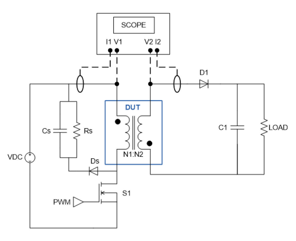
Applying the Proposed Calculation Method to Flyback Transformers

A way to “extend” the proposed method to flyback transformers is the calculation of the loss in each winding separately at each frequency point. For instance, consider the case of Figure 12. During T1, when the primary winding (W₁) is conducting I₁, the power loss can be found by evaluating the proximity loss (external fields) in W₁ and the secondary winding W₂ plus the skin effect contribution in W₁. Since W₂ is not conducting, it has no skin effect contribution in the loss during this state. The same occurs during T2, where W₁ is not conducting and W₂ is carrying I₂. In this state, the loss is the contribution of the proximity field in W₁ and W₂ plus the skin contribution only in W₂. Then, the total loss is the sum of P₁ and P₂ (15).

$$P_1=P_{Prox1}+P_{Prox2}+P_{Skin1}$$

(13)

$$P_2=P_{Prox1}+P_{Prox2}+P_{Skin2}$$

(14)

$$P_{Total}=P_1+P_2$$

(15)

This is no different than the application in power inductors; in fact, it is just the same as applying the method in two inductors (but considering the losses due to eddy currents in the additional nonexcited conductors). Nevertheless, this approach is not valid because the currents in the primary and the secondary do not have infinite di/dt, and thus, there is some time during the transitions where the conduction is overlapped and the coupling between windings should be considered [39].

A way to consider this in the calculations is by means of analysis in the frequency domain (this means that the currents through the windings are considered to be flowing simultaneously). This is, as usual, carried out through the harmonic decomposition of the currents in the windings and calculating the proximity loss, as well as the skin loss, at any frequency point by means of the calculation of the fields according to the corresponding values of the primary and secondary currents at the same time. This way, the fringing field source, H_g, can be assumed as the same for both windings, since N₁I₁ = N₂I₂ and is calculated according to the peak value of the current at the considered harmonic (using either I₁ or I₂ for the calculation of H_g). The proximity field, H_p, is calculated considering the currents through each conductor (I₁ or I₂ for primary or secondary turns, respectively).

A comparison against measurements on a flyback converter prototype was performed. Three different transformers were built and used in the flyback prototype. The characteristics of the transformers, as well as the operating conditions and measurements in the converter are stated in

Table 2. Characteristics of the measured transformers.

Component	Core Material	Gap Length (mm)	Turns/Parallel
			Primary	Secondary
T1	RM8/I 3F3	0.40	20/1 AWG23	3/3 AWG23
T2	RM8/I 3F3	0.72	26/1 AWG25	4/3 AWG25
T3	RM10 N41	0.44	12/1 AWG23	2/3 AWG19

,

Table 3. Measured operating conditions in the flyback converter prototype.

DUT	Duty Cycle (%)	INPUT		OUTPUT		Temperature (°C)
		Voltage (V)	Current (A)	Voltage (V)	Current * (A)	MOSFET	DIODE	R Snubber	D Snubber
T1	50	40.45	0.80	1.75	3.09	113.2	61.0	104.4	46.8
	50	28.30	0.60	1.26	2.23	56.5	52.8	70.7	39.4
	15	48.15	0.06	1.16	0.52	32.0	34.1	37.3	31.8
T2	50	39.20	0.79	2.20	2.86	99.0	59.0	98.8	43.9
	50	27.11	0.58	1.56	2.03	53.7	51.0	65.4	38.6
	15	48.20	0.06	1.22	0.56	31.0	34.0	36.5	30.6
T3	50	28.00	0.78	1.10	1.95	141.8	50.2	77.7	38.2
	15	48.13	0.11	0.86	1.02	33.8	39.2	45.2	31.5

* Current through the resistive load at the output.

, and

Table 4. Measured values in the flyback converter prototype.

DUT	Input Power (W)	Output Power (W)	Clamping Loss (W)	MOSFET Loss (W)	Diode Loss (W)	Calculated Core Loss (W)	Measured Winding Loss (W)	Calculated Winding Loss (W) Proposed Skin Depth
T1	32.36	5.41	14.77	5.88	1.29	4.40	0.62	0.60	0.18
	16.98	2.81	7.63	1.85	0.85	3.48	0.37	0.32	0.10
	2.70	0.60	1.49	0.12	0.16	0.29	0.03	0.03	0.01
T2	30.97	6.29	14.64	4.89	1.18	2.92	1.04	1.03	0.32
	15.72	3.17	7.54	1.59	0.94	1.93	0.56	0.54	0.18
	2.84	0.69	1.49	0.10	0.16	0.35	0.07	0.06	0.01
T3	21.84	2.15	9.53	8.03	0.83	0.71	0.59	0.56	0.09
	5.44	0.88	2.99	0.18	0.37	0.88	0.13	0.13	0.02

, respectively. The duty cycle was fixed (around 15% and 50%) in all tests and is also specified in the operating condition in Table 3. The calculated results are compared with the measured values in Table 4.

The flyback prototype and the measurement setup can be seen in Figure 13 and Figure 14. The measurement procedure followed is summarized below:

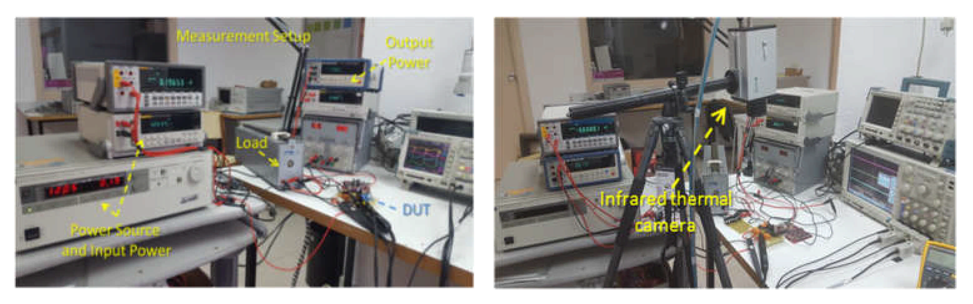
• For a given operating point in the converter, the input and output power were measured using precision meters, while an infrared camera was used to register the temperature of the semiconductors (main switch, the clamping diode, and output diode) and the clamping resistor. The total loss in the converter is the difference between the measured input and output power;
• Since a regulated source was used for the input voltage, no input capacitor was used in order to avoid additional loss due to the corresponding ESR. Furthermore, the required output capacitance, as well as the clamping capacitance were obtained by stacking a big number of parallel capacitors (in order to reduce, and neglect, the power loss due to the corresponding ESR);
• The semiconductors and clamping resistor were later characterized in order to subtract their respective losses from the measured values. To do this, the information taken from the thermal monitor was used to characterize the components by means of the association of a specific power loss with a given temperature (which corresponds to the considered operating point). This was performed by pushing a controlled DC current through the device to make it reach the same temperature that was observed during operation;
• Then, the power loss in the transformer (which includes the core loss) was assumed to be the difference between the total power loss and losses in the semiconductors and clamping circuit;
• The core loss was later taken out from the obtained value by means of the subtraction of an analytically calculated core loss (using the iGSE described in [40]), by means of (16), where k, α, and β are the Steinmetz parameters of the used magnetic materials (from datasheet). The waveform of the flux density was determined according to the measured currents, or voltages, in the transformer;
• Finally, the measured winding loss is the total difference among the input power, output power, losses in the devices, and the calculated core loss of the transformer (18).

$${\overline{P}}_v=\frac{1}{T}{{\displaystyle \int }}_0^T{k}_i{\left|\frac{dB}{dt}\right|}^{\alpha }{\left(∆B\right)}^{\beta -\alpha }dt$$

(16)

$$k_i=\frac{k}{{\left(2\pi \right)}^{\alpha -1}{{\displaystyle \int }}_0^{2\pi }{\left|\cos \theta \right|}^{\alpha }{2}^{\beta -\alpha }d\theta }$$

(17)

$$P_{winding}=P_{in}-P_{out}-P_{devices}-P_{core}$$

(18)

6. Conclusions

An analytical method to calculate winding loss in gapped magnetic components was proposed in this paper. Several expressions of the state-of-the-art were combined into a new method to obtain the total 2D losses in the windings of the magnetic component. The proposed method was based on a simple calculation of the proximity field combined with the Bessel function approach for the calculation of the power loss in each conductor. The calculated results by means of the application of the proposed method in several components were very close to the FEA calculations and measurements (from which the validity of the model can be derived).

The presented method has two important limitations that need to be considered: First, Expressions (6) and (7), which were used to calculate the fringing field due to the air gap at a given position of the window breath, are limited to components with a symmetric gap with respect to its core. This means that they can only be used in concentric geometries with a central air gap placed in its central leg (such as RM-, EE-, and ETD-like structures). This approach, however, could be extended to components with a distributed air gap as long as its position remains symmetric with respect to the core. In this case, H_g and H_g’, which are the magnitude of the reference sources (in the central and external legs) of the fringing field, must be calculated in a different way (for instance, using a reluctance model). Second, since it is a simplified method, where the fringing and proximity fields are considered to be “static and independent” and are calculated separately, an error, especially at high frequencies, is introduced in the calculation of the fields and, thus, in the calculation of the losses. Moreover, the main equation, which uses Bessel functions, which are not very accurate at high frequencies when applied to closely packed windings, Expression (1), which is valid for a homogeneous magnetic field, is used in an application where the external field is not uniform, and this is, also, a source of errors in the estimations. The quantification of this limitation can be seen in Figure 4, Figure 6, Figure 10 and Figure 11, where the difference with respect to FEM calculations can be appreciated as the frequency increases.

Even with those limitations in the accuracy, the obtained results, compared with FEA and measurements, were very good, especially in the low–medium-frequency range, and the method can be integrated into design and optimization tools in order to evaluate the influence of the gap in the windings from the early stages of the design process.

Furthermore, it is important to mention that the power loss must be evaluated in every single turn of the winding, which means that in components with a high number of turns, the required calculation time can be significant. This does not mean that an excessive calculation time is needed to apply the method; in fact, with an average computer, for example, the computation time for a 60-turn inductor was around 30 ms, which is much faster than FEA on the same computer (around 7 s, excluding the required modeling time). In low-frequency applications, as the calculation of the proximity field represents an important effort in terms of computing time [20], the influence of the near conductors over the winding loss can be neglected and the total losses in the winding can be calculated as the sum of (5) and (8), multiplied by the square of the RMS current through the winding, without a significant reduction of the accuracy.

References

1. Dowell, P. Effects of eddy currents in transformer windings. Proc. Inst. Electr. Eng. 1966, 113, 1387–1394. [Google Scholar] [CrossRef]
2. Nan, X.; Sullivan, C.R. An improved calculation of proximity-effect loss in high-frequency windings of round conductors. In Proceedings of the IEEE 34th Annual Conference on Power Electronics Specialist, 2003. PESC ’03, Acapulco, Mexico, 15–19 June 2003; Institute of Electrical and Electronics Engineers: New York, NY, USA, 2003; Volume 2, pp. 853–860. [Google Scholar]
3. Nan, X.; Sullivan, C.R. Simplified high-accuracy calculation of eddy-current loss in round-wire windings. In Proceedings of the 2004 IEEE 35th Annual Power Electronics Specialists Conference (IEEE Cat. No. 04CH37551), Aachen, Germany, 20–25 June 2004; Institute of Electrical and Electronics Engineers: New York, NY, USA, 2004; Volume 2, pp. 873–879. [Google Scholar]
4. Ferreira, J. Improved analytical modeling of conductive losses in magnetic components. IEEE Trans. Power Electron. 1994, 9, 127–131. [Google Scholar] [CrossRef]
5. Robert, F.; Mathys, P.; Schauwers, J.-P. A closed-form formula for 2-D ohmic losses calculation in SMPS transformer foils. IEEE Trans. Power Electron. 2001, 16, 437–444. [Google Scholar] [CrossRef]
6. Holguin, F.A.; Asensi, R.; Prieto, R.; Cobos, J.A. Simple analytical approach for the calculation of winding resistance in gapped magnetic components. In Proceedings of the 2014 IEEE Applied Power Electronics Conference and Exposition—APEC 2014, Fort Worth, TX, USA, 16–20 March 2014; Institute of Electrical and Electronics Engineers: New York, NY, USA, 2014; pp. 2609–2614. [Google Scholar]
7. Bahmani, M.A.; Thiringer, T.; Ortega, H. An accurate pseudoempirical model of winding loss calculation in HF foil and round conductors in Switchmode magnetics. IEEE Trans. Power Electron. 2014, 29, 4231–4246. [Google Scholar] [CrossRef]
8. Severns, R. Additional losses in high frequency magnetics due to non ideal field distributions. In Proceedings of the APEC ’92 Seventh Annual Applied Power Electronics Conference and Exposition, Boston, MA, USA, 23–27 February 1992; Institute of Electrical and Electronics Engineers: New York, NY, USA, 2003; pp. 333–338. [Google Scholar]
9. Mao, X.; Chen, W.; Li, Y. Winding loss mechanism analysis and design for new structure high-frequency gapped inductor. IEEE Trans. Magn. 2005, 41, 4036–4038. [Google Scholar]
10. Asensi, R.; Cobos, J.A.; García, O.; Prieto, R.; Uceda, J. A full procedure to model high frequency transformer windings. In Proceedings of the 25th Annual IEEE Power Electronics Specialists Conference, Taipei, Taiwan, 20–25 June 1994; Volume 2, pp. 856–863. [Google Scholar]
11. Asensi, R.; Prieto, R.; Cobos, J.A.; Uceda, J. Modelling high-frequency multiwinding magnetic components using fi-nite-element analysis. IEEE Trans. Magn. 2007, 43, 3840–3850. [Google Scholar] [CrossRef]
12. Prieto, R.; Asensi, R.; Fernandez, C.; Oliver, J.A.; Cobos, J.A. Bridging the gap between FEA field solution and the magnetic component model. IEEE Trans. Power Electron. 2007, 22, 943–951. [Google Scholar] [CrossRef]
13. Prieto, R.; Cobos, J.A.; García, O.; Alou, P.; Uceda, J. Study of 3-D magnetic components by means of double 2-D methodology. IEEE Trans. Ind. Electron. 2003, 50, 183–192. [Google Scholar] [CrossRef]
14. Prieto, R.; Oliver, J.; Cobos, J. Study of non-axisymmetric magnetic components by means of 2D FEA solvers. In Proceedings of the 2005 IEEE 36th Power Electronics Specialists Conference, Recife, Brazil, 12–16 June 2005; pp. 1074–1079. [Google Scholar] [CrossRef]
15. Van den Bossche, A.; Valchev, V.C. Taylor and francis. In Inductors and Transformers for Power Electronics; CRC Press: Boca Raton, FL, USA, 2005. [Google Scholar]
16. Snelling, E.C. Soft Ferrites, Properties and Applications, 2nd ed.; Butterworths: London, UK, 1988. [Google Scholar]
17. Roshen, W.A. Fringing field formulas and winding loss due to an air gap. IEEE Trans. Magn. 2007, 43, 3387–3394. [Google Scholar] [CrossRef]
18. Wei, C.; Xiaosheng, H.; Juanjuan, Z. Improved winding loss theoratical calculation of magnetic component with air gap. In Proceedings of the 7th International Power Electronics and Motion Control Conference, Harbin, China, 2–5 June 2012; Volume 1, pp. 471–475. [Google Scholar]
19. Hu, J.; Sullivan, C.R. Optimization of shapes for round-wire high-frequency gapped-inductor windings. In Proceedings of the Conference Record of 1998 IEEE Industry Applications Conference. Thirty-Third IAS Annual Meeting (Cat. No.98CH36242), St. Louis, MO, USA, 12–15 October 1998; Institute of Electrical and Electronics Engineers: New York, NY, USA, 2002; Volume 2, pp. 907–912. [Google Scholar]
20. Leuenberger, D.; Biela, J. Semi-numerical method for loss-calculation in foil-windings exposed to an air-gap field. In Proceedings of the 2014 International Power Electronics Conference (IPEC-Hiroshima 2014—ECCE ASIA), Hiroshima, Japan, 18–21 May 2014; Institute of Electrical and Electronics Engineers: New York, NY, USA, 2014; pp. 868–875. [Google Scholar]
21. Albach, M.; Rossmanith, H. The influence of air gap size and winding position on the proximity losses in high frequency transformers. In Proceedings of the 2001 IEEE 32nd Annual Power Electronics Specialists Conference (IEEE Cat. No.01CH37230), Vancouver, BC, Canada, 17–21 June 2001; Institute of Electrical and Electronics Engineers: New York, NY, USA, 2002; Volume 3, pp. 1485–1490. [Google Scholar]
22. Albach, M. Two-dimensional calculation of winding losses in transformers. In Proceedings of the 2000 IEEE 31st Annual Power Electronics Specialists Conference. Conference Proceedings (Cat. No.00CH37018), Galway, Ireland, 23 June 2000; Institute of Electrical and Electronics Engineers: New York, NY, USA, 2002; Volume 3, pp. 1639–1644. [Google Scholar]
23. Sullivan, C.R. Computationally efficient winding loss calculation with multiple windings, arbitrary waveforms, and two-dimensional or three-dimensional field geometry. IEEE Trans. Power Electron. 2001, 16, 142–150. [Google Scholar] [CrossRef] [Green Version]
24. Zimmanck, D.R.; Sullivan, C.R. Efficient calculation of winding-loss resistance matrices for magnetic components. In Proceedings of the 2010 IEEE 12th Workshop on Control and Modeling for Power Electronics (COMPEL), Boulder, CO, USA, 28–30 June 2010; pp. 1–5. [Google Scholar] [CrossRef]
25. Acero, J.A.; Hernandez, P.; Burdio, J.; Alonso, R.; Barragdan, L. Simple resistance calculation in litz-wire planar windings for induction cooking appliances. IEEE Trans. Magn. 2005, 41, 1280–1288. [Google Scholar] [CrossRef]
26. Lope, I.; Acero, J.; Burdío, J.M.; Carretero, C.; Alonzo, R. Design and implementation of PCB inductors with litz-wire structure for conventional-size large-signal domestic induction heating applications. IEEE Trans. Ind. Appl. 2015, 51, 2434–2442. [Google Scholar] [CrossRef]
27. Lope, I.; Carretero, C.; Acero, J.A.; Alonso, R.; Burdio, J.M. Frequency-dependent resistance of planar coils in printed circuit board with litz structure. IEEE Trans. Magn. 2014, 50, 1–9. [Google Scholar] [CrossRef]
28. Acero, J.A.; Burdio, J.; Barragan, L.; Puyal, D.; Alonso, R. Frequency-dependent resistance in Litz-wire planar windings for all-metal domestic induction heating appliances. In Proceedings of the Twentieth Annual IEEE Applied Power Electronics Conference and Exposition, 2005, APEC 2005, Austin, TX, USA, 6–10 March 2005; Volume 2, p. 1294. [Google Scholar] [CrossRef]
29. Wallmeier, P.; Frohleke, N.; Grotstollen, H. Improved analytical modeling of conductive losses in gapped high-frequency inductors. In Proceedings of the Conference Record of 1998 IEEE Industry Applications Conference. Thirty-Third IAS Annual Meeting (Cat. No.98CH36242), The 1998 IEEE Industry Applications Conference, St. Louis, MO, USA, 12–15 October 1998; Institute of Electrical and Electronics Engineers: New York, NY, USA, 2002; Volume 37, pp. 1045–1054. [Google Scholar] [CrossRef]
30. Lammeraner, J.; Stalf, M. Eddy Currents; ILIFFE books LTD.: London, UK, 1966. [Google Scholar]
31. Albach, M.; Stadler, A.; Spang, M. The influence of ferrite characteristics on the inductance of coils with rod cores. IEEE Trans. Magn. 2007, 43, 2618–2620. [Google Scholar] [CrossRef]
32. Deng, Q.; Liu, J.; Czarkowski, D.; Kazimierczuk, M.K.; Bojarski, M.; Zhou, H.; Hu, W. Frequency-dependent resistance of litz-wire square solenoid coils and quality factor optimization for wireless power transfer. IEEE Trans. Ind. Electron. 2016, 63, 2825–2837. [Google Scholar] [CrossRef]
33. Podoltsev, A.; Kucheryavaya, I.; Lebedev, B.; Podoltsev, A.; Kucheryavaya, I.; Lebedev, B. Analysis of effective resistance and eddy-current losses in multiturn winding of high-frequency magnetic components. IEEE Trans. Magn. 2003, 39, 539–548. [Google Scholar] [CrossRef]
34. Etemadrezaei, M.; Lukic, S.M. Equivalent complex permeability and conductivity of Litz wire in wireless power transfer systems. In Proceedings of the 2012 IEEE Energy Conversion Congress and Exposition (ECCE), Raleigh, NC, USA, 15–20 September 2012; pp. 3833–3840. [Google Scholar] [CrossRef]
35. Stadler, A.; Huber, R.; Stolzke, T.; Gulden, C. Analytical calculation of copper losses in Litz-Wire windings of gapped inductors. IEEE Trans. Magn. 2014, 50, 81–84. [Google Scholar] [CrossRef]
36. Meeker, D.C.; Meeker, D.C. An improved continuum skin and proximity effect model for hexagonally packed wires. J. Comput. Appl. Math. 2012, 236, 4635–4644. [Google Scholar] [CrossRef] [Green Version]
37. Stadler, A. The optimization of high frequency inductors with litz-wire windings. In Proceedings of the 2013 International Conference-Workshop Compatibility and Power Electronics, Ljubljana, Slovenia, 5–7 June 2013; Institute of Electrical and Electronics Engineers: New York, NY, USA, 2013; pp. 209–213. [Google Scholar]
38. Gyselinck, J.; Dular, P. Frequency-domain homogenization of bundles of wires in 2-D magneto-dynamic FE calculations. IEEE Trans. Magn. 2005, 41, 1416–1419. [Google Scholar] [CrossRef] [Green Version]
39. Spreen, J. Electrical terminal representation of conductor loss in transformers. IEEE Trans. Power Electron. 1990, 5, 424–429. [Google Scholar] [CrossRef]
40. Venkatachalam, K.; Sullivan, C.R.; Abdallah, T.; Tacca, H. Accurate prediction of ferrite core loss with nonsinusoidal waveforms using only Steinmetz parameters. In Proceedings of the 2002 IEEE Workshop on Computers in Power Electronics, Mayaguez, PR, USA, 3–4 June 2002; pp. 36–41. [Google Scholar]
Figure 1. (a) Axisymmetric representation of a magnetic component with 13 turns (0.6 mm in diameter and a separation between turns of 0.1 mm); (b) the equivalent resistance vs. frequency in the component with an air gap (in the central leg) of 0.4 mm, calculated by means of Dowell’s equation and FEA.
Electronics 10 01683 g001
Figure 2. Representation of fringing and proximity ideal fields over a round conductor in a gapped magnetic component.
Electronics 10 01683 g002
Figure 3. (a) Representation of two neighbor conductors; (b) axisymmetric FEA setup for the proximity effect evaluation between adjacent round conductors (symmetry axis at x/2 in an air analysis space of 15 mm of radius with vector potential A = 0 in the outer edge).
Electronics 10 01683 g003
Figure 4. Normalized resistance of Conductor 1 as a function of the separation from Conductor 2 (center-to-center) at different frequencies.
Electronics 10 01683 g004
Figure 5. Axisymmetric representation (cylindrical coordinates) of AWG24 round conductors in an RM6 core with an air gap.
Electronics 10 01683 g005
Figure 6. Equivalent resistance vs. frequency for the cases (AE) described in Table 1.
Electronics 10 01683 g006
Figure 7. Axisymmetric representation of an RM6 core for the magnetostatic analysis. The case with 11 spaced conductors carrying a current of 1 A (NI/lg = 22 × 103 A/m) and the zone divisions for the representation of the accuracy of the calculated fields.
Electronics 10 01683 g007
Figure 8. Analytical and numerical contour plot of the magnetic field for the inductor in Figure 7.
Electronics 10 01683 g008
Figure 9. (a) Axisymmetric representation of the considered inductors. Representation of a 60 AWG24 turn inductor in an RM8/I core (15 turns per layer); (b) RM8/I-3F3 cores with air gaps of 0.4 mm, 0.72 mm, and 2.2 mm (from left to right); (c) windings of 15 to 60 turns (1 to 4 layers) with AWG24 round wire.
Electronics 10 01683 g009
Figure 10. Equivalent resistance vs. frequency of the inductors in Figure 9. Comparison of the analytical and FEA results for components with 1 to 4 layers (15 to 60 turns) with 0.4 mm, 0.72 mm, and 2.2 mm in (a), (b), and (c), respectively.
Electronics 10 01683 g010
Figure 11. Comparison of the calculated results (analytical and FEA compensated with a calculated core resistance) with measurements for components with 1 to 4 layers (15 to 60 turns) with 0.4 mm, 0.72 mm, and 2.2 mm in (a), (b), and (c), respectively.
Electronics 10 01683 g011
Figure 12. Currents through the windings of flyback transformers, time domain.
Electronics 10 01683 g012
Figure 13. Measurement setup scheme used for measuring winding loss in a flyback converter’s gapped transformer.
Electronics 10 01683 g013
Figure 14. Setup for the winding loss measurement in the flyback transformer.
Electronics 10 01683 g014