
Adaptive Data Length Method for GPS Signal Acquisition in Weak to Strong Fading Conditions

 , , ,
, , ,  and
and 
Abstract
:1. Introduction
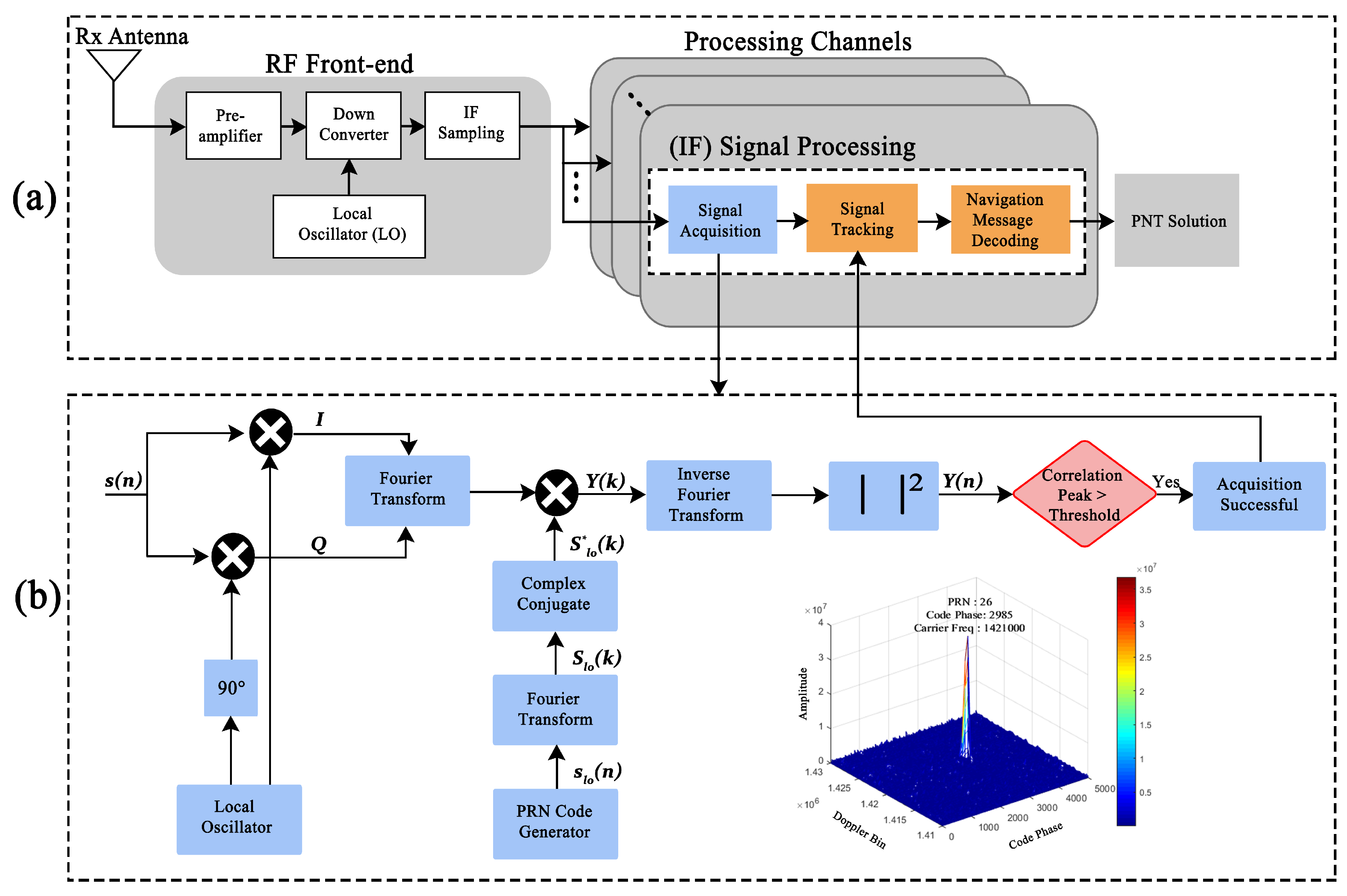
2. Signal Acquisition Methodology
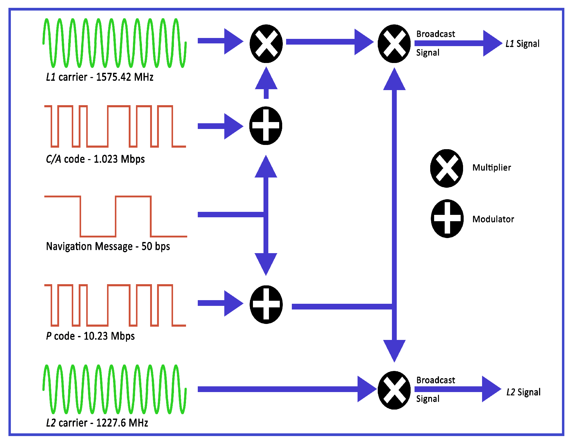
- : is the amplitude of the C/A code
- : is the C/A code of the satellite
- : is the navigation data bits having values
- : is the carrier frequency
- : is the Doppler shift
- : is the amplitude precise code or
- : is the precise code or
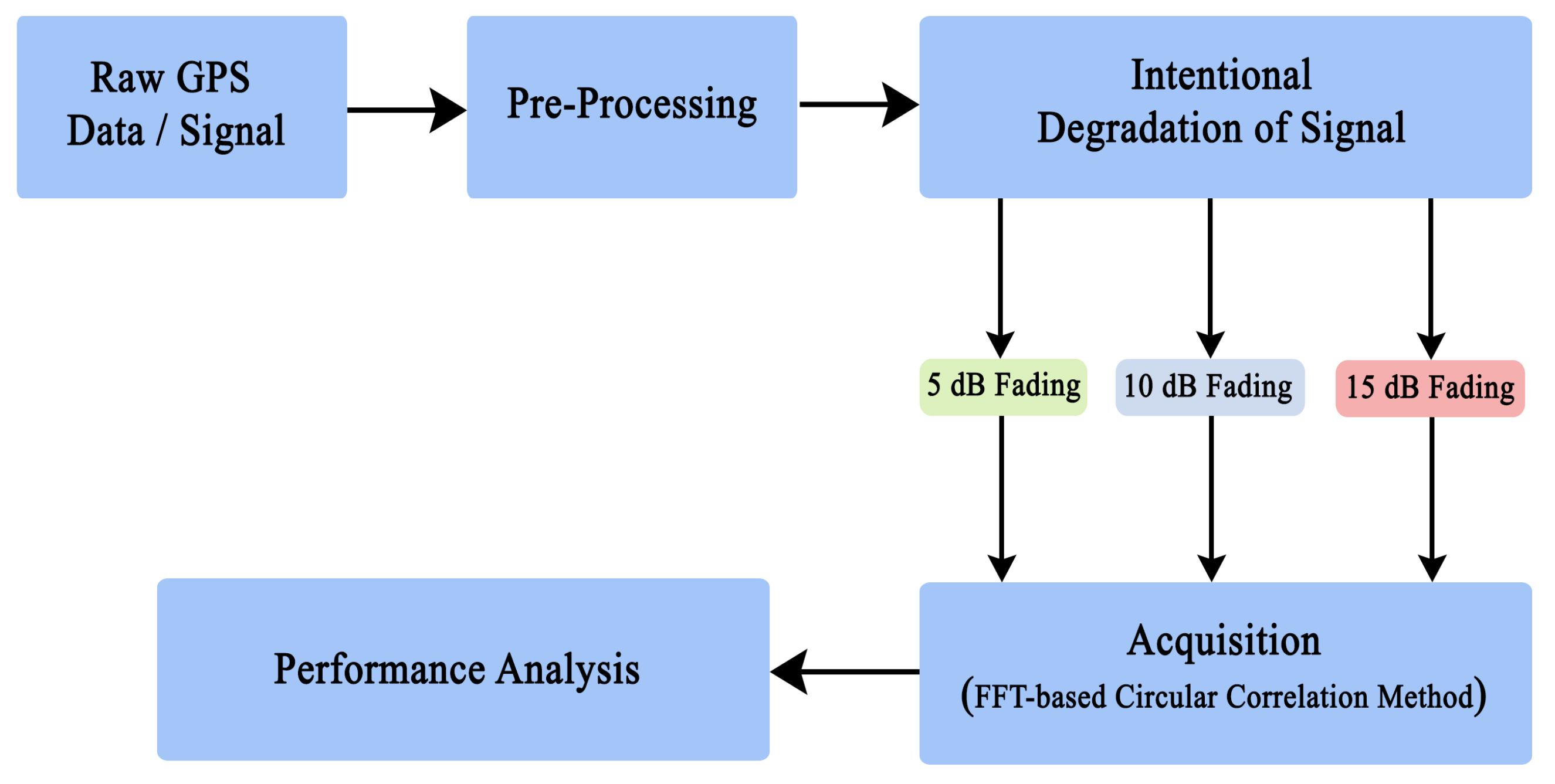
3. Methodology and Experimental Setup
4. Fading Effects on Acquisition and Signal Power Levels
5. Detection Performance
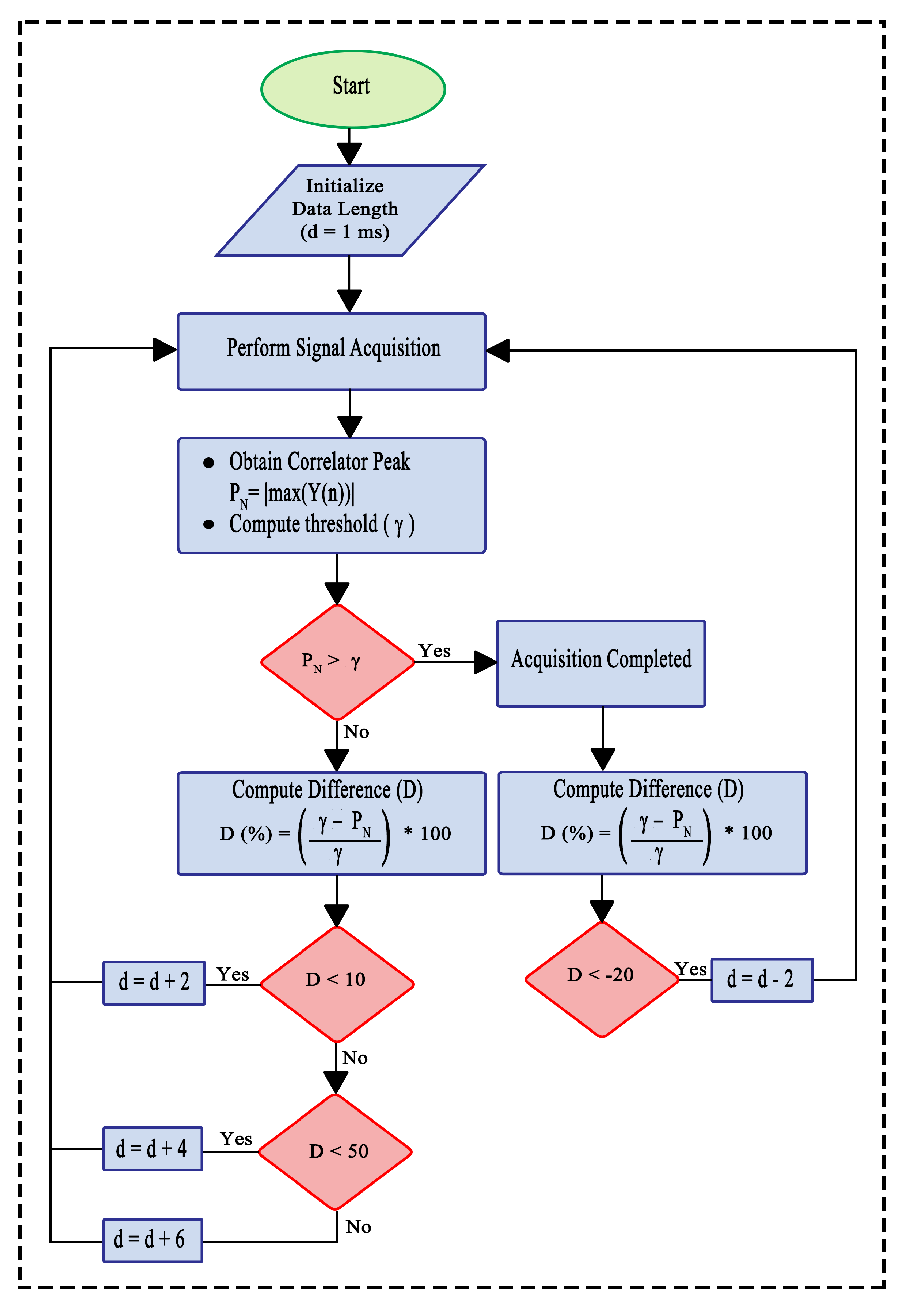
6. Adaptive Data Length (ADL) Method for Efficient Signal Acquisition
7. Conclusions
Author Contributions
Funding
Conflicts of Interest
References
- European Global Navigation Satellite Systems Agency (GSA). GNSS Market Report. Available online: https://www.gsa.europa.eu/market/market-report/ (accessed on 17 May 2021).
- Guo, J.; Li, X.; Li, Z.; Hu, L.; Yang, G.; Zhao, C.; Fairbairn, D.; Watson, D.; Ge, M. Multi-GNSS precise point positioning for precision agriculture. Precis. Agric. 2018, 19, 895–911. [Google Scholar] [CrossRef] [Green Version]
- Xu, G.; Xu, Y. GPS: Theory, Algorithms and Applications; Springer: Berlin/Heidelberg, Germany, 2016. [Google Scholar]
- Skog, I.; Handel, P. In-car positioning and navigation technologies—A survey. IEEE Trans. Intell. Transp. Syst. 2009, 10, 4–21. [Google Scholar] [CrossRef]
- Stallo, C.; Neri, A.; Salvatori, P.; Coluccia, A.; Capua, R.; Olivieri, G.; Gattuso, L.; Bonenberg, L.; Moore, T.; Rispoli, F. GNSS-based Location Determination System Architecture for Railway Performance Assessment in presence of local effects. In Proceedings of the 2018 IEEE/ION Position, Location and Navigation Symposium (PLANS), Monterey, CA, USA, 23–26 April 2018; pp. 374–381. [Google Scholar]
- El-Mowafy, A.; Kubo, N.; Kealy, A. Reliable Positioning and Journey Planning for Intelligent Transport Systems. Intell. Effic. Transp. Syst. Des. Model. Control. Simul. 2020, 41. [Google Scholar] [CrossRef] [Green Version]
- Ferreira, A.F.G.G.; Fernandes, D.M.A.; Catarino, A.P.; Monteiro, J.L. Localization and positioning systems for emergency responders: A survey. IEEE Commun. Surv. Tutor. 2017, 19, 2836–2870. [Google Scholar] [CrossRef]
- Joubert, N.; Reid, T.G.; Noble, F. Developments in Modern GNSS and Its Impact on Autonomous Vehicle Architectures. arXiv 2020, arXiv:2002.00339. [Google Scholar]
- Hein, G.W. Status, perspectives and trends of satellite navigation. Satell. Navig. 2020, 1, 1–12. [Google Scholar] [CrossRef]
- Hussain, A.; Ahmed, A.; Magsi, H.; Tiwari, R. Adaptive GNSS Receiver Design for Highly Dynamic Multipath Environments. IEEE Access 2020, 8, 172481–172497. [Google Scholar] [CrossRef]
- Tregoning, P.; Watson, C. Atmospheric effects and spurious signals in GPS analyses. J. Geophys. Res. Solid Earth 2009, 114. [Google Scholar] [CrossRef] [Green Version]
- Ahmed, A.; Tiwari, R.; Ali, S.I.; Jaffer, G. The Effects of Ionospheric Irregularities on the Navigational Receivers and Its Mitigation. In International Conference for Emerging Technologies in Computing; Springer: Berlin/Heidelberg, Germany, 2018; pp. 87–97. [Google Scholar]
- Seo, J.; Walter, T.; Enge, P. Availability Impact on GPS Aviation due to Strong Ionospheric Scintillation. IEEE Trans. Aerosp. Electron. Syst. 2011, 47, 1963–1973. [Google Scholar] [CrossRef]
- Brunner, F.K.; Welsch, W.M. Effect of the troposphere on GPS measurements. GPs World 1993, 4, 42. [Google Scholar]
- Zidan, J.; Adegoke, E.; Kampert, E.; Birrell, S.A.; Ford, C.R.; Higgins, M.D. GNSS vulnerabilities and existing solutions: A review of the literature. IEEE Access 2020. [Google Scholar] [CrossRef]
- Groves, P.D.; Jiang, Z.; Rudi, M.; Strode, P. A Portfolio Approach to NLOS and Multipath Mitigation in Dense Urban Areas; The Institute of Navigation: Manassas, VA, USA, 2013. [Google Scholar]
- Hsu, L.T. Analysis and modeling GPS NLOS effect in highly urbanized area. GPS Solut. 2018, 22, 1–12. [Google Scholar] [CrossRef] [Green Version]
- Pirsiavash, A.; Broumandan, A.; Lachapelle, G. Characterization of signal quality monitoring techniques for multipath detection in GNSS applications. Sensors 2017, 17, 1579. [Google Scholar] [CrossRef] [PubMed] [Green Version]
- Cheng, Q.; Chen, P.; Sun, R.; Wang, J.; Mao, Y.; Ochieng, W.Y. A New Faulty GNSS Measurement Detection and Exclusion Algorithm for Urban Vehicle Positioning. Remote Sens. 2021, 13, 2117. [Google Scholar] [CrossRef]
- Steven Miller, S.M.; Zhang, X.; Spanias, A. Multipath Effects in GPS Receivers: A Primer; Morgan and Claypool: San Rafael, CA, USA, 2015. [Google Scholar]
- Ioannides, R.T.; Pany, T.; Gibbons, G. Known vulnerabilities of global navigation satellite systems, status, and potential mitigation techniques. Proc. IEEE 2016, 104, 1174–1194. [Google Scholar] [CrossRef]
- Wang, Z.; Zhang, H.; Wang, M.; Liu, X.; Zhuang, Y.; Cai, H.; Yang, J.; Shi, L. Multi-Peak Double-Dwell GPS Weak Signal Acquisition Method and VLSI Implementation for Energy-Constrained Applications. Electronics 2018, 7, 31. [Google Scholar] [CrossRef] [Green Version]
- Rehman, M.U.; Gao, Y.; Chen, X.; Parini, C.G.; Ying, Z. Mobile terminal GPS antennas in multipath environment and effects of human body presence. In Proceedings of the 2009 Loughborough Antennas & Propagation Conference, Loughborough, UK, 16–17 November 2009; pp. 509–512. [Google Scholar]
- Betz, J.W. Navstar Global Positioning System. In Engineering Satellite-Based Navigation and Timing: Global Navigation Satellite Systems, Signals, and Receivers; Navstar: Reston, VA, USA, 2016; pp. 163–200. [Google Scholar] [CrossRef] [Green Version]
- Santerre, R.; Pan, L.; Cai, C.; Zhu, J. Single point positioning using GPS, GLONASS and BeiDou satellites. Positioning 2014, 5, 107–114. [Google Scholar] [CrossRef] [Green Version]
- Eissfeller, B.; Ameres, G.; Kropp, V.; Sanroma, D. Performance of GPS, GLONASS and Galileo. Photogramm. Week 2007, 7, 185–199. [Google Scholar]
- Tsui, J.B. Fundamentals of Global Positioning System Receivers: A Software Approach; John Wiley & Sons: Hoboken, NJ, USA, 2005; pp. 1–155. [Google Scholar]
- Kaplan, E.; Hegarty, C. Understanding GPS: Principles and Applications; Artech House: Boston, CA, USA, 2005. [Google Scholar]
- Borre, K.; Akos, D.M.; Bertelsen, N.; Rinder, P.; Jensen, S.H. A Software-Defined GPS and Galileo Receiver: A Single-Frequency Approach; Springer Science & Business Media: Berlin/Heidelberg, Germany, 2007. [Google Scholar]
- El-Bakry, H.M.; Mastorakis, N. Design of anti-GPS for reasons of security. CIS 2009, 9, 480–500. [Google Scholar]
- Alaqeeli, A.; Starzyk, J.; Van Graas, F. Real-time acquisition and tracking for GPS receivers. In Proceedings of the 2003 International Symposium on Circuits and Systems, ISCAS’03, Bangkok, Thailand, 25–28 May 2003; Volume 4, p. IV. [Google Scholar]
- Akopian, D. Fast FFT based GPS satellite acquisition methods. IEE Proc. Radar Sonar Navig. 2005, 152, 277–286. [Google Scholar] [CrossRef] [Green Version]
- Manandhar, D.; Suh, Y.; Shibasaki, R. GPS signal acquisition and tracking-An Approach towards development of Software-based GPS Receiver. Tech. Rep. IEICE 2004. Available online: https://www.semanticscholar.org/paper/GPS-Signal-Acquisition-and-Tracking-An-Approach-of-Manandhar-Sum/260d7fcd41d657fc67a014a89a163496ee465067/ (accessed on 14 February 2021).
- Ahamed, S.F.; Rao, G.S.; Ganesh, L. Fast Acquisition of GPS Signal using FFT Decomposition. Procedia Comput. Sci. 2016, 87, 190–197. [Google Scholar] [CrossRef] [Green Version]
- Cui, H.; Li, Z.; Dou, Z. Fast acquisition method of GPS signal based on FFT cyclic correlation. Int. J. Commun. Netw. Syst. Sci. 2017, 10, 246–254. [Google Scholar] [CrossRef] [Green Version]
- Lin, D.; Tsui, J. Acquisition schemes for software GPS receiver. In Proceedings of the 11th International Technical Meeting of the Satellite Division of the Institute of Navigation (ION GPS 1998), Nashville, TN, USA, 15–18 September 1998; Volume 11, pp. 317–326. [Google Scholar]
- Gao, F. Performance Analysis of Long-Time Coherent Integral Acquisition Algorithm for Weak GNSS Signals. IOP Conf. Ser. Earth Environ. Sci. 2020, 428, 012002. [Google Scholar] [CrossRef]
- Luo, Y.; Zhang, L.; Ruan, H. An Acquisition Algorithm Based on FRFT for Weak GNSS Signals in A Dynamic Environment. IEEE Commun. Lett. 2018, 22, 1212–1215. [Google Scholar] [CrossRef]
- Albuquerque, G.L.A.; Valderrama, C.; Silva, F.C.; Xavier-de-Souza, S. Time-effective GPS time domain signal Acquisition Algorithm. In Proceedings of the 2016 International Conference on Localization and GNSS (ICL-GNSS), Barcelona, Spain, 28–30 June 2016; pp. 1–6. [Google Scholar]
- Psiaki, M.L. Block acquisition of weak GPS signals in a software receiver. In ION GPS; Citeseer: University Park, PA, USA, 2001; Volume 2001, pp. 1–13. Available online: https://www.ion.org/publications/abstract.cfm?articleID=1960 (accessed on 5 March 2021).
- He, G.; Song, M.; He, X.; Hu, Y. GPS signal acquisition based on compressive sensing and modified greedy acquisition algorithm. IEEE Access 2019, 7, 40445–40453. [Google Scholar] [CrossRef]
- Ahmed, A.; Tiwari, R.; Strangeways, H.J.; Dlay, S.; Johnsen, M.G. Wavelet-based analogous phase scintillation index for high latitudes. Space Weather 2015, 13, 503–520. [Google Scholar] [CrossRef] [Green Version]
- Ahmed, A.; Tiwari, R.; Strangeways, H.; Boussakta, S. Software-based receiver approach for acquiring GPS signals using block repetition method. In Proceedings of the 2014 7th ESA Workshop on Satellite Navigation Technologies and European Workshop on GNSS Signals and Signal Processing (NAVITEC), Noordwijk, The Netherlands, 3–5 December 2014; pp. 1–7. [Google Scholar]
- Chibout, B.; Macabiau, C.; Escher, A.C.; Ries, L.; Issler, J.L.; Corazza, S.; Bousquet, M.O. Comparison of Acquisition Techniques for GNSS Signal Processing in Geostationary Orbit. In Proceedings of the 2007 National Technical Meeting of the Institute of Navigation, San Diego, CA, USA, 22–24 January 2007. [Google Scholar]
- Lin, D.M. Comparison of acquisition methods for software GPS receiver. In Proceedings of the ION GPS 2000, Salt Lake City, UT, USA, 19–22 September 2000; pp. 2385–2390. [Google Scholar]
- Li, S.; Yi, Q.; Shi, M.; Chen, Q. Highly sensitive weak signal acquisition method for GPS/compass. In Proceedings of the 2014 International Joint Conference on Neural Networks (IJCNN), Beijing, China, 6–11 July 2014; pp. 1245–1249. [Google Scholar]
- O’Driscoll, C.; Murphy, C.C. Performance analysis of an FFT based fast acquisition GPS receiver. In Proceedings of the ION National Technical Meeting, San Diego, CA, USA, 24–26 January 2005; pp. 1014–1025. [Google Scholar]
- Chen, X.; Xu, J.; Ye, T.; Li, S.C. FFT-Based Acquisition for Weak GPS Signals. Microelectron. Comput. 2010. Available online: https://citeseerx.ist.psu.edu/viewdoc/download?doi=10.1.1.725.7619&rep=rep1&type=pdf (accessed on 25 February 2021).
- Borio, D.; O’Driscoll, C.; Lachapelle, G. Coherent, noncoherent, and differentially coherent combining techniques for acquisition of new composite GNSS signals. IEEE Trans. Aerosp. Electron. Syst. 2009, 45, 1227–1240. [Google Scholar] [CrossRef]
- Ettus Research: A National Instruments Brand. USRP N210 Data Sheet. Available online: http://www.ti.com/lit/ds/symlink/cd4007ub.pdf (accessed on 13 May 2021).
- Tsui, J. Microwave Receivers with Electronic Warfare Applications; The Institution of Engineering and Technology: Raleigh, NC, USA, 2005. [Google Scholar]
- Skolnik, M.I. Introduction to Radar Systems; McGraw Hill Book Co.: New York, NY, USA, 1980; 590p. [Google Scholar]
- Zihuan, H.; Lei, Z. High-sensitive acquisition method of GPS signal based on iridium assistance. J. Eng. 2019, 2019, 6873–6875. [Google Scholar] [CrossRef]
- Bruyninx, C.; Aerts, W.; Legrand, J. Gps, Data Acquisition and Analysis. In Encyclopedia of Solid Earth Geophysics; Springer: Dordrecht, The Netherlands, 2011; pp. 420–431. [Google Scholar] [CrossRef]


| Acquisition Attempt | 1st Itr. d (ms) | D (%) | 2nd Itr. d (ms) | D (%) | 3rd Itr. d (ms) | D (%) | Remarks on Acquisition |
|---|---|---|---|---|---|---|---|
| 01 | 01 | 31.4 | 05 | −32 () | N/A | N/A | Acquisition declared in 2nd iteration using 5 ms of data |
| 02 | 01 | 30.8 | 05 | 43.5 | 09 | −85.7 () | Acquisition declared in 3rd iteration using 9 ms of data |
| 03 | 01 | 27.3 | 05 | −135 () | N/A | N/A | Acquisition declared in 2nd iteration using 5 ms of data |
| 04 | 01 | 34.0 | 05 | 32.1 | 09 | −5.3 () | Acquisition declared in 3rd iteration using 9 ms of data |
| 05 | 01 | 11.1 | 05 | −35.6 () | N/A | N/A | Acquisition declared in 2nd iteration using 5 ms of data |
| 06 | 01 | 37.3 | 05 | −36.5 () | N/A | N/A | Acquisition declared in 2nd iteration using 5 ms of data |
| 07 | 01 | 31.6 | 05 | 23.6 | 09 | −47.3 () | Acquisition declared in 3rd iteration using 9 ms of data |
| 08 | 01 | 28.9 | 05 | −17.8 () | N/A | N/A | Acquisition declared in 2nd iteration using 5 ms of data |
| 09 | 01 | 39.9 | 05 | 9.2 | 07 | −21.0 () | Acquisition declared in 3rd iteration using 7 ms of data |
| 10 | 01 | 52.6 | 07 | −5.8 () | N/A | N/A | Acquisition declared in 2nd iteration using 7 ms of data |
| Acquisition Attempt | 1st Itr. d (ms) | D (%) | 2nd Itr. d (ms) | D (%) | 3rd Itr. d (ms) | D (%) | 4th Itr. d (ms) | D (%) | 5th Itr. d (ms) | D (%) | Remarks on Acquisition |
|---|---|---|---|---|---|---|---|---|---|---|---|
| 01 | 01 | 54.9 | 07 | 11.2 | 11 | −10.31 () | N/A | N/A | N/A | N/A | Acquisition declared in 3rd iteration using 11 ms of data |
| 02 | 01 | 57.1 | 07 | 52.9 | 13 | 31.94 | 17 | −3.78 () | N/A | N/A | Acquisition declared in 4th iteration using 17 ms of data |
| 03 | 01 | 53.0 | 07 | 63.6 | 13 | 15.41 | 17 | −14.2 () | N/A | N/A | Acquisition declared in 4th iteration using 17 ms of data |
| 04 | 01 | 16.2 | 07 | 33.9 | 11 | 21.02 | 15 | −9.5 () | N/A | N/A | Acquisition declared in 4th iteration using 15 ms of data |
| 05 | 01 | 64.7 | 07 | 29.9 | 11 | 15.4 | 15 | 20.1 | 19 | −13.3 () | Acquisition declared in 5th iteration using 19 ms of data |
| 06 | 01 | 46.4 | 05 | 53.2 | 11 | 49.2 | 15 | 28.93 | 19 | 34.4 | Acquisition not declared in 2nd iteration using 5 ms of data |
| 07 | 01 | 66.2 | 07 | 45.8 | 11 | 52.01 | 17 | 7.82 | 19 | −3.7 () | Acquisition declared in 5th iteration using 19 ms of data |
| 08 | 01 | 63.3 | 07 | 28.3 | 11 | 27.32 | 15 | −12.36 () | N/A | N/A | Acquisition declared in 4th iteration using 15 ms of data |
| 09 | 01 | 51.5 | 05 | 16.5 | 11 | −2.71 () | N/A | N/A | N/A | N/A | Acquisition declared in 3rd iteration using 11 ms of data |
| 10 | 01 | 61.8 | 07 | 2.64 | 11 | 19.53 | 15 | 3.6 | 19 | −9.73 () | Acquisition declared in 5th iteration using 19 ms of data |
Publisher’s Note: MDPI stays neutral with regard to jurisdictional claims in published maps and institutional affiliations. |
© 2021 by the authors. Licensee MDPI, Basel, Switzerland. This article is an open access article distributed under the terms and conditions of the Creative Commons Attribution (CC BY) license (https://creativecommons.org/licenses/by/4.0/).
Share and Cite
Hussain, A.; Ahmed, A.; Magsi, H.; Soomro, J.B.; Bukhari, S.S.H.; Ro, J.-S. Adaptive Data Length Method for GPS Signal Acquisition in Weak to Strong Fading Conditions. Electronics 2021, 10, 1735. https://doi.org/10.3390/electronics10141735
Hussain A, Ahmed A, Magsi H, Soomro JB, Bukhari SSH, Ro J-S. Adaptive Data Length Method for GPS Signal Acquisition in Weak to Strong Fading Conditions. Electronics. 2021; 10(14):1735. https://doi.org/10.3390/electronics10141735
Chicago/Turabian StyleHussain, Arif, Arslan Ahmed, Hina Magsi, Jahangeer Badar Soomro, Syed Sabir Hussain Bukhari, and Jong-Suk Ro. 2021. "Adaptive Data Length Method for GPS Signal Acquisition in Weak to Strong Fading Conditions" Electronics 10, no. 14: 1735. https://doi.org/10.3390/electronics10141735
APA StyleHussain, A., Ahmed, A., Magsi, H., Soomro, J. B., Bukhari, S. S. H., & Ro, J.-S. (2021). Adaptive Data Length Method for GPS Signal Acquisition in Weak to Strong Fading Conditions. Electronics, 10(14), 1735. https://doi.org/10.3390/electronics10141735