Abstract
The flight trajectory of unmanned aerial vehicles (UAVs) can be significantly affected by external disturbances such as turbulence, upstream wake vortices, or wind gusts. These effects present challenges for UAV flight safety. Hence, addressing these challenges is of critical importance for the integration of unmanned aerial systems (UAS) into the National Airspace System (NAS), especially in terminal zones. This work presents a robust nonlinear control method that has been designed to achieve roll/yaw regulation in the presence of unmodeled external disturbances and system nonlinearities. The data from NASA-conducted airport experimental measurements as well as high-fidelity Large Eddy Simulations of the wake vortex are used in the study. Side-by-side simulation comparisons between the robust nonlinear control law and both linear and PID control laws are provided for completeness. These simulations are focused on applications involving small UAV affected by the wake vortex disturbance in the vicinity of the ground (which models the take-off or landing phase) as well as in the out-of-ground zone. The results demonstrate the capability of the proposed nonlinear controller to asymptotically reject wake vortex disturbance in the presence of the nonlinearities in the system (i.e., parametric variations, unmodeled, time-varying disturbances). Further, the nonlinear controller is designed with a computationally efficient structure without the need for the complex calculations or function approximators in the control loop. Such a structure is motivated by UAV applications where onboard computational resources are limited.
1. Introduction
The Federal Aviation Administration (FAA) currently faces numerous operational safety challenges associated with the integration of UAS flights in the NAS. For instance, the Integrated Safety Assessment Model (ISAM) [1] requires further development and improvements in order to adequately address UAS operations for current and future risk analyses. Motivated by the desire to improve the safety of UAS operating in the NAS, the development of novel UAV flight control technologies is of critical importance. Specifically, there is a need for control system technologies that are capable of quickly recovering from unpredictable and potentially hazardous operating conditions resulting from phenomena such as airflow disturbances due to upstream wake vortex, wind gusts, or turbulence. Based on these considerations, the focus of the current work is on the development of a nonlinear control method, which demonstrates a positive and accurate UAV trajectory regulation in the presence of wake vortex disturbance, in addition to the nonlinearity in the governing UAV dynamic model.
The UAV is a multi-input/multi-output (MIMO) system, which is a highly coupled and unstable system. A number of works are devoted to the problem of the UAV following the path in a windy environment [2,3] as well as in the presence of microburst [4]. Different control strategies have been widely used for the UAVs’ control, such as adaptive control [5,6,7], neural network-based [8,9] techniques, inversion techniques [10,11], optimal control [12,13], which may effectively compensate for the actuator nonlinearities. The linear quadratic regulator (LQR) [14,15] as well as robust [16,17,18] control methods have been used for lateral and longitudinal dynamics in flight control. However, such techniques require additional computational complexity over purely robust feedback designs. Hence, the minimalism of the controller design in this work is motivated by the desire to develop control methods that are suitable for small UAVs.
This work presents a robust nonlinear flight control strategy [19,20,21] capable of the uncertain bounded wake vortex disturbance rejection in different phases of evolution, including in-ground and out-of-ground effects. The control of the systems in the presence of uncertainties and unmodeled disturbances is used nowadays for various practical applications. For example, the robust control as well as station-keeping control of the underwater vehicle in the presence of the unmodeled disturbances and model uncertainties was applied by Vu et al. [22,23] to obtain the desired trajectory tracking performance of the AUV. Haitong Xu [24] recently demonstrated the control system for coupled path-following and the collision-avoided task of the ship model in the presence of static obstacles. The sliding mode control for second-order systems in application to UAVs for attitude and altitude control has been described [25,26]. The effective application of the robust control for the second order-systems [27,28] in the presence of the uncertain bounded disturbances was shown. The disturbance is modeled by applying the low-fidelity model of wake vortex pair [29,30] for the steady level flight and Monte-Carlo simulations scenario [31]. The high fidelity simulations (Large Eddy Simulation (LES)) of the wake vortex for the generator aircraft’s take-off and landing phases [32,33,34] are performed to model the in-ground phase of vortex evolution. Side-by-side simulations and performance comparisons with control method are provided for the robust nonlinear controller response at every flight phase. In addition, the comparison with the PID controller is demonstrated. The proposed control design is particularly advantageous in maintaining flight stability in the presence of a high degree of uncertainty and nonlinearity in the UAV operating conditions (e.g., flight conditions inherent in tight urban environments and terminal zones).
The remainder of this paper is organized as follows. The next three sections present the mathematical model utilized in the controller development as well as the nonlinear and linear controllers considered. Section 6 presents the wake vortex disturbance modeling methodology for low-fidelity and high-fidelity simulations. Finally, Section 7 outlines the numerical simulation and results, where the performance of the proposed controller is investigated and compared with the existing linear controllers.
2. Mathematical Model
This section describes the mathematical model utilized in controller development. The UAV dynamic model under consideration is assumed to contain parametric model uncertainty in addition to unmodeled, time-varying nonlinearities. The aircraft dynamics is modeled as a linear parameter-varying (LPV) system [35,36,37,38,39,40,41]:
where is a measurable parameter vector, called the scheduling parameter, are the deviation states, are the deviation inputs, are the deviation outputs, and is an unknown nonlinear disturbance. Here, represents the system matrix, the input matrix, the output matrix, and the feedthrough matrix. The system is then arranged such that
where , , , and are the known, nominal state space matrices. The parametric uncertainty is reflected by , and the structural knowledge about the uncertainty is contained in the matrices , , , and [42].
The lateral dynamics of an aircraft is described by the state vector with input vector , where v,p,r,, is lateral velocity, roll, and yaw rates and angles. The input parameters are aileron and rudder deflections. The maximum rate of deflection of ailerons and rudder is set to 30 deg/s, and the maximum amplitude is 25 deg. The scheduling parameter can be the altitude and Mach number, and the unknown disturbance could be wake vortex, wind gusts, turbulent disturbances, or nonlinearities not captured in the linear model.
Assumptions
- Assumption 1: We assume that the lateral dynamics is uncoupled from the longitudinal.
- Assumption 2: It is assumed that the magnitude of the wake vortex disturbance is bounded.
3. Nonlinear Robust Control
3.1. Control Objective
The control objective is to force the UAV attitude (i.e., and ) to regulate to a given constant value. To quantify the control objective, the trajectory regulation error and the auxiliary regulation error are defined as:
In Equation (7), denote positive, constant control gains. Thus, the trajectory regulation control objective can be stated mathematically as , where denotes the standard Euclidean norm of the vector argument. Note that, based on the auxiliary regulation error definitions in Equation (7), .
Note that the regulation error and auxiliary errors defined in Equations (6) and (7) are key in the contribution in the current study. The definitions of the auxiliary regulation errors enable us to recast the dynamic model in Equation (1) in a form that is amenable to roll/yaw angle angle regulation control. Indeed, it can be seen that the differentiation of produces a set of equations that render the roll and yaw angles (, ) fully controllable through the aileron and rudder deflections , . Thus, the auxiliary error terms , can be viewed as sliding surfaces, which enables us to prove our roll and yaw angle regulation results.
3.2. Robust Controller Development
In order to achieve asymptotic convergence of , to zero with a given convergence rate in the presence of a bounded disturbance (i.e., wake vortex or wind gust), we have to drive the auxiliary regulation error r to zero in finite time. Taking into account the original dynamic model and the auxiliary regulation error r, the auxiliary control term u is designed as:
where denotes a constant auxiliary matrix, and denotes the inverse of a matrix. The feedback control gains (i.e., amplifiers) ,, ,,, can be tuned to adjust the closed loop regulation response to achieve the desired system performance (e.g., to achieve a faster response time).
Note that the robust nonlinear control law given by Equation (8) ensures asymptotic trajectory regulation in the sense that
provided the control gains and introduced in Equation (8) are selected sufficiently large, and and are selected based on the known upper bounds on the disturbance (i.e., the known maximum velocity and acceleration of the wind gust).
A straightforward proof of the above statement based on Lyapunov stability analysis can be utilized and is omitted here for brevity. Details of the proof are similar to those provided in our recent results [19,20].
3.3. Observer Design
The control design presented in the current result is based on the assumption that only attitude measurements (i.e., and ) are available for feedback. Considering this, an observer (or estimator) will be employed, which estimates the complete system state using only the available attitude measurements. This section summarizes the design of the observer.
In Equation (1), the explicitly defined output y can be denoted as the sufficiently differentiable vector function . To facilitate the subsequent observer design and analysis, a vector of output derivatives is defined as:
where denotes the i-th Lie derivative of the output function along the direction of the vector field .
An observer that estimates the full state of the system in Equation (1) using only measurements of can be designed as [21]:
In Equation (11), is defined via the recursive form for . Furthermore, in Equation (11), denotes a diagonal matrix with positive elements defined as:
where , .
Similar to the design in [43], it can be shown that the observer design in Equation (11) achieves finite-time estimation of the state . Specifically, it can be shown that, through judicious selection of the diagonal matrix , for any . By including the additional term in the observer design, it follows that, for , the system converges to the sliding manifold , and the observer Equation (11) exactly estimates the state of the dynamic system in Equation (1).
4. Linear Controller
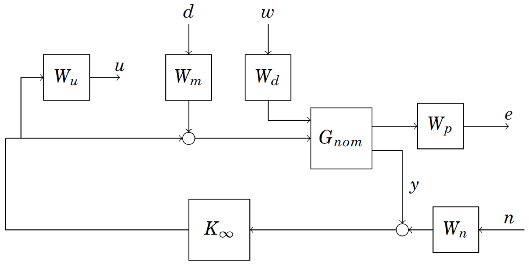
The interconnection used to synthesize the linear controllers is depicted in Figure 1. Here, e represents the control objective outputs, i.e., the measurable attitude outputs and . The controller takes the estimated state vector as feedback measurements. The objective is to minimize the -norm between the disturbances and wind gust and the lateral attitude and control action while compensating for model uncertainty.
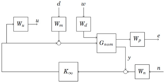
Figure 1.
Control interconnection for the linear design.
The performance specifications in Figure 1 are in the form of closed-loop transfer functions designed to be small through feedback. With this, the mathematical objective is to drive the -norm of the closed-loop transfer function, , to be less than 1. Hence, the design task is to find the appropriate weighting functions to meet the performance objectives. For this control design, the closed-loop transfer functions of the aircraft are
with
where is the output sensitivity transfer function, and is the complementary output sensitivity transfer function. Here, corresponds to the vehicle dynamics with sensor outputs, and are the vehicle dynamics used for wind and external disturbances. That is with
Constant weights, , are used to model the disturbances to each control input. This weight is selected as for all control inputs. Furthermore, a multiplicative input weight is included to avoid destabilizing unmodeled frequency modes outside the control bandwidth. The uncertainty model weight is described by .
On the other hand, the disturbance rejection of critical variables is enforced by a constant performance weight . A constant gain attenuation of is assigned to each control objective in order to ensure damping. Similarly, wind gust disturbances are attenuated with a constant weight , and noise is accounted for with the constant weight for each measurement. Once all the weights are defined, the next step is to find an optimal such that the system gain . The Robust Control Toolbox from MATLAB is used to design the controller with a system gain of . Hence, the designed controller achieves the control objectives specified in the control interconnection.
5. PID Controller
To provide a further comparison of the closed-loop system under wake vortex disturbances, the roll and yaw (i.e., and ) regulation control objective was tested using a PID controller. The Control Toolbox from MATLAB is used to design a PID controller. To adapt the Matlab PID controller simulation to our MIMO system, PID control laws are applied to each of the roll and yaw states separately. The parameters for proportional (P), integral (I) and derivative (D) gains, as well as filter coefficient (N) used in the transfer function for the PID controller Equation (16), are shown in Table 1. The Matlab “Transfer Function” tuning method was used to tune the controller.

Table 1.
PID control gains.
6. Wake Vortex Modeling
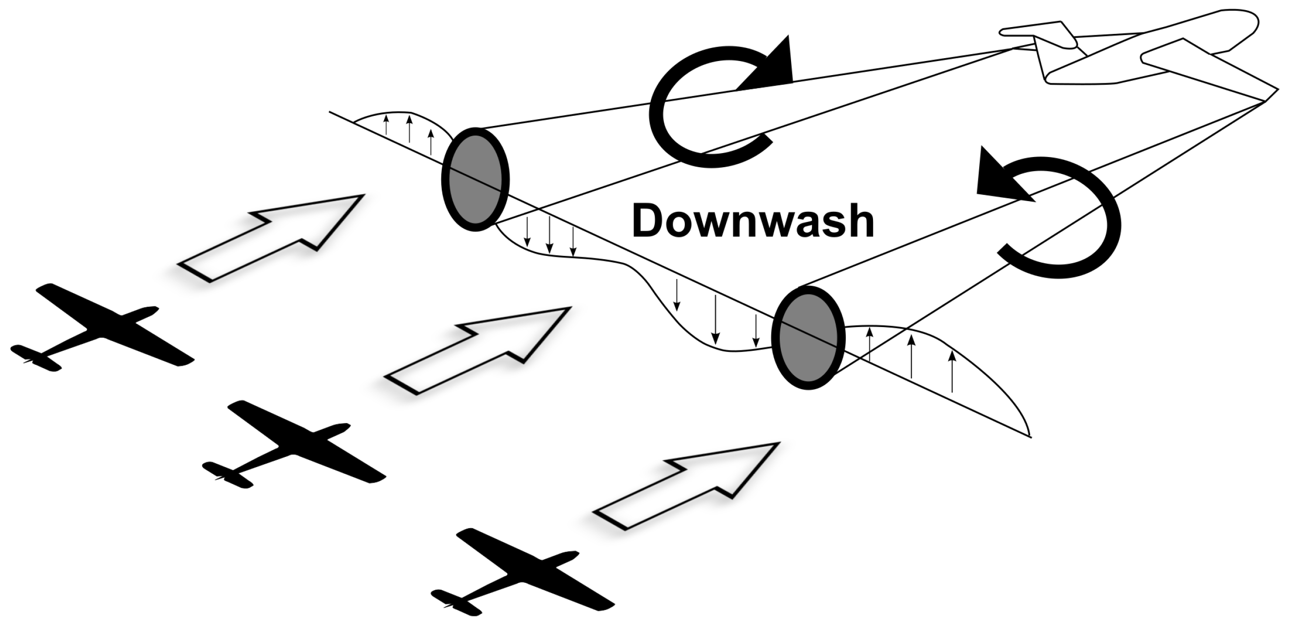
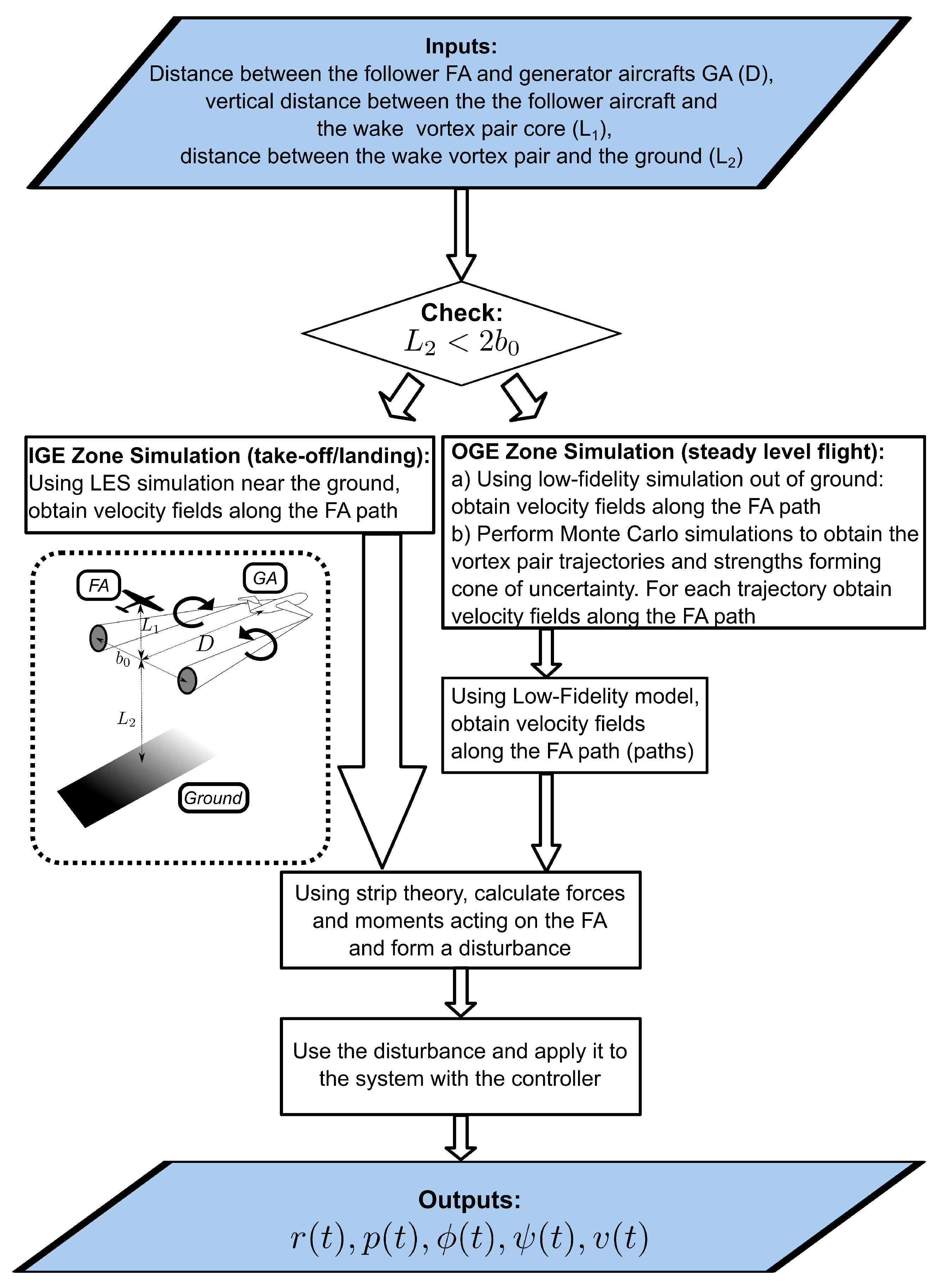
In order to determine the loads induced on the aircraft flying through the wake vortex, one needs to model the flow field induced by the vortex pair as well as the forces and moments acting on the airplane during the interaction. By the interaction, the authors mean the wake-vortex/aircraft contact when sweeping the follower aircraft (FA) through the wake in the direction perpendicular to the generator aircraft (GA) velocity vector, as shown in Figure 2. The general block diagram is shown in Figure 3. Knowing the wake characteristics of the generator aircraft with elliptically loaded wings, one can obtain the vortex flow field created by the vortex pair. The vortex pair in this study is modeled by Burnham–Hallock model [44] where tangential velocities induced by the wake are calculated with a constant core radius,

Figure 2.
Leader and follower aircraft schematics sweeping through the wake vortex.
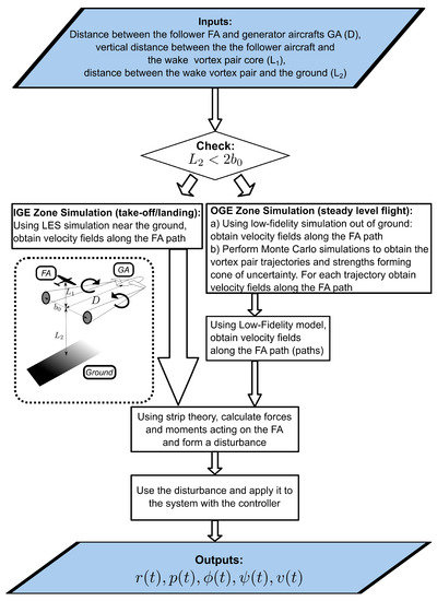
Figure 3.
Block diagram of the wake vortex/aircraft interaction simulation.
The evolution of the wake vortex was simulated by the Wake Vortex Safety System (WVSS) [45] in the out-of-ground effect zone (OGE) as well as in the in-ground effect zone (IGE), where the interaction of the wake vortex and surface boundary layer occurs. The forces and moments acting on the follower aircraft (FA) in both zones are calculated using the velocity field obtained from the simulations using the strip theory and form the disturbance (Equation (1)). In the rest of the paper, the steady level flight regime denotes the wake vortex/aircraft interaction in the OGE zone, and take-off/landing regime describes the interaction in the IGE zone.
Furthermore, Monte-Carlo simulations for the steady-level flight regime are performed for the OGE zone. Based on the data from NASA-conducted airport experimental measurements, the real cone of uncertainty of the wake vortex pair evolution (position and strength) was modeled using the WVSS. Thus, the controller performance was investigated within the experiment-based cone of uncertainty. The controller ability to withstand the wake vortex induced disturbances within the terminal zone was demonstrated. The full procedure of the Monte-Carlo approach and validation with the experimental data is discussed in our previous work [31]. Hence, the steady-level flight phase is modeled in the out-of-ground zone.
In the vicinity of the ground, the behavior of the vortex is based on the data from the 3D LES simulations performed in OpenFOAM software and described in detail in our studies focusing on the wake vortex propagation near different types of ground surfaces [32,33]. The velocity fields are extracted from the 3D simulation and are used for the calculation of forces and moments acting on the airplane. When interacting with each other and with the surface boundary layer, the wake vortices generate a turbulent velocity field, which can significantly affect the aircraft. The interaction of the aircraft with the primary and secondary vortices as well as turbulent velocity field is demonstrated.
7. Numerical Simulation and Results
7.1. Estimation of the Maximum Allowable Roll Moment on the Wing
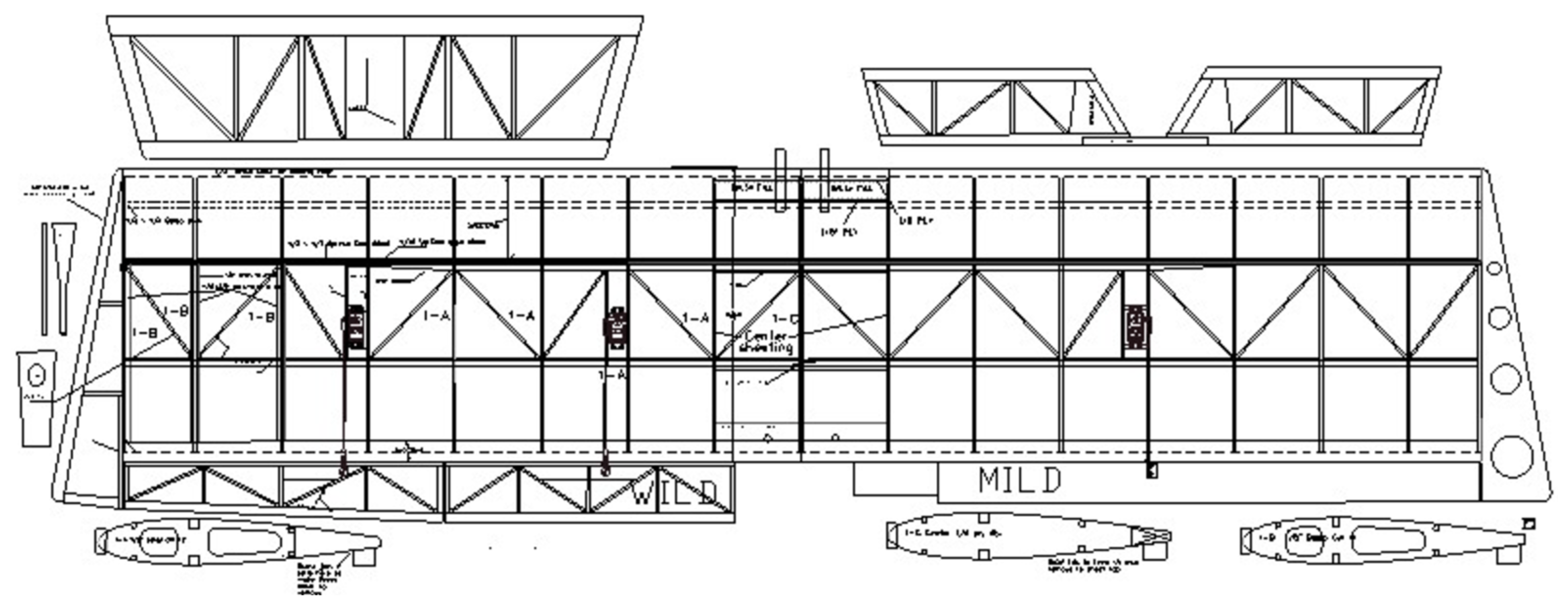
The maximum loading acting on the wing was obtained based on the classical methods of mechanics of materials [46]. Given the cross-section of the wing shown in Figure 4, the section properties were calculated using balsa wood material (Figure 5). The ultimate stress of the wing was estimated using
where M is the internal moment acting on a given section, is the vertical distance to the neutral axis, and is the area moment of inertia. According to the measurements taken from the wing drawing, the approximate ultimate stress for the wing was calculated based on the data from Table 2 using the linear interpolation for the particular size of the thickest stringer and was equal to 9558 psi. For each simulation, the stress was estimated for every stringer.
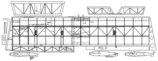
Figure 4.
Ultra Stick 120 Wing Drawing.
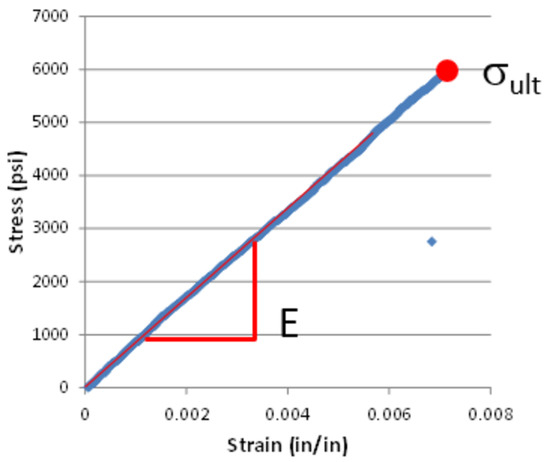
Figure 5.
Balsa Stick Properties.
Table 2.
Tensile strength () and Modulus (E).
7.2. Linear, Parameter-Varying Model
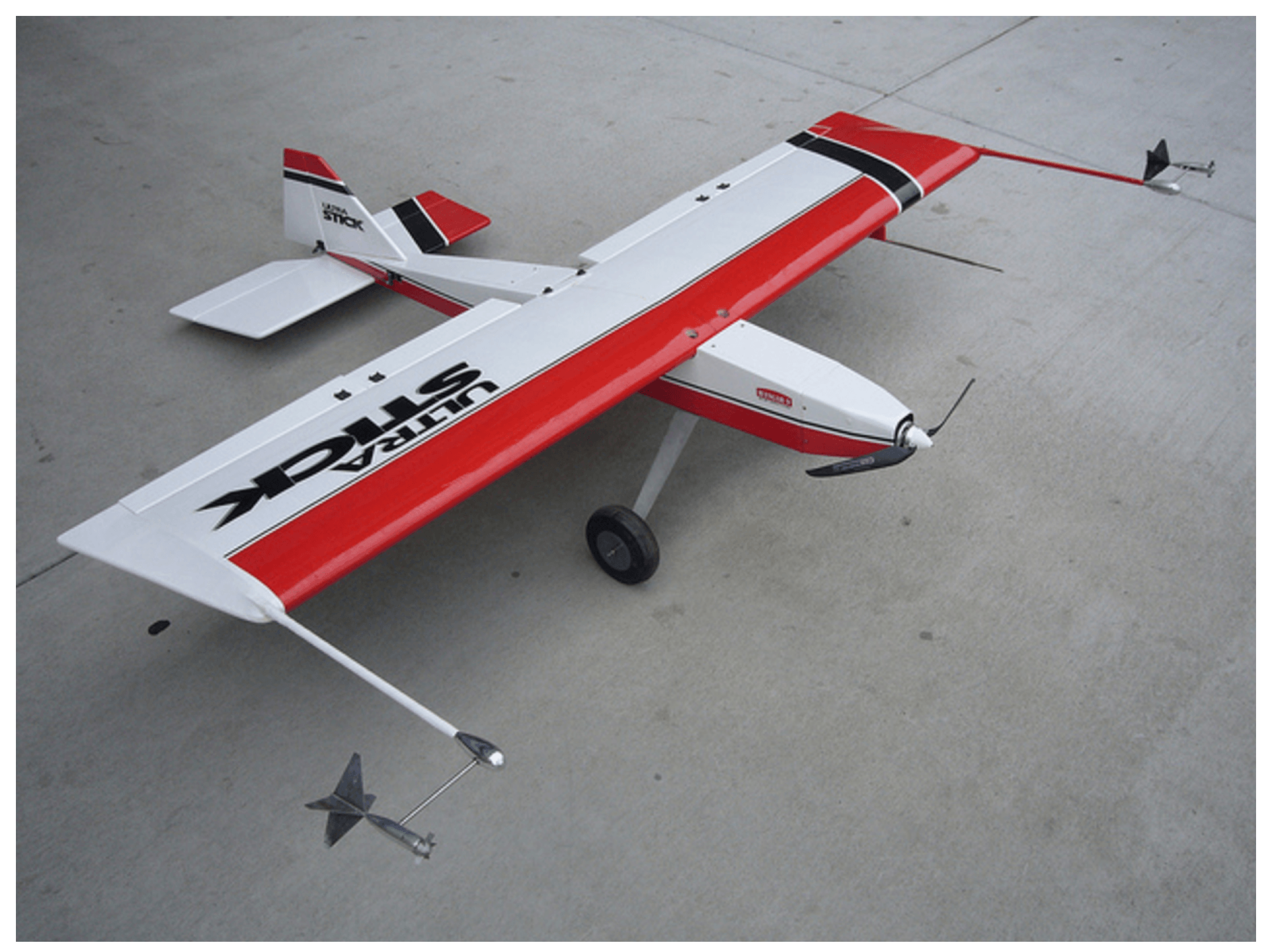
For further comparison of linear vs. nonlinear control designs, here, we employ a linear, parameter-varying (LPV) model based on a small fixed-wing UAV. The UAV selected for numerical simulations is the Ultrastick 120 for which the aerodynamics and flight dynamics have been widely studied [47,48]. Figure 6 shows a picture of the UAV airframe. The LPV model is created by linearizing the nonlinear equations of motion about a set of equilibrium points. Here, the LPV model of the Ultrastick 120 holds a constant pitch/yaw angle and varying airspeed.
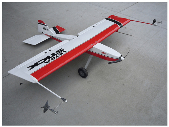
Figure 6.
Ultra Stick 120. Source: UAV Laboratories, University of Minnesota.
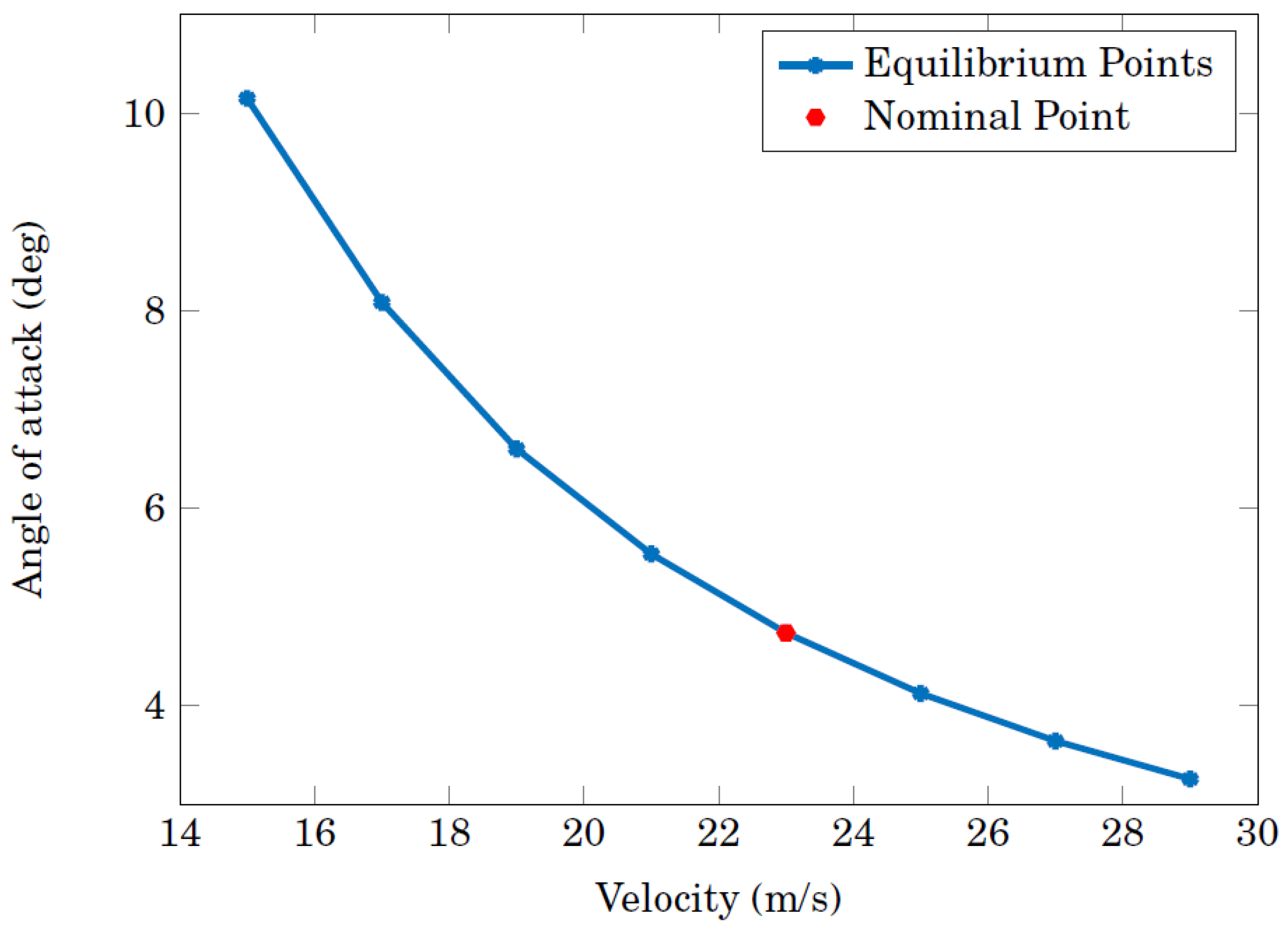
The Ultrastick 120 LPV model is then generated by obtaining a set of equilibrium points holding a constant pitch/yaw angle and varying airspeed between 15 and 29 m/s. These equilibrium points are shown in Figure 7, where airspeed m/s is chosen as the nominal flight condition. Robust nonlinear and linear controllers for such UAVs are designed, with performance analysis presented below.
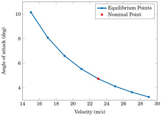
Figure 7.
Varying parameter trajectory: the set of equilibrium points for LPV model.
7.3. Highly Turbulent Case and Take-Off/Landing Cases
The velocity fields are extracted from the LES simulation of the wake vortex in the ground vicinity for two cases: highly turbulent and take-off/landing case. The corresponding vorticity fields are shown in Figure 8. The red dashed line displays the path along which the follower aircraft was swept through the wake vortex behind the follower aircraft (Figure 2). Figure 9, Figure 10, Figure 11, Figure 12, Figure 13 and Figure 14 show the states’ deviations due to wake–vortex–aircraft interaction for a number of points behind the generator aircraft.

Figure 8.
(a) Highly turbulent case. = 600 m/s, t = 132 s, h = 54.5 m (b) The interaction with the secondary vortices during take-off/landing. = 300 m/s, t = 60 s, h = 37 m.
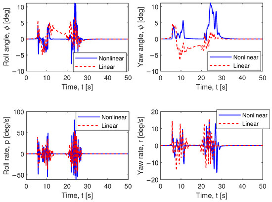
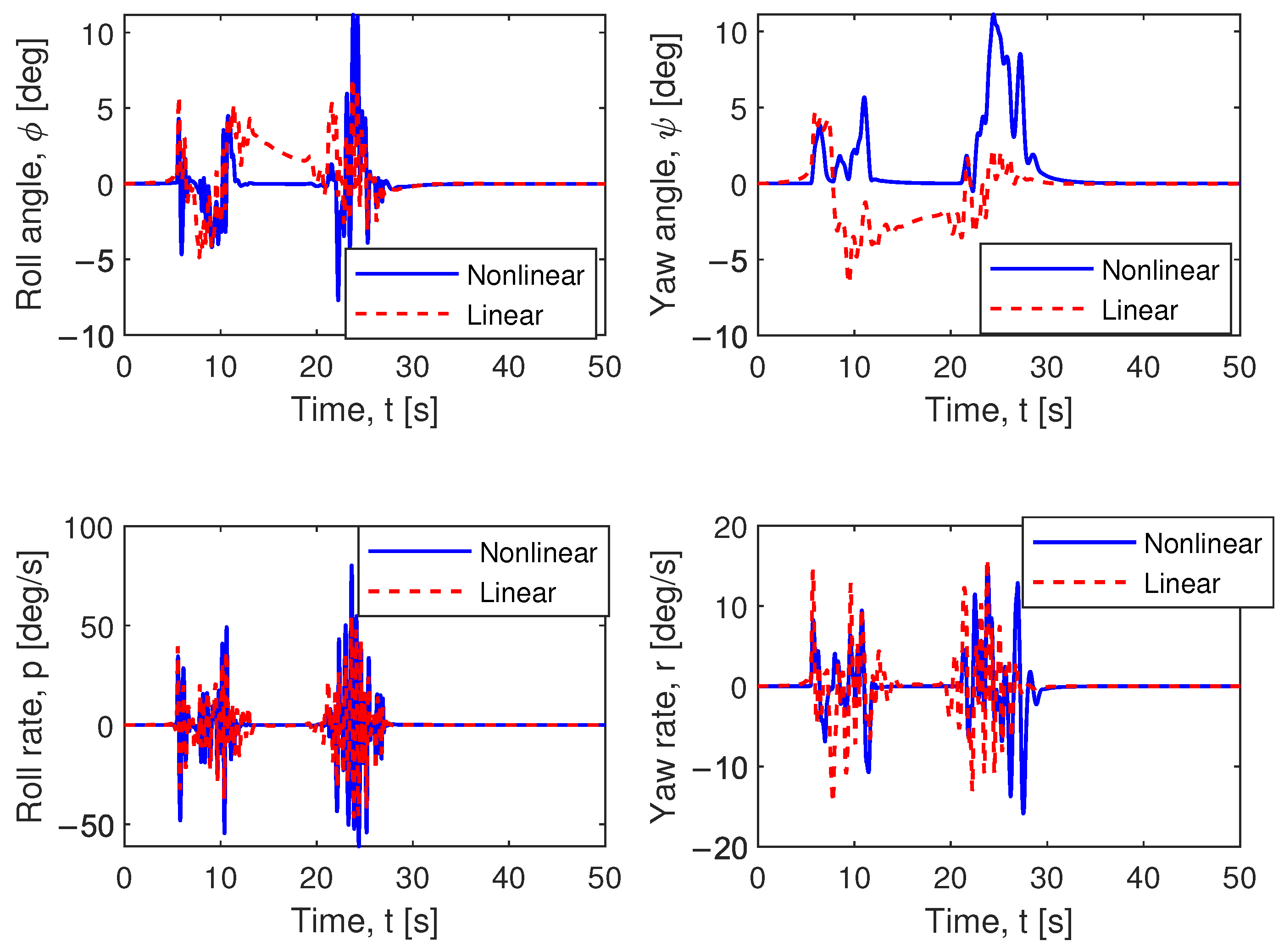
Figure 9.
States deviations for nominal trim point in a highly turbulent case. Nonlinear controller vs. linear controller.

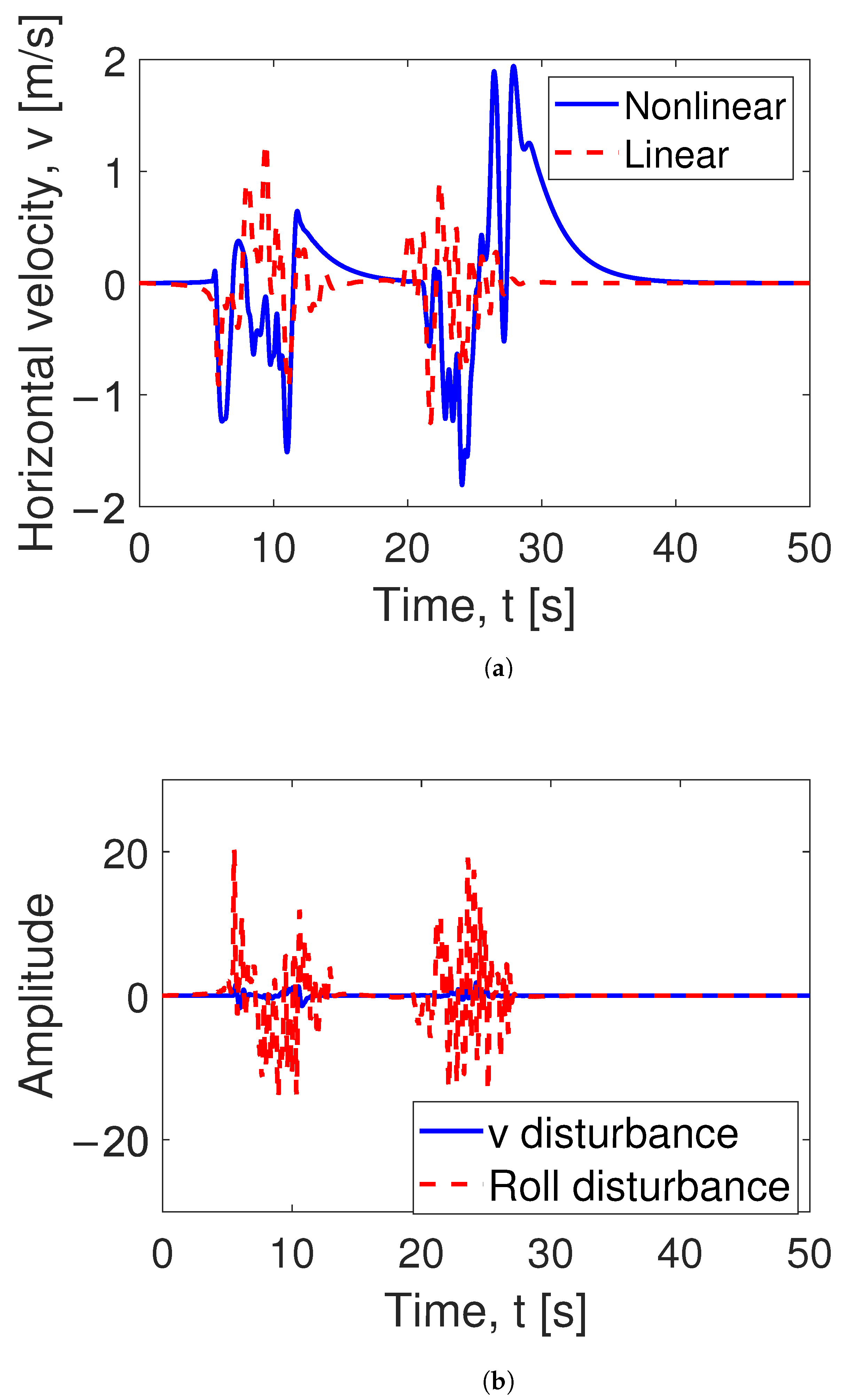
Figure 10.
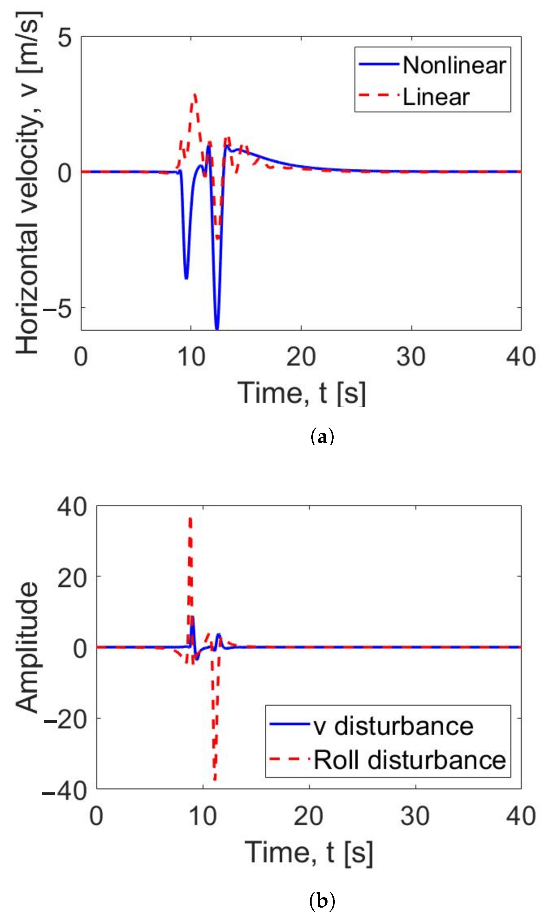
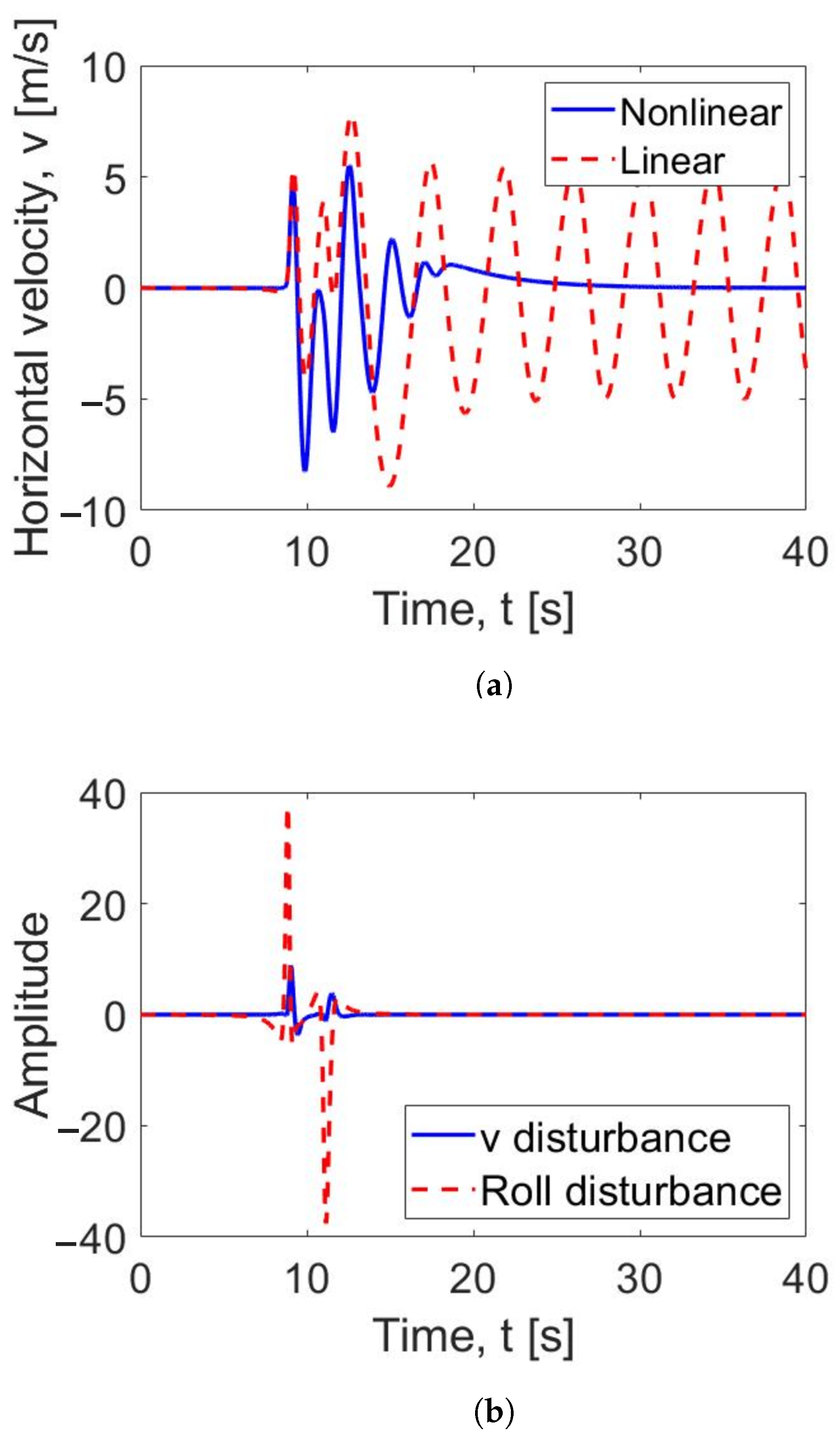
Highly turbulent case. (a) Horizontal velocity and (b) Disturbance. Nonlinear controller vs. linear controller.

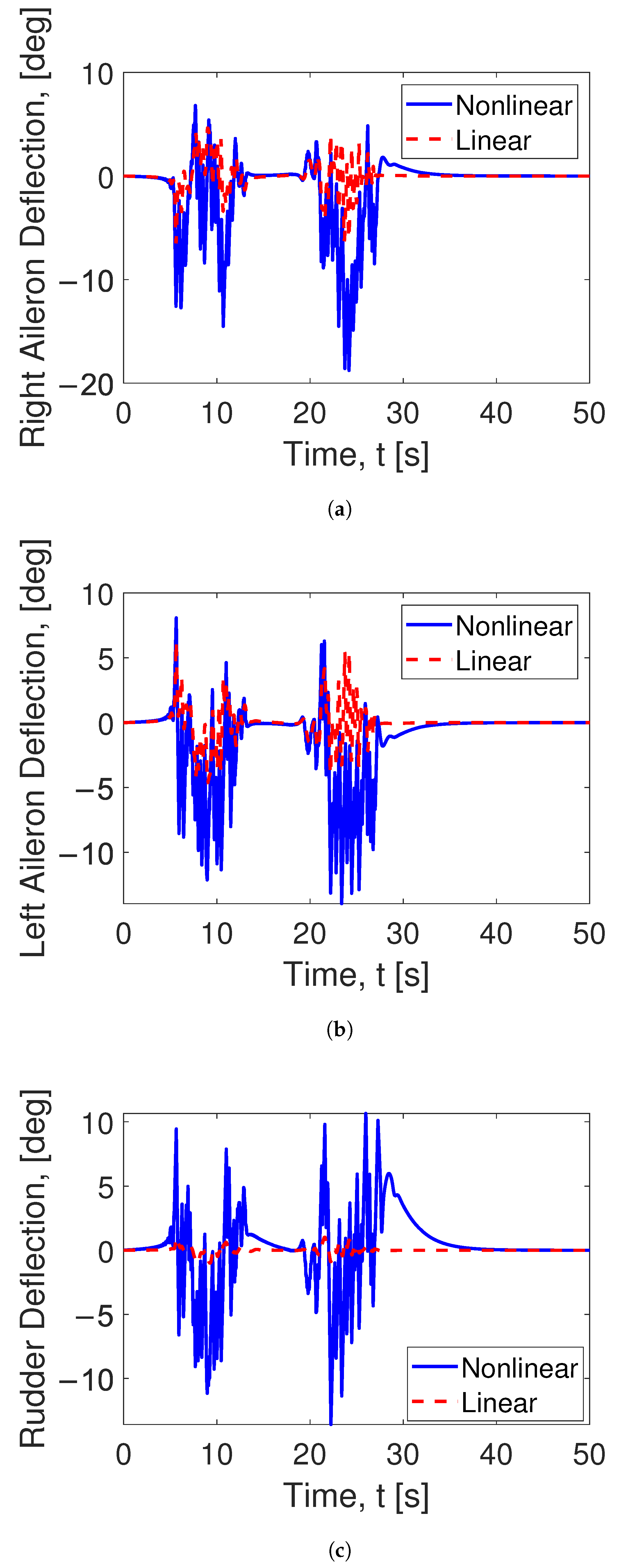
Figure 11.
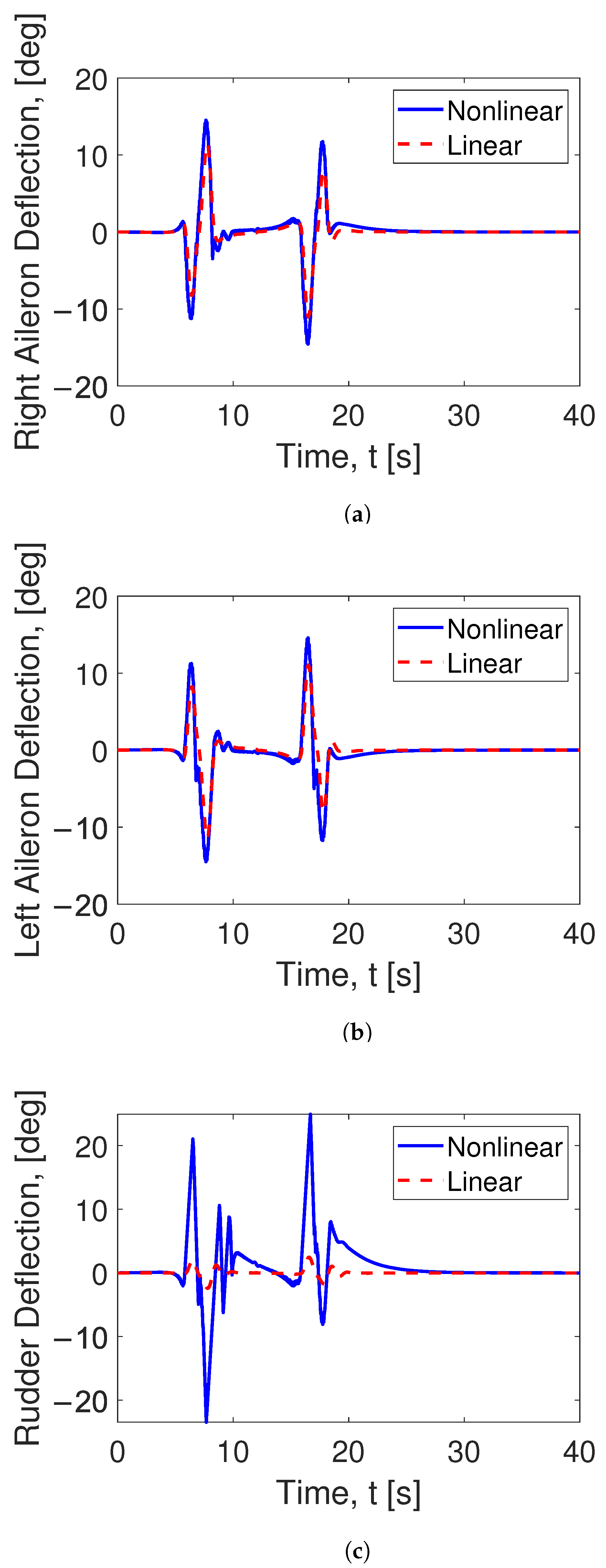
Highly turbulent case. Deflection surfaces deviations for (a) left aileron, (b) right aileron, and (c) rudder. Nonlinear controller vs. linear controller.
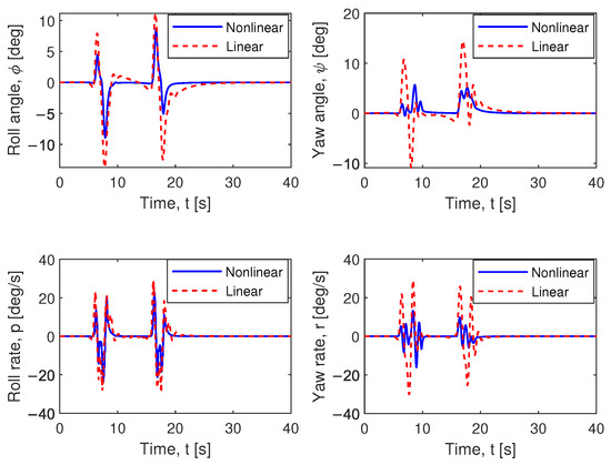
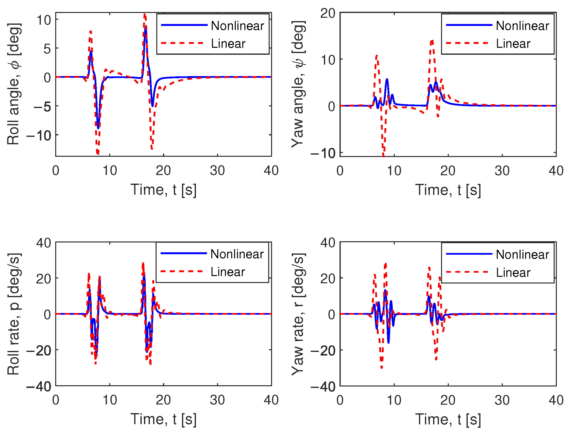
Figure 12.
Take-off/landing case. States deviations for the nominal trim point. Nonlinear controller vs. linear controller.
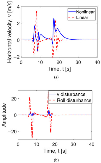
Figure 13.
Take-off/Landing case. (a) Horizontal velocity and (b) Disturbance. Nonlinear controller vs. linear controller.

Figure 14.
Take-off/landing case. Deflection surfaces’ deviations for (a) left aileron, (b) right aileron, and (c) rudder. Nonlinear controller vs. linear controller.
The highly turbulent case reflects the turbulent nature of the wake vortex in a fully developed stage after the roll-up is completed, and the highly turbulent flow in the vicinity of the vortex pair is formed. The parameters of the generator aircraft and flight regime determine the following characteristics of the wake vortex:
- Circulation = 600 m/s
- Vortex core radius = 1.8 m
- Separation distance 30 m
- Current time t = 132 s
The secondary vortices are being destroyed due to the interaction with the primary vortices. The destruction is accompanied by the generation of the turbulence with the opposite vorticity, which triggers the breaking up of the vortex pair and the formation of the smaller vortices. A similar process takes place when the vortex pair interacts with the turbulent atmosphere. The larger the turbulence intensity, the more pronounced the decay is. This case demonstrates the behavior and control of the aircraft interacting with highly turbulent upstream wake vorticity.
Figure 9 and Figure 10 demonstrate the response of the aircraft to the disturbance created by the highly turbulent velocity fields at m from the ground surface and expressed in terms of roll rate disturbance and horizontal velocity disturbance. Roll rate p and yaw rate reactions are similar for both controllers in terms of amplitude and convergence rate. The horizontal velocity v oscillations tend to be bigger for the nonlinear controller. The rudder and ailerons’ deflections (Figure 11) are also bigger in the case of the nonlinear controller. In general, the highly turbulent case is characterized by sharp peaks in each state, which correspond to intense oscillations in the velocity field and the resulting forces and moments acting on the aircraft.
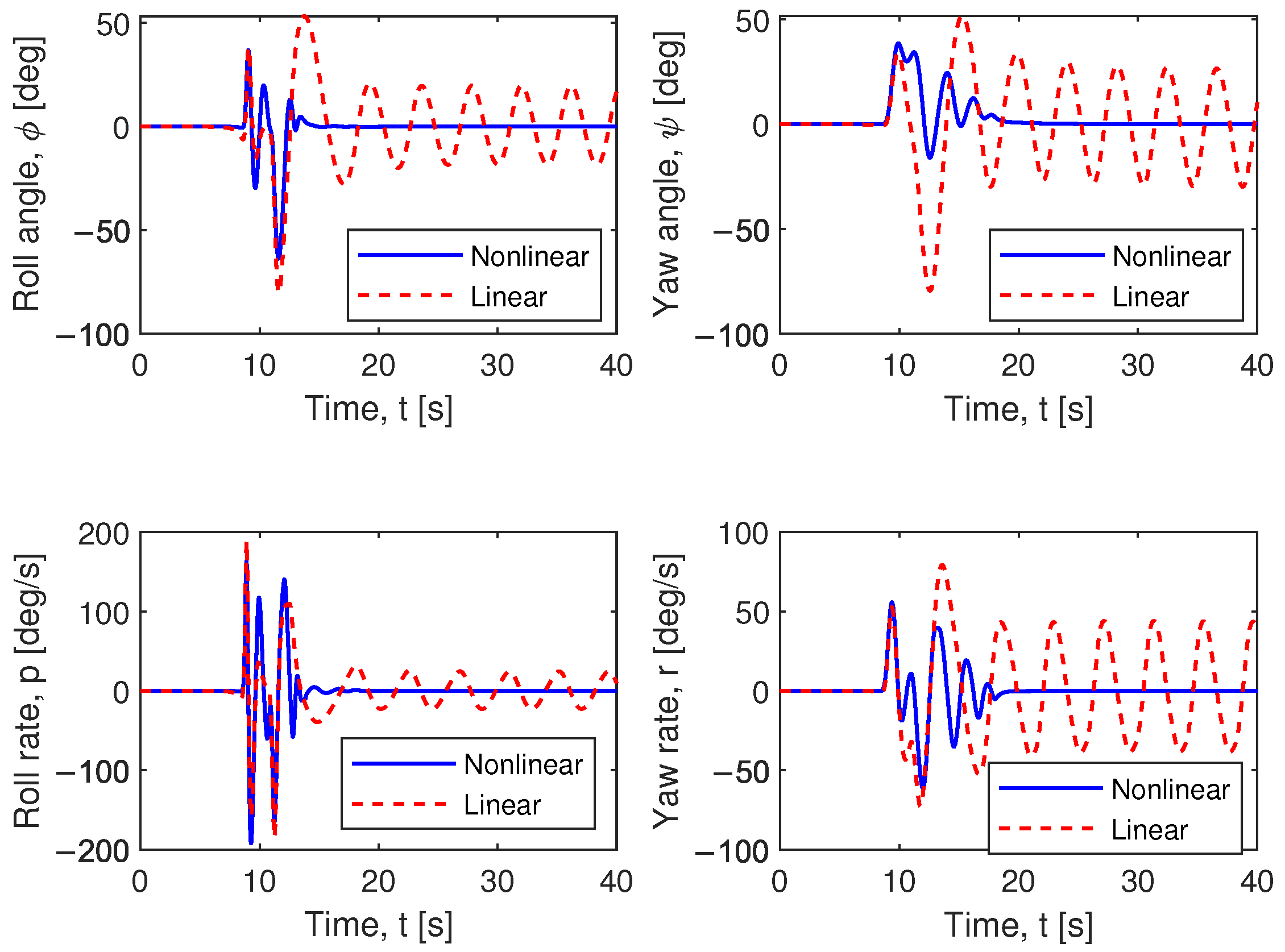
The take-off/landing case is shown in Figure 8b and is characterized by fully formed secondary vortices revolving over the primary ones. This case is different from a highly turbulent one by vortex strength. The trajectory of the follower airplane crosses both of them at H = 37 m from the ground. In this case, the nonlinear controller outperforms the linear one: the maximum amplitude of the states’ deviation is lower, and the convergence time is shorter (Figure 12 and Figure 13a). However, this advantage is reached at the expense of energy spent on surface deflection (Figure 14). The wake vortex is characterized by:
- Circulation = 300 m/s;
- Vortex core radius = 1.8 m;
- Separation distance 30 m;
- Current time t = 60 s.
The convergence rate for roll angle , yaw angle , and roll rate (Figure 12 and Figure 13a) is higher in the case of the nonlinear controller. The maximum deviation for all the states is higher for the controller, which makes the nonlinear controller more efficient. The aileron deviations shown in Figure 14 are almost the same for both controllers; however, the rudder deflection is bigger in the case of the nonlinear controller, which makes it less energy efficient in this case.
7.4. Interaction with Wake Vortex: Steady Level Flight Phase
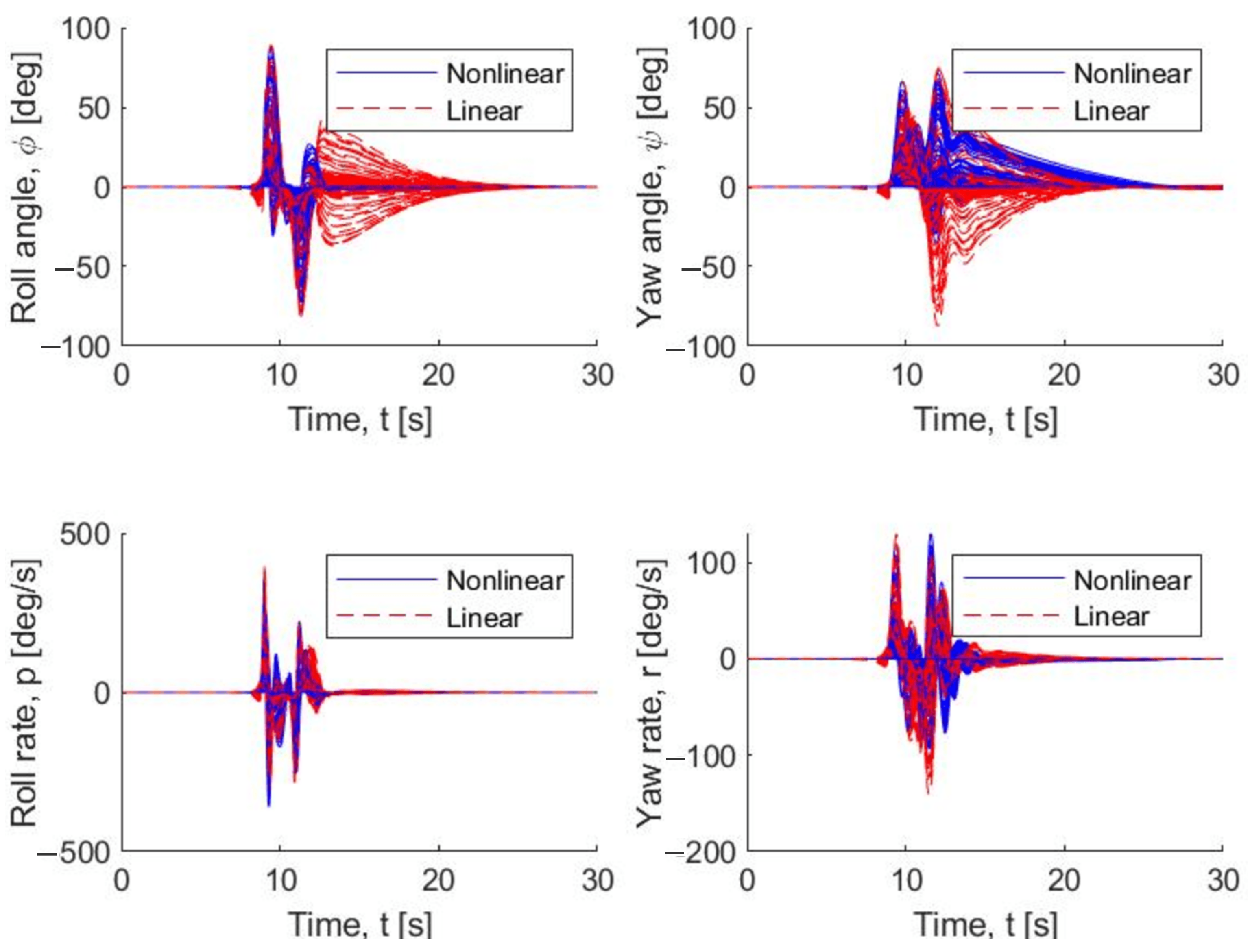
Several sets of Monte Carlo simulations were implemented to model the steady level flight of the aircraft far from the ground in the OGE zone, as indicated in Figure 3, in the presence of the wake vortex. As long as the real wake vortex is affected by the stochastic nature of the turbulent flow generated by the airplane as well as by the interaction with the atmosphere, the exact position of the vortex pair cannot be predicted by the deterministic model. For this reason, the probabilistic approach [31] was used to generate the cone of uncertainty (for wake vortex position and strength), which predicts not the determined position and strength of the wake but the range within which the wake vortex probability to occur is the highest. The first set of simulations was performed for a nominal trim point. The second set corresponds to simulations with parametric uncertainty. Furthermore, structural analysis to estimate the maximum load on the wing was performed. The maximum allowable roll angle deviation less than 90 degrees was set, and the limit of the roll moment was also taken into account.
7.4.1. Nominal Trim Point Simulations
The Monte Carlo simulations for the wake vortex pair were performed based on the real data case from NASA airport experimental measurements [49] wake vortex data set. The approach is based on perturbing the initial wake vortex conditions (, , ) in the deterministic model and generating profiles of the ambient parameters (such as the EDR and potential temperature profiles) using the probability density functions (PDFs). The PDFs are obtained by applying the maximum likelihood estimation method to density histograms corresponding to a particular data set. The vertical profiles are truncated at the heights of the vortex generation and the mean values are calculated from the zero height to that value. A total of 400 perturbations for vertical profiles were generated using PDFs and used as input parameters along with other parametric perturbations. More details of the method can be found in Ref. [34]. The characteristics of the wake generator aircraft (B-722) are:
- Circulation = 262 m/s;
- Span b = 32.9 m;
- Velocity V = 77.8 m/s.
The distance to the generator’s aircraft path line as well as 400 wake vortex realizations were used as an input to the linear and nonlinear control system. The vertical position of the follower aircraft was fixed at z = 175 m. The separation distance between the vortices in the vortex pair, the generator aircraft’s weight, and the vertical distance to the generator aircraft’s flight path are the input parameters for the controllers’ Monte Carlo simulations. Figure 15 shows the nondimensionalized circulation and vertical coordinate of the vortex pair obtained in the first set of simulations, which forms the cone of uncertainty in the real wake vortex evolution. The response of the follower aircraft at the distances of 5.46 nm, 4.16 nm, and 2.34 nm, which correspond to , , and , is considered.
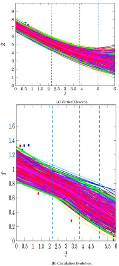
Figure 15.
Wake vortex evolution results based on 400 Monte Carlo simulations. The simulation is performed for (Blue dashed line).
Figure 15 demonstrates the cone of the uncertainty of the wake vortex in terms of vertical coordinate and its strength. Blue dashed lines show the cut that corresponds to the moment of time considered. The plots of the states for each Monte Carlo simulation () are shown in Figure 16. The average Root Mean Square Error (RMSE) and Average Maximum Deviations (AMD) of deflections surfaces metrics are chosen to demonstrate the performance of the controller. The values of the average RMSE and AMD for each state are summarized in Table 3, Table 4 and Table 5. The RMSE for all the states shows that the nonlinear controller is more effective than the linear one in terms of states’ deviations. However, the nonlinear controller uses the rudder more actively and thus expends more energy for control. Furthermore, from the comparison of the RMSE values, one can see that the nonlinear controller works better than the linear one.

Figure 16.
States deviations for a nominal trim point from the MC simulations. Nonlinear controller vs. linear controller.
Table 3.
Average states’ RMSE and Maximum Deviations of Deflection Surfaces over 400 Monte Carlo simulations .
Table 4.
Average states’ RMSE and Maximum Deviations of Deflection Surfaces over 400 Monte Carlo simulations .
Table 5.
Average states’ RMSE and Maximum Deviations of Deflection Surfaces over 400 Monte Carlo simulations .
7.4.2. Simulations with Parametric Uncertainty
The advantage of the nonlinear robust controller is the ability to suppress the disturbance at different flight conditions and aircraft parameter’s deviations. The LPV simulation is performed for several trim points (equilibrium points), which corresponds to the change of parameters of the aircraft and the flight conditions. At the same time, the linear and nonlinear controllers are designed for the nominal trim point. The results are presented in Table 6. The states’ average RMSE and AMD are summarized for , equilibrium point , which corresponds to 27 m/s flight with 3.5 deg angle of attack (Figure 7). It is clear that the nonlinear controller outperforms the linear one. However, this advantage is due to the use of a higher amount of energy spent on the rudder deflection.
Table 6.
Average states’ RMSE and Maximum Deviations of Deflection Surfaces over 400 Monte Carlo simulations. Equilibrium point .
7.4.3. Nonlinear Robust Controller vs. PID Controller
This subsection demonstrates the performance comparison between the nonlinear robust controller and the proportional–integral–derivative controller (PID) in the presence of parametric variations. We model these conditions by choosing different equilibrium (trim) points (Figure 7), as was conducted in the previous section. Both controllers are tuned based on the nominal trim point conditions. In order to compare the performance of two controllers, the Ultrastick 120 is set to follow the B-733 aircraft at the distance where the maximum circulation of the wake is of . The parameters of generator aircraft are:
- Circulation = 230 m/s;
- Span b = 28.9 m;
- Velocity V = 65.7 m/s.
Figure 17 and Figure 18 show the performance of the PID controller vs. the robust nonlinear controller for the nominal trim point. In this case, both controllers show the ability to suppress the disturbance. However, at trim point , the PID controller is not able to compensate for the disturbance, as shown in Figure 19 and Figure 20. Indeed, the nonlinear robust controller’s performance is at the same level as it is at the nominal trim point. This demonstrates the effectiveness of the robust nonlinear control law in the presence of the disturbance.
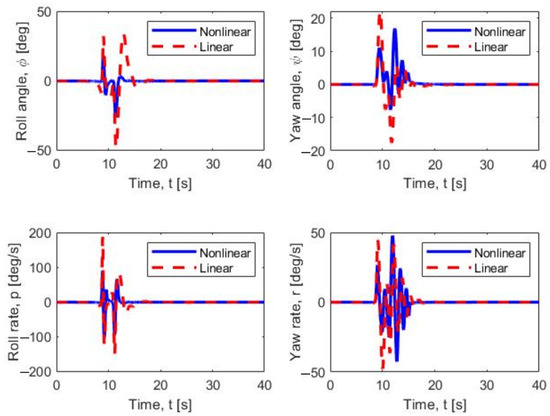
Figure 17.
Steady level flight case. State deviations for a nominal trim point. Nonlinear controller vs. linear PID controller.
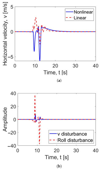
Figure 18.
Steady level flight case. (a) Horizontal velocity and (b) Disturbance. Nominal trim point. Nonlinear controller vs. linear PID controller.
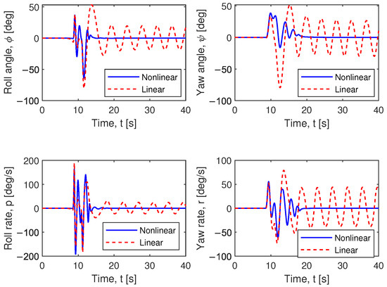
Figure 19.
Steady level flight case. State deviations for trim point #1. Nonlinear controller vs. linear PID controller.
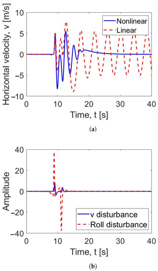
Figure 20.
Steady level flight case. (a) Horizontal velocity and (b) Disturbance. Trim point #1. Nonlinear controller vs. linear PID controller.
8. Conclusions
A robust nonlinear control method is developed and is demonstrated to achieve roll/yaw regulation in the presence of unmodeled external disturbances (i.e., wake vortices and wind gusts) and system nonlinearities. The results of numerical simulations were provided to demonstrate the performance of the proposed nonlinear control law. For comparison, the same control objective was simulated using a linear control law as well as a PID controller. It was shown that the nonlinear control method compensates for the disturbances similarly or more effectively than the linear controller. The PID controller is not capable of rejecting the disturbances in the presence of system nonlinearities. The results showed that the nonlinear control design outperformed the linear control method for the simulated trajectory regulation objective under the tested levels of uncertainty.
The performance of the nonlinear controller was successfully tested in the presence of the wake vortex disturbance in the vicinity of the ground as well as far from the ground, which corresponds to take-off/landing and steady level flight conditions. The interaction of wake vortex-induced turbulence field and aircraft was modeled using high-fidelity Large Eddy Simulations (LES) simulations, which reflect real flight conditions in the terminal zones. The Monte Carlo simulations for the out-of-ground interaction were performed based on the data from the NASA experimental measurements. Using this data, the cone of uncertainty for the wake-vortex evolution was modeled and employed in the simulation. The performance of the robust nonlinear controller and linear controller were compared for both in-ground and out-of-ground zones. The nonlinear controller outperformed the linear one in terms of average Root Mean Square Error (RMSE) and Average Maximum Deviation (AMD).
The results demonstrate the capability of the proposed nonlinear controller to asymptotically reject wake vortex disturbance in the presence of a high degree of uncertainty and nonlinearity in the UAV operating conditions. Moreover, the nonlinear controller is designed with a computationally efficient structure, which is motivated by UAV applications where onboard computational resources are limited.
As a future step, the authors are planning to test the performance of proposed controller on the Ultrastick-120 model in a wind tunnel for the set of wake vortex strengths.
Author Contributions
Formal analysis, P.K., V.G., and W.M.; investigation, P.K.; supervision, V.G., W.M., and C.M.; validation, P.K. and W.M.; writing—original draft, P.K.; writing—review and editing, V.G. and W.M. All authors have read and agree to the published version of the manuscript.
Funding
This research received no external funding.
Conflicts of Interest
The authors declare no conflict of interest.
Abbreviations
The following abbreviations are used in this manuscript:
| UAV | unmanned aerial vehicle |
| UAS | unmanned aerial systems |
| NAS | national airspace system |
| FAA | Federal Aviation Administration |
| MIMO | multi-input multi-output |
| LES | large eddy simulations |
| LPV | linear parameter-varying model |
| PID | proportional–integral–derivative |
| EDR | eddy dissipation rate |
| WVSS | wake vortex safety system |
| RMSE | root mean square error |
| AMD | average maximum deviation |
| probability density function |
Nomenclature
| x | system states |
| u | system inputs |
| y | system outputs |
| f | unknown nonlinear disturbance |
| A | system matrix |
| B | input matrix |
| C | output matrix |
| D | feedthrough matrix |
| t | time, s |
| parametric uncertainty | |
| aileron deflection, | |
| rudder deflection, | |
| v | lateral velocity, |
| p | roll rate, |
| r | yaw rate, |
| roll angle, | |
| left aileron deflection, | |
| right aileron deflection, | |
| p | roll rate, |
| r | yaw rate, |
| roll angle, | |
| left aileron deflection, | |
| right aileron deflection, | |
| rudder deflection, | |
| roll angle, | |
| yaw angle, | |
| auxiliary regulation error | |
| and | auxiliary regulation errors for roll and yaw |
| d | actuation disturbances |
| w | wind gust disturbances |
| uncertainty model weight | |
| actuation disturbance model weight | |
| gain attenuation | |
| controller system gain | |
| and | control gains |
| ultimate stress, | |
| M | internal moment, |
| vertical distance to the neutral axis, | |
| area moment of inertia, | |
| E | tensile modulus, |
| tensile strength, | |
| tangential velocity, | |
| vortex strength, | |
| distance from the vortex center, m | |
| P | proportional gain |
| I | integral gain |
| D | derivative gain |
References
- Borener, S.; Trajkov, S.; Balakrishna, P. Design and development of an integrated safety assessment model for nextgen. In Proceedings of the International Annual Conference of the American Society for Engineering Management, San Antonio, TX, USA, 10–13 June 2012. [Google Scholar]
- Rysdyk, R. Unmanned aerial vehicle path following for target observation in wind. J. Guid. Control. Dyn. 2006, 29, 1092–1100. [Google Scholar] [CrossRef]
- Liu, C.; Chen, W.H. Disturbance rejection flight control for small fixed-wing unmanned aerial vehicles. J. Guid. Control. Dyn. 2016, 2810–2819. [Google Scholar] [CrossRef] [Green Version]
- Okamoto, K.; Tsuchiya, T. Optimal aircraft control in stochastic severe weather conditions. J. Guid. Control. Dyn. 2015, 39, 77–85. [Google Scholar] [CrossRef]
- Zhang, Y.; Wang, S.H.; Chang, B.; Wu, W.H. Adaptive constrained backstepping controller with prescribed performance methodology for carrier-based UAV. Aerosp. Sci. Technol. 2019, 92, 55–65. [Google Scholar] [CrossRef]
- Dydek, Z.T.; Annaswamy, A.M.; Lavretsky, E. Adaptive control of quadrotor UAVs: A design trade study with flight evaluations. IEEE Trans. Control Syst. Technol. 2013, 21, 1400–1406. [Google Scholar] [CrossRef]
- Bhandari, S.; Patel, N. Nonlinear adaptive control of a fixed-wing UAV using multilayer perceptrons. In Proceedings of the AIAA Guidance, Navigation, and Control Conference, Grapevine, TX, USA, 9–13 January 2017; p. 1524. [Google Scholar] [CrossRef]
- Razmi, H.; Afshinfar, S. Neural network-based adaptive sliding mode control design for position and attitude control of a quadrotor UAV. Aerosp. Sci. Technol. 2019, 91, 12–27. [Google Scholar] [CrossRef]
- Noble, D.; Bhandari, S. Neural network based nonlinear model reference adaptive controller for an unmanned aerial vehicle. In Proceedings of the 2017 International Conference on Unmanned Aircraft Systems (ICUAS), Miami, FL, USA, 13–16 June 2017; pp. 94–103. [Google Scholar] [CrossRef]
- Smeur, E.J.; Chu, Q.; de Croon, G.C. Adaptive incremental nonlinear dynamic inversion for attitude control of micro air vehicles. J. Guid. Control. Dyn. 2015, 38, 450–461. [Google Scholar] [CrossRef] [Green Version]
- Mullen, J.; Bailey, S.C.; Hoagg, J.B. Filtered dynamic inversion for altitude control of fixed-wing unmanned air vehicles. Aerosp. Sci. Technol. 2016, 54, 241–252. [Google Scholar] [CrossRef] [Green Version]
- González-Arribas, D.; Soler, M.; Sanjurjo-Rivo, M.; Kamgarpour, M.; Simarro, J. Robust aircraft trajectory planning under uncertain convective environments with optimal control and rapidly developing thunderstorms. Aerosp. Sci. Technol. 2019, 89, 445–459. [Google Scholar] [CrossRef] [Green Version]
- Matsuno, Y.; Tsuchiya, T.; Wei, J.; Hwang, I.; Matayoshi, N. Stochastic optimal control for aircraft conflict resolution under wind uncertainty. Aerosp. Sci. Technol. 2015, 43, 77–88. [Google Scholar] [CrossRef]
- Yit, K.K.; Rajendran, P.; Wee, L.K. Proportional-derivative linear quadratic regulator controller design for improved longitudinal motion control of unmanned aerial vehicles. Int. J. Micro Air Veh. 2016, 8, 41–50. [Google Scholar] [CrossRef] [Green Version]
- Sun, Y.; Xian, N.; Duan, H. Linear-quadratic regulator controller design for quadrotor based on pigeon-inspired optimization. Aircr. Eng. Aerosp. Technol. 2016, 88, 761–770. [Google Scholar] [CrossRef]
- Huang, J.; Lin, C.F. Numerical approach to computing nonlinear H-infinity control laws. J. Guid. Control. Dyn. 1995, 18, 989–994. [Google Scholar] [CrossRef]
- Jafar, A.; Fasih-UR-Rehman, S.; Fazal-UR-Rehman, S.; Ahmed, N. H Infinity Controller for Unmanned Aerial Vehicle Against Atmospheric Turbulence. Am. Eurasian J. Sci. Res. 2016, 11, 305–312. [Google Scholar] [CrossRef]
- Hegde, N.; George, V.; Nayak, G.C. Design of H-Infinity Loop Shaping Controller for an Unmanned Aerial Vehicle. J. Adv. Res. Dyn. Control Syst. 2018, 10, 65–74. [Google Scholar]
- Pedroza, N.R.; MacKunis, W.; Golubev, V.V. Robust Nonlinear Regulation of Limit Cycle Oscillations in UAVs Using Synthetic Jet Actuators. Robotics 2014, 3, 330–348. [Google Scholar] [CrossRef] [Green Version]
- MacKunis, W.; Subramanian, S.; Mehta, S.; Ton, C.; Curtis, J.W.; Reyhanoglu, M. Robust nonlinear aircraft tracking control using synthetic jet actuators. In Proceedings of the 52nd IEEE Conference on Decision and Control, Firenze, Italy, 10–13 December 2013; pp. 220–225. [Google Scholar] [CrossRef]
- Drakunov, S.V. Sliding-mode observers based on equivalent control method. In Proceedings of the 31st IEEE Conference on Decision and Control, Tucson, AZ, USA, 16–18 December 1992; pp. 2368–2369. [Google Scholar] [CrossRef] [Green Version]
- Vu, M.T.; Le, T.H.; Thanh, H.L.N.N.; Huynh, T.T.; Van, M.; Hoang, Q.D.; Do, T.D. Robust position control of an over-actuated underwater vehicle under model uncertainties and ocean current effects using dynamic sliding mode surface and optimal allocation control. Sensors 2021, 21, 747. [Google Scholar] [CrossRef] [PubMed]
- Vu, M.T.; Le Thanh, H.N.N.; Huynh, T.T.; Thang, Q.; Duc, T.; Hoang, Q.D.; Le, T.H. Station-keeping control of a hovering over-actuated autonomous underwater vehicle under ocean current effects and model uncertainties in horizontal plane. IEEE Access 2021, 9, 6855–6867. [Google Scholar] [CrossRef]
- Xu, H.; Hinostroza, M.A.; Guedes Soares, C. Modified Vector Field Path-Following Control System for an Underactuated Autonomous Surface Ship Modelin the Presence of Static Obstacles. J. Mar. Sci. Eng. 2021, 9, 652. [Google Scholar] [CrossRef]
- Labbadi, M.; Cherkaoui, M. Robust adaptive backstepping fast terminal sliding mode controller for uncertain quadrotor UAV. Aerosp. Sci. Technol. 2019, 93, 105306. [Google Scholar] [CrossRef]
- Ha, L.N.N.T.; Hong, S.K. Robust dynamic sliding mode control-based PID–super twisting algorithm and disturbance observer for second-order nonlinear systems: Application to UAVs. Electronics 2019, 8, 760. [Google Scholar] [CrossRef] [Green Version]
- Thanh, H.L.N.N.; Vu, M.T.; Mung, N.X.; Nguyen, N.P.; Phuong, N.T. Perturbation observer-based robust control using a multiple sliding surfaces for nonlinear systems with influences of matched and unmatched uncertainties. Mathematics 2020, 8, 1371. [Google Scholar] [CrossRef]
- Pan, H.; Zhang, G.; Ouyang, H.; Mei, L. A novel global fast terminal sliding mode control scheme for second-order systems. IEEE Access 2020, 8, 22758–22769. [Google Scholar] [CrossRef]
- Yu, Z.; Qu, Y.; Zhang, Y. Safe control of trailing UAV in close formation flight against actuator fault and wake vortex effect. Aerosp. Sci. Technol. 2018, 77, 189–205. [Google Scholar] [CrossRef]
- Kazarin, P.S.; MacKunis, W.; Moreno, C.; Golubev, V.V. Robust Nonlinear Tracking Control for Unmanned Aircraft with Synthetic Jet Actuators. In Proceedings of the AIAA Atmospheric Flight Mechanics Conference, Denver, CO, USA, 5–9 June 2017; p. 3730. [Google Scholar]
- Kazarin, P.S.; Golubev, V.V. Comparison of Probabilistic Approaches for Predicting the Cone of Uncertainty in Aircraft Wake Vortex Evolution. In Proceedings of the 9th AIAA Atmospheric and Space Environments Conference, Denver, CO, USA, 5–9 June 2017; p. 4369. [Google Scholar] [CrossRef]
- Kazarin, P.S.; Golubev, V.V. On Effects of Ground Surface Conditions On Aircraft Wake Vortex Evolution. In Proceedings of the 9th AIAA Atmospheric and Space Environments Conference, Denver, CO, USA, 5–9 June 2017; p. 4368. [Google Scholar] [CrossRef]
- Kazarin, P.; Golubev, V.V. High-Fidelity Simulations of Terminal-Zone Heterogeneous Terrain Effects On Aircraft Wake Vortex Evolution. In Proceedings of the 2018 AIAA Aerospace Sciences Meeting, Kissimmee, FL, USA, 8–12 January 2018; p. 1279. [Google Scholar] [CrossRef]
- Kazarin, P.; Golubev, V.; Provalov, A.; Borener, S.; Hufty, D. A Variable-Fidelity Approach to Wake Safety Analysis in the Context of UAS Integration in the NAS. In Proceedings of the 16th AIAA Aviation Technology, Integration, and Operations Conference, Washington, DC, USA, 13–17 June 2016; p. 3452. [Google Scholar] [CrossRef]
- Lind, R. Linear parameter-varying modeling and control of structural dynamics with aerothermoelastic effects. J. Guid. Control. Dyn. 2002, 25, 733–739. [Google Scholar] [CrossRef] [Green Version]
- Deb, D.; Tao, G.; Burkholder, J.O.; Smith, D.R. An adaptive inverse control scheme for a synthetic jet actuator model. In Proceedings of the 2005, American Control Conference, Portland, OR, USA, 8–10 June 2005; pp. 2646–2651. [Google Scholar] [CrossRef]
- Deb, D.; Tao, G.; Burkholder, J.O.; Smith, D.R. Adaptive compensation control of synthetic jet actuator arrays for airfoil virtual shaping. J. Aircr. 2007, 44, 616–626. [Google Scholar] [CrossRef]
- Deb, D.; Tao, G.; Burkholder, J.O.; Smith, D.R. Adaptive synthetic jet actuator compensation for a nonlinear aircraft model at low angles of attack. IEEE Trans. Control Syst. Technol. 2008, 16, 983–995. [Google Scholar] [CrossRef]
- Tchieu, A.A.; Kutay, A.T.; Muse, J.A.; Calise, A.J.; Leonard, A. Validation of a low-order model for closed-loop flow control enable flight. AIAA Pap. 2008, 3863. [Google Scholar] [CrossRef]
- Singhal, C.; Tao, G.; Burkholder, J.O. Neural network-based compensation of synthetic jet actuator nonlinearities for aircraft flight control. In Proceedings of the AIAA Guidance, Navigation, and Control Conference, Chicago, IL, USA, 10–13 August 2009; Volume 1013, p. 119. [Google Scholar] [CrossRef]
- Mondschein, S.T.; Tao, G.; Burkholder, J.O. Adaptive actuator nonlinearity compensation and disturbance rejection with an aircraft application. In Proceedings of the 2011 American Control Conference, San Francisco, CA, USA, 29 June–1 July 2011; pp. 2951–2956. [Google Scholar] [CrossRef]
- Zhou, K.; Doyle, J.; Glover, K. Robust and Optimal Control; Prentice Hall: Hoboken, NJ, USA, 1995; Chapter 10; pp. 251–253. [Google Scholar]
- Kidambi, K.B.; Ramos-Pedroza, N.; MacKunis, W.; Drakunov, S.V. Robust nonlinear estimation and control of fluid flow velocity fields. In Proceedings of the 2016 IEEE 55th Conference on Decision and Control (CDC), Las Vegas, NV, USA, 12–14 December 2016; pp. 6727–6732. [Google Scholar] [CrossRef]
- Burnham, D.C.; Hallock, J.N. Chicago Monostatic Acoustic Vortex Sensing System. Volume IV. Wake Vortex Decay; Technical Report, DTIC Document; U.S. Department of Transportation: Washington, DC, USA, 1982.
- Kazarin, P. Variable Fidelity Studies in Wake Vortex Evolution, Safety, and Control; Embry-Riddle Aeronautical University: Daytona Beach, FL, USA, 2018. [Google Scholar]
- Anderson, J.D. Aircraft Performance and Design; McGraw-Hill Science/Engineering/Math: New York, NY, USA, 1999; Chapter 8; p. 410. [Google Scholar]
- Freeman, P.M. Reliability Assessment for Low-Cost Unmanned Aerial Vehicles. Ph.D. Thesis, University of Minnesota, Minneapolis, MN, USA, 2014. [Google Scholar]
- Dorobantu, A.; Murch, A.; Mettler, B.; Balas, G. Frequency Domain System Identification for a Small, Low-Cost, Fixed-Wing UAV. In Proceedings of the AIAA Guidance, Navigation, and Control Conference, Portland, OR, USA, 8–11 August 2011; pp. 6–11. [Google Scholar] [CrossRef] [Green Version]
- Gloudemans, T.; Van Lochem, S.; Ras, E.; Malissa, J.; Ahmad, N.N.; Lewis, T.A. A Coupled Probabilistic Wake Vortex and Aircraft Response Prediction Model; NASA TM-2016-219193; NASA: Washington, DC, UAA, 2016.


Publisher’s Note: MDPI stays neutral with regard to jurisdictional claims in published maps and institutional affiliations. |
© 2021 by the authors. Licensee MDPI, Basel, Switzerland. This article is an open access article distributed under the terms and conditions of the Creative Commons Attribution (CC BY) license (https://creativecommons.org/licenses/by/4.0/).