Abstract
Convolutional neural networks (CNN) can achieve accurate image classification, indicating the current best performance of deep learning algorithms. However, the complexity of spectral data limits the performance of many CNN models. Due to the potential redundancy and noise of the spectral data, the standard CNN model is usually unable to perform correct spectral classification. Furthermore, deeper CNN architectures also face some difficulties when other network layers are added, which hinders the network convergence and produces low classification accuracy. To alleviate these problems, we proposed a new CNN architecture specially designed for 2D spectral data. Firstly, we collected the reflectance spectra of five samples using a portable optical fiber spectrometer and converted them into 2D matrix data to adapt to the deep learning algorithms’ feature extraction. Secondly, the number of convolutional layers and pooling layers were adjusted according to the characteristics of the spectral data to enhance the feature extraction ability. Finally, the discard rate selection principle of the dropout layer was determined by visual analysis to improve the classification accuracy. Experimental results demonstrate our CNN system, which has advantages over the traditional AlexNet, Unet, and support vector machine (SVM)-based approaches in many aspects, such as easy implementation, short time, higher accuracy, and strong robustness.
1. Introduction
The emergence of the Internet of Things (IoT) has promoted the rise of edge computing. In IoT applications, data processing, analysis, and storage are increasingly occurring at the edge of the network, close to where users and devices need to access information, which makes edge computing an important development direction.
There were already applications of deep learning in IoT, for example, deep learning predicted household electricity consumption based on data collected by smart meters [1]; and a load balancing scheme based on the deep learning of the IoT was introduced [2]. Through the analysis of a large amount of user data, the network load and processing configuration are measured, and the deep belief network method is adopted to achieve efficient load balancing in the IoT. In [3], an IoT data analysis method based on deep learning algorithms and Apache Spark was proposed. The inference phase was executed on mobile devices, while Apache Spark was deployed in the cloud server to support data training. This two-tier design was very similar to edge computing, which showed that processing tasks can be offloaded from the cloud. In [4], it is proven that due to the limited network performance of data transmission, the centralized cloud computing structure can no longer process and analyze the large amount of data collected from IoT devices. In [5], the authors indicated that edge computing can offload computing tasks from the centralized cloud to the edge near the IoT devices, and the data transmitted during the preprocessing process will be greatly reduced. This operation made edge computing another key technology for IoT services.
The data generated by IoT sensor terminal devices need to use deep learning for real-time analysis or for training deep learning models. However, deep learning [6] inference and training require a lot of computing resources to run quickly. Edge computing is a viable method, as it stores a large number of computing nodes at the terminal location to meet the requirements of high computation and low latency of edge devices. It shows good performance in privacy, bandwidth efficiency, and scalability. Edge computing has been applied to deep learning with different aims: fabric defect detection [7], falling detection in smart cities, street garbage detection and classification [8], multi-task partial computation offloading and network flow scheduling [9], road accidents detection [10], and real-time video optimization [11].
Red, green, and blue (RGB) cameras mainly use red, green, and blue light to classify objects. From the point of view of the spectrum, there are three bands that are only in the visible band. The number of spectral bands we use has 1024, including some near-infrared light bands, which is more helpful for accurate classifications. For instance, the red-edge effect of the infrared band inside can distinguish real leaves from plastic leaves in vegetation detection. Therefore, we believe that increasing the number of spectral channels is more conducive to the application expansion of the system in the future.
The optical fiber spectrometer has been reported for applications in photo-luminescence properties detection [12], the smartphone spectral self-calibration [13], and phosphor thermometry [14]. At present, some imaging spectrometers can obtain spatial images, depth information, and spectral data of objects simultaneously [15]. However, most of the data processed by deep learning algorithms are image data information obtained by these imaging spectrometers. Deep learning algorithms are rarely used to process the reflection spectrum data obtained by the optical fiber spectrometer.
In hyperspectral remote sensing, deep learning algorithms have been widely applied to hyperspectral imaging classification processing tasks. For example, in [16], a spatial-spectral feature extraction framework for robust hyperspectral images classification was proposed to combine a 3D convolutional neural network. Testing overall classification accuracies was 4.23% higher than SVM on Pavia data sets and Pines data sets. In [17], a new recurrent neural network architecture was designed and the testing accuracy was 11.52% higher than that of a long short-term memory network, which is on the HSI data sets Pavia and Salinas. A new recursive neural network structure was designed in [18], and an approach based on a deep belief network was introduced for hyperspectral images classification. Compared with SVM, overall classification accuracies of Salinas, Pines, and Pavia data sets increased by 3.17%. Currently, hyperspectral imagers are mainly used to detect objects [19]. Although the optical fiber spectrometer is easy to carry and collect the spectra of objects, it cannot realize the imaging detection research of objects. However, deep learning algorithms are data-driven and can realize end-to-end feature processing. If we process spectral data by combining deep learning algorithms with fiber optic spectrometers, it can further perform the detection and research of objects.
However, most spectrometers need to be connected to the host computer via USB, which cannot be carried easily. In this work, we designed and manufactured a portable optical fiber spectrometer. After testing the stability of the system, we collected the reflectance spectra of five fruit samples and proposed a depth called the convolutional neural network learning method, which performs spectral classification. The accuracy of this method is 94.78%. We boldly combined the deep learning algorithm and the system to complete the accurate classification of spectral data. Using this portable spectrometer, we use edge computing technology to increase the speed of deep learning while processing spectral data.
We have designed a portable spectrometer with a screen; the system can get rid of the heavy host computer and realize real-time detection of fruit quality.
Our portable spectrometer is shown in Figure 1a. The spectrometer has a 5-inch touch screen, and users can view the visualized sample spectrum information on the spectrometer in real-time. As shown in Figure 1b, the system is equipped with an Ocean Optics-USB2000+ spectrometer (Ocean Optics, Delray Beach, FL, USA), to ensure that the system has a spectral resolution of not less than 5nm. As shown in Figure 1d, the system configuration of our spectrometer is a GOLE1 microcomputer, Ocean Optics USB2000+ spectrometer, and a high-precision packaging fixture. The optical fiber can be connected with the spectrometer through a fine-pitch mechanical thread. The overall structure is treated with electroplating black paint, to effectively avoid external light interference and greatly improve the signal-to-noise ratio of spectral information. When using our spectrometer to detect samples, we connect one end of the optical fiber to the spectrometer through a mechanical thread and hold the other end close to the test sample. The reflected light from the sample surface enters the spectrometer through the optical fiber, and the spectrometer converts the collected optical information into electrical signals and transmits it to the microcomputer through the USB cable. The microcomputer visualizes the signal on the screen. Users can view, store, and transmit spectral information through the system’s touch screen, innovating the functions of traditional spectrometers that need to be operated by the keyboard and mouse of the host computer.
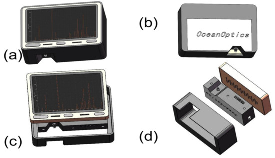
Figure 1.
(a) The GOLE1 mini-computer used in the experiment. (b) The Ocean Optics USB2000+ spectrometer that was used in the experiment. (c) Front view of the assembly of the mini-computer and the spectrometer; (d) Integration of the spectrometer and the mini-computer through a self-designed housing.
To ensure the accuracy of the system data acquisition and to demonstrate the system’s ability to detect various data, the team tested the stability of the entire hyperspectral imaging system. First, we adjust the imaging to the same state as the data acquisition, then we collect 10 sets of solar light spectral data by the spectrograph at 10 s intervals; then, we adjust the display of the system to red, green, and blue colors in turn, and repeat the above steps to obtain the corresponding data. Finally, we input 40 groups of data collected by the above methods into Matlab and then use two different processing methods to demonstrate the stability of the whole hyperspectral imaging system.
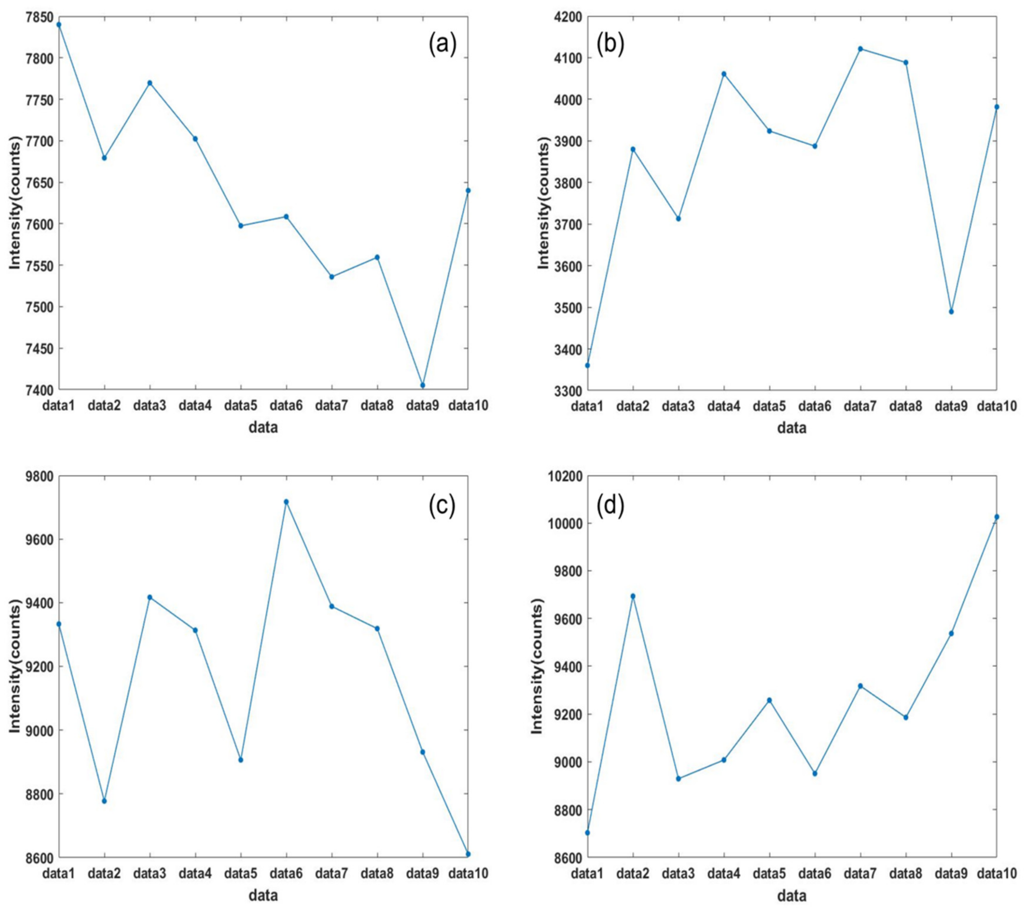
The first method is to extract one data point of the same wavelength from all 10 groups of data of the same kind, and arrange the data points in order and draw them into the pictures as shown below.
As shown in Figure 2, we can see clearly that the intensity fluctuation of the same 10 groups of data at the same wavelength is very small. This shows that the error of data acquisition of the same object is very small in a short time, which proves that the system has high accuracy.
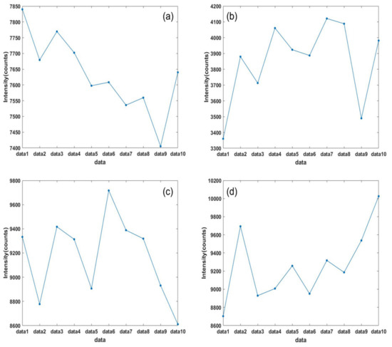
Figure 2.
(a) Point data of the same wavelength of 10 sets of sunlight spectrum data collected every 10 s. (b) Point data of the same wavelength of 10 sets of screen green light spectrum data collected every 10 s. (c) Point data of the same wavelength of 10 sets of screen blue light spectrum data collected every 10 s. (d) Point data of the same wavelength of 10 sets of screen red light spectrum data collected every 10 s.
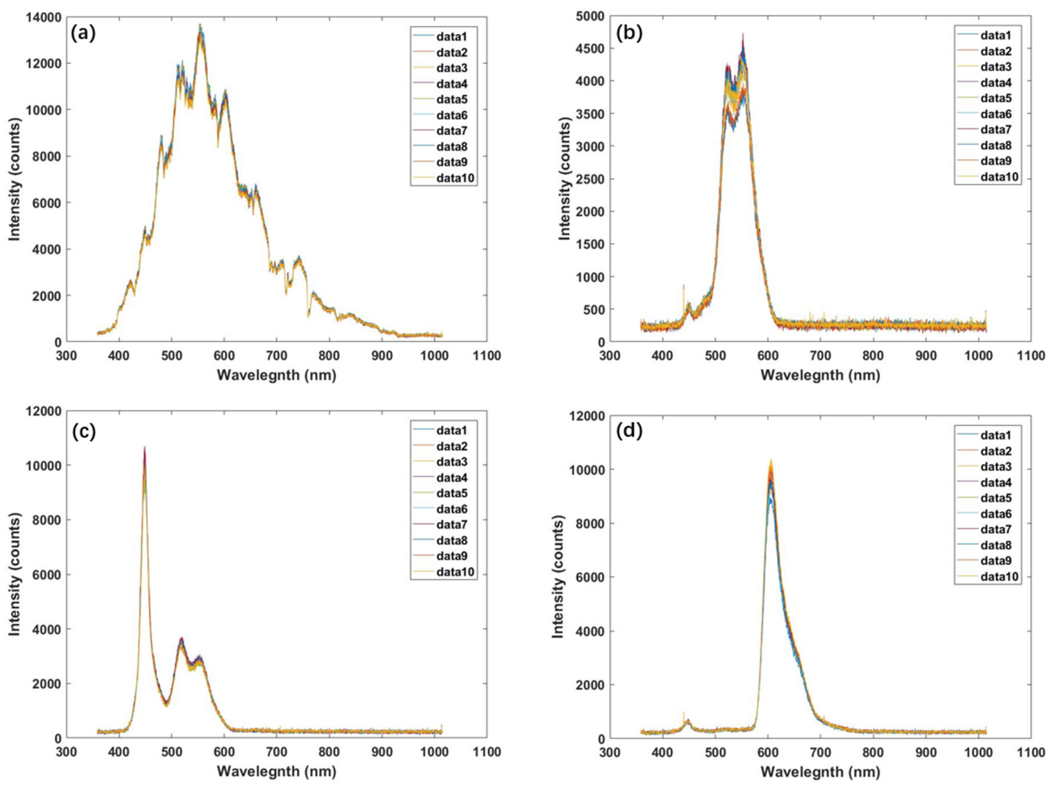
In the second method, we plot the whole spectrum of the same 10 groups of data on one graph and distinguish them by different colors. As shown in Figure 3, we can clearly see two points: one is that the spectral images of 10 groups of similar data almost coincide; the other is that the spectra of sunlight, blue light, green light, and red light shown in the figure are very classic and do not violate the laws of nature. The above phenomenon shows that the measurement accuracy of the hyperspectral imaging system is high, and the detection ability of each band light is excellent, and the whole system has good stability.
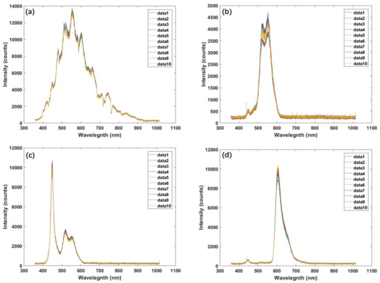
Figure 3.
(a) 10 sets of sunlight spectrum data collected every 10 s. (b) 10 sets of screen green light spectrum data collected every 10 s; (c) 10 sets of screen blue light spectrum data collected every 10 s; (d) 10 sets of screen red light spectrum data collected every 10 s.
We discussed the edge computing technology under IoT combined with deep learning algorithms to realize street garbage classification, fabric defect detection, et al. We wanted to use edge computing technology combined with deep learning algorithms, to classify more spectral data. The current mainstream spectral data processing algorithm is still for one-dimensional spectral data analysis. The machine learning image processing methods widely used in these processing methods are incompatible. As mentioned previously, the current deep learning algorithms are very in-depth in image processing research, these algorithms have relatively high processing efficiency and classification accuracy. If we can preprocess the spectral data, then we use deep learning algorithms for classification, which will greatly improve the efficiency and accuracy of spectral classification.
In our work, we randomly selected five kinds of fruit for testing and achieved accurate classification results through the algorithms. Generally, as long as we obtain enough spectral data and design effective algorithms, we can achieve accurate classification. A large number of literature results have verified the effectiveness of classification based on spectral data. For instance, in [20], the classification based on spectral data was also realized for different algae.
In this paper, we designed a portable optical fiber spectrometer with a screen and verified the stability, accuracy, and detection ability of the system through two different experimental processing methods shown in Figure 2 and Figure 3. We used the spectrometer to collect one-dimensional reflectance spectrum data from five fruit samples, then we reshaped the spectral data structure and transformed it into 2D spectral data. We used our proposed CNN algorithm to extract and classify the 2D spectral image data of five samples. Its maximum classification accuracy rate was 94.78%, and the average accuracy rate was 92.94%, which is better than the traditional AlexNet, Unet, and SVM. Our method makes the spectral data analysis compatible with the deep learning algorithm and implements the deep learning algorithm to process the reflection spectral data from the optical fiber spectrometer.
The remaining paper is organized as follows: Section 2 introduces the optical detection experiment in brief. Section 3 provides the details of the proposed spectral classification method. Section 4 reports our experiments and discusses our results. Finally, Section 5 concludes the work and presents some insights for further research.
2. Optical Detection Experiment
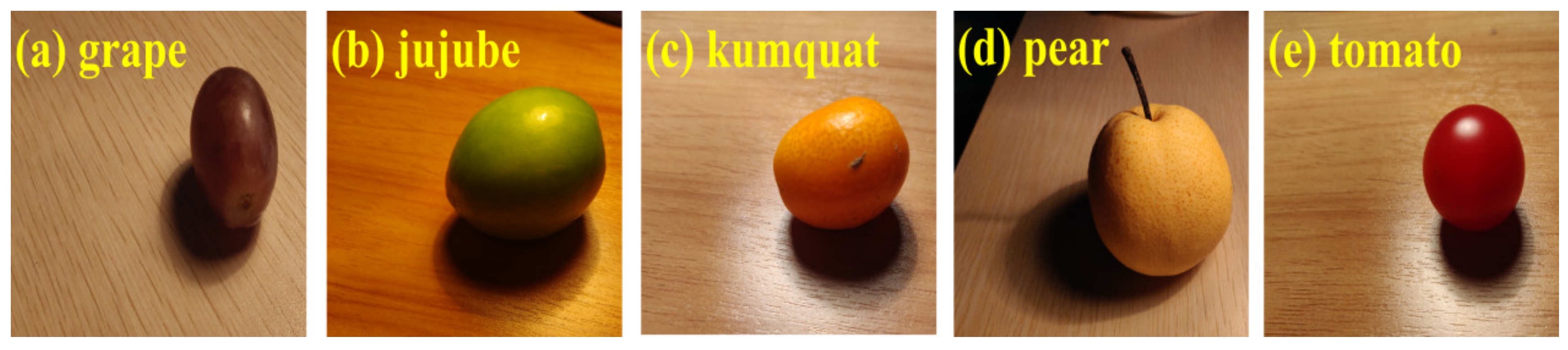
We collected one-dimensional data of grapes, jujubes, kumquats, pears, and tomatoes through a portable optical fiber spectrometer. The pictures of the five samples are presented in Figure 4.
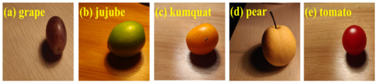
Figure 4.
Experimental samples.
Some reasons will affect remote sensing spectral detection in the real world. For instance, the incident angle and reflection angle of light is not stable in the real optical platform detection environment. Therefore, to adapt to the change of angle, we adjusted the alignment direction of the optical fiber port of the equipment to better achieve the good effect of the optical detection experiment.
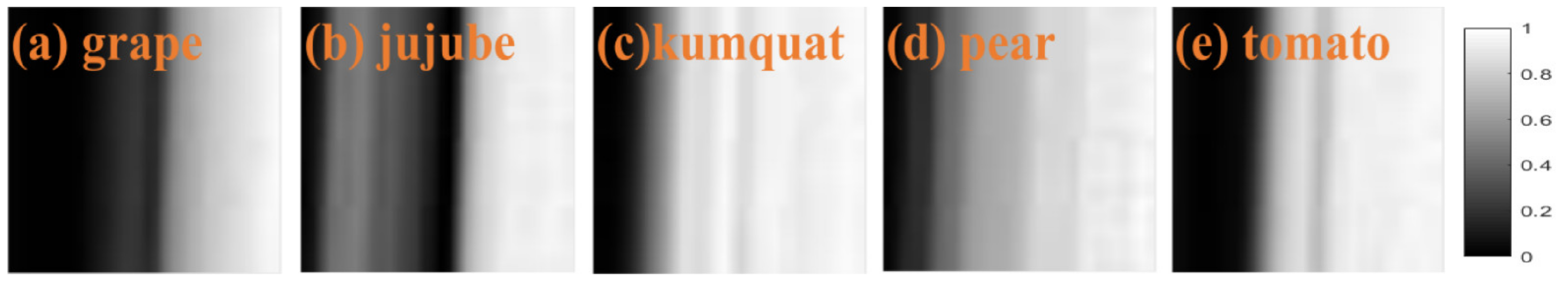
Most two-dimensional images are processed and classified by convolution neural network models. However, the spectral data we obtained through the spectrometer is in a one-dimensional format, which is incompatible with the method of deep learning algorithms to process the 2D spectral data. To transform one-dimensional data into two-dimensional data, to realize the classification of deep learning algorithms, we finished the transformation of the one-dimensional data through the "Reshape" function in Matlab. After processing, we obtained five kinds of two-dimensional spectral data (32 × 32 pixels). These images are presented in Figure 5. In Section 3, we chose a method for deep learning called a convolutional neural network, which classifies these 2D spectral data.

Figure 5.
2D spectral data samples.
3. Proposed Method
3.1. Model Description
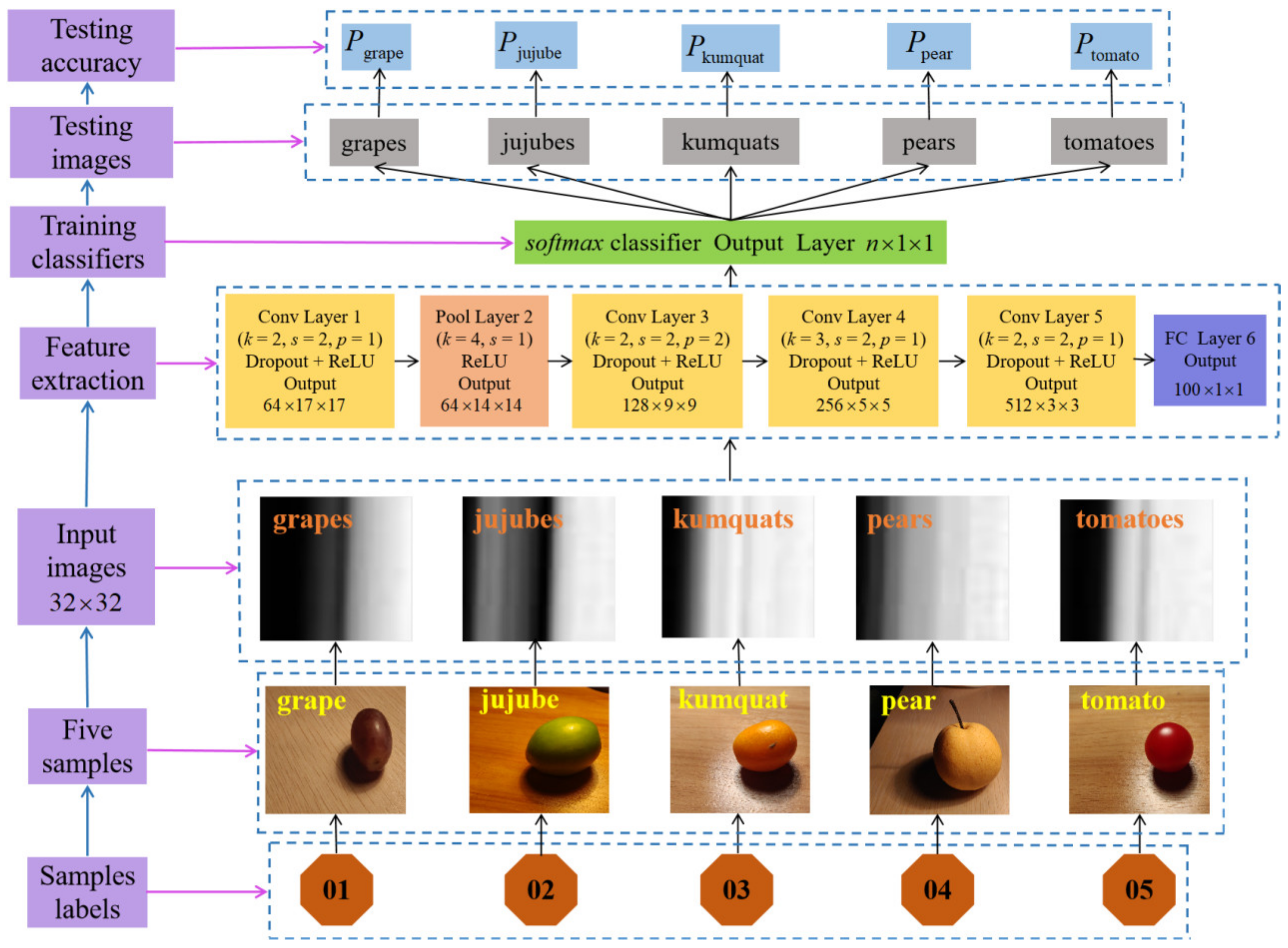
Using a deep learning convolutional neural network model to identify spectral data can be divided into two steps. First, perform feature extraction on the images, and then use the classifier to classify the images. The specific recognition process is depicted in Figure 6.
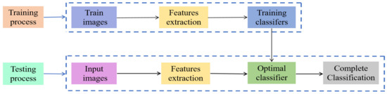
Figure 6.
Convolutional neural networks (CNN) recognition process.
In general, there are convolutional layers, pooling layers, and fully connected layers in a convolutional neural network architecture. Compared with other deep learning models, CNNs show better classification performance.
When CNNs perform convolution operations, the image feature size of the upper layer is calculated and processed through convolution kernels, strides, filling, and activation functions. The output and the input of the previous layer establish a convolution relationship with each other. The convolution operation of feature maps uses the following formula.
where is the activation function, is the output value of the i-th neuron in the (l − 1)-th layer, represents the weight value of the i-th neuron of the l-th convolutional layer connected to the j-th neuron of the output layer, represents the bias value of the j-th neuron of the l-th convolutional layer.
where is the activation function, represents the downsampling function, is the constants used when the feature map performs the sampling operation, represents the bias value of the j-th neuron of the l-th convolutional layer.
The convolutional neural network is usually equipped with a fully connected layer in the last few layers. The fully connected layer normalizes the features after multiple convolutions and pooling. It outputs a probability for various classification situations. In other words, the fully connected layer acts as a classifier.
The Dropout [21] technology is used in CNN to randomly hide some units so that they do not participate in the CNN training process to prevent overfitting. The convolutional layer without the Dropout layer can be calculated using the following formula.
The mean of w, b, and is the same as that of Equation (1).
The discard rate with the Dropout layer can be described as (5):
In fact, the Bernoulli function conforms to the distribution trend of Bernoulli. Through the action of the Bernoulli distribution, the Bernoulli function is randomly decomposed into a matrix vector of 0 or 1 according to a certain probability. Where r is the probability matrix vector obtained by the action of the Bernoulli function. In the training process of models, it is temporarily discarded from the network according to a certain probability, that is, the activation site of a neuron no longer acts with probability p (p is 0).
We multiply the input of neurons by Equation (5) and define the result as the input of neurons with the discard rate. It can be described as.
Therefore, the output was determined using the following formula.
Here, k represents the number of the output neurons.
In this work, we classified 2D spectral data using AlexNet. However, the recognition rate was not high. Mainly, the reasons were analyzed as follows:
- (1)
- Due to the small amount of spectral data sample set collected in this experiment, the training data sets are difficult to meet the needs of deeper AlexNet for feature extraction, learning, and processing. Therefore, the traditional network architecture needed to be streamlined.
- (2)
- In the convolutional process, the more times of convolution, the more spectral features can be fully extracted. The process also uses a large number of convolution kernels, which will bring difficulties to the calculation. The long stride affected the classification accuracy, it was necessary to decrease the traditional parameters of the network convolutional layer.
- (3)
- If a wrong pooling method was used, it would decrease the efficiency of the network learning features and the accuracy of targets classification. The traditional network pooling layer needed to be reduced.
Therefore, we simplified the traditional AlexNet network architecture, decreased the parameters of the convolutional layers, reduced the number of pooling layers, and proposed a new CNN spectral classification model. Figure 7 reveals a specific deep learning spectral classification model framework. Additionally, we added a Dropout layer after each convolutional layer, k represents the size of convolution kernels or pooling kernels, s is the step size moved during convolution or pooling in the CNN operation, and p represents the value of filling the edge after the convolutional layer operation, and generally, the filling value is 0, 1, and 2.
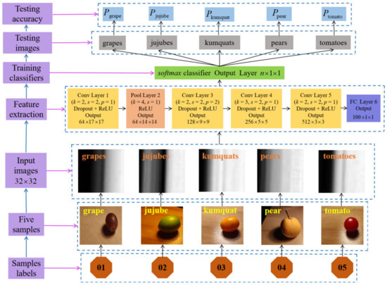
Figure 7.
Deep learning spectral classification model framework diagram.
Since the CNN model requires images of uniform size as input, all spectral data images are normalized to a size of 32 × 32 as input images. We divided the spectral data into n categories, so in the seventh layer, after the Dropout layer and the activation function softmax were calculated, n × 1 × 1 neurons were output, that is, the probability of the category where the n nodes were located.
3.2. Dropout Selection Principle
Dropout can be used as a kind of trick for training convolutional neural networks. In each training batch, it reduces overfitting by ignoring half of the feature detectors. This method can reduce the interaction in feature hidden layer nodes. In brief, Dropout makes the activation value of a certain neuron stop working with a certain probability p when it propagates forward.
In a deep learning model, if the model has too many parameters and too few training samples, the trained model is prone to overfitting. When we train neural networks, we often encounter overfitting problems. The model has a small loss function on the training data and a high prediction accuracy. The loss function on the test data is relatively large, and the prediction accuracy rate is low. If the model is overfitted, then the resulting model is almost unusable. Dropout can effectively alleviate the occurrence of over-fitting and achieve the effect of regularization to a certain extent. The value of the discard rate plays an important role in the deep learning model. An appropriate Dropout value can reduce the complex co-adaptation relationship between neurons and makes the model converge quickly.
In the training process of CNNs, when the steps of the convolution operation are different, the number of output neurons is different, which will reduce their dependence and correlation. If we quantify the correlation, it will increase the dependence. Therefore, we set the discard rate to narrow the range of correlation. After we successively take values in the narrow range, we train and predict the network model again. It will make any two neurons in different states have a higher correlation and improves the recognition accuracy of the model.
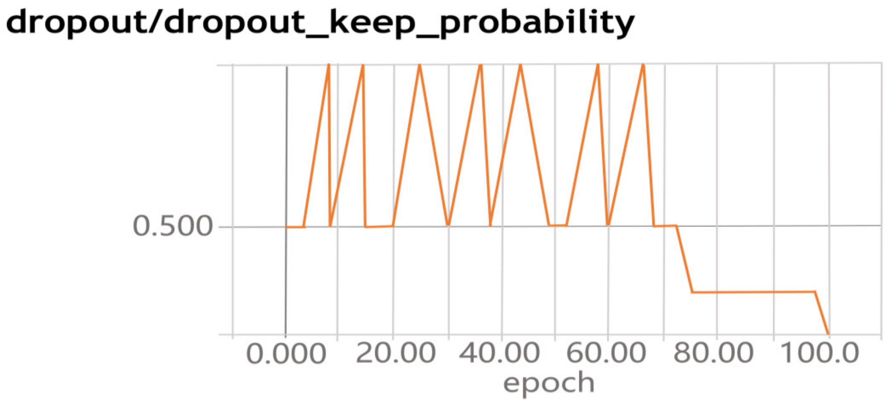
When we trained our proposed CNN model, we visualized the movable trend in dropout layers. Figure 8 presents the movable trend. Figure 8 demonstrates that it is very unstable between 0.5 and 1, which is prone to over-fitting. In (0, 0.1) and (0.2, 0.5), when increasing the epoch, the discard rate drops rapidly, and it is prone to under-fitting. In (0.1, 0.2), the discard rate gradually tends to a stable and convergent state, it is indicated that the value is more appropriate in the interval.

Figure 8.
Dropout change graph.
4. Experimental Results and Discussion
In the algorithms’ experiments, our hardware platform was: CPU frequency 3.00 GHz, the 32 GB memory, a GTX 1080ti GPU graphics card, and the Cuda 9.2 (Cudnn 7.0) accelerator. Our software platform was Keras 2.2.4, TensorFlow 1.14.0, Anaconda 3 5.2.0, Spyder, and Python 3.7 under win10 and a 64-bit operating system.
4.1. Data Distribution
In the experiments of the algorithm classification, the 2D spectral data of five fruit samples were obtained from the optical detection experiment. We divided the 2D spectral data into the training set, the verification set, and the testing set. The number of the training sets is about three times that of the testing set. Results are shown in Table 1.

Table 1.
The data set.
4.2. Train Results
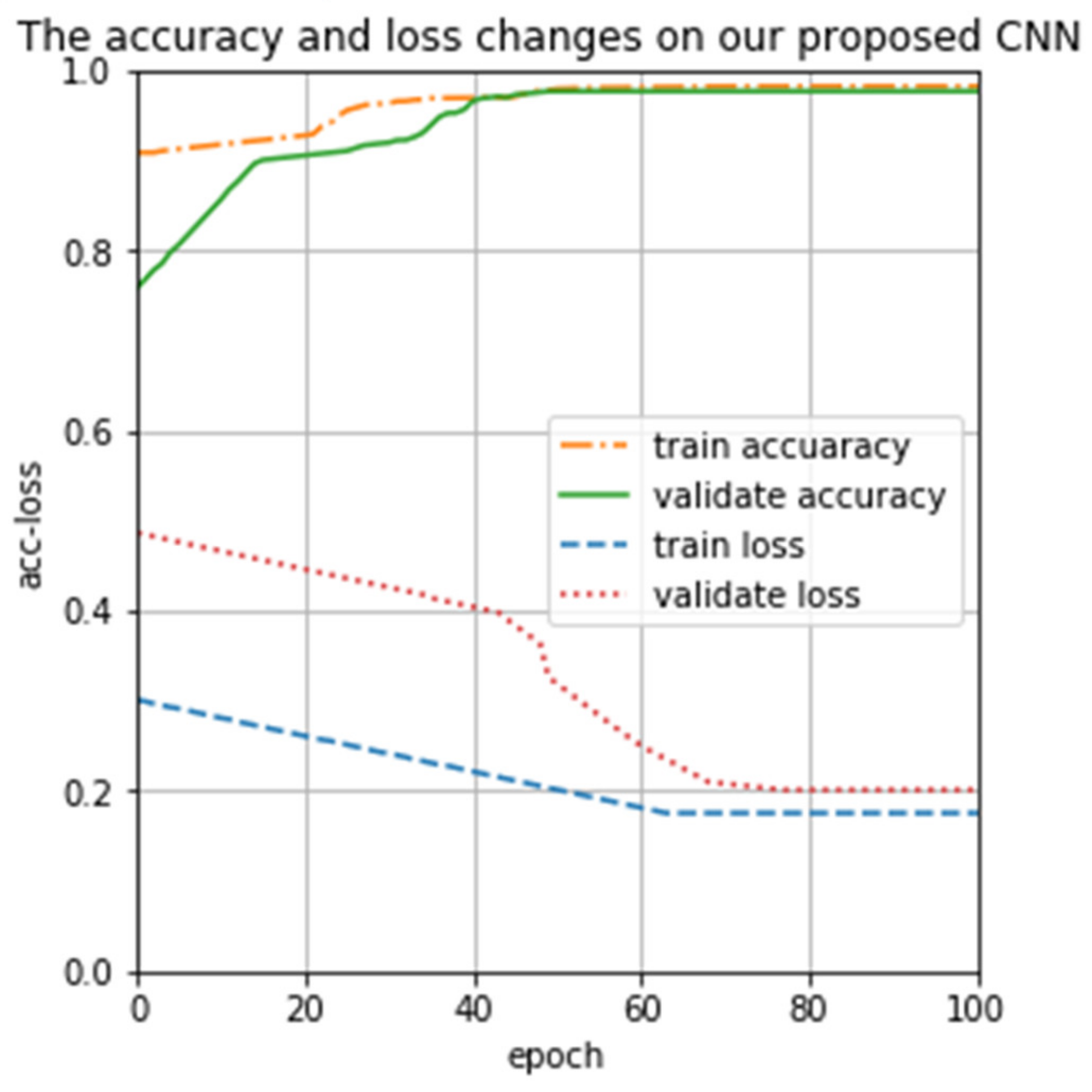
We trained our proposed CNN model, and the results are presented in Figure 9. From Figure 9 we can see that the loss of the training set and the validation set is always between 0.1 and 0.5, and there are no irregular up-and-down violent fluctuations. Both the training accuracy and the validating accuracy are rising and eventually reach a stable value; there is no longer a trend of large value changes. It can find out that if we increase the epoch, the training loss and the validating loss gradually become smaller, and eventually stabilizes. To sum up, our proposed CNN can overcome vanishing gradient in the process of training and validating, and can fully extract features of spectral data from end to end, which is conducive to the correct classification of spectra
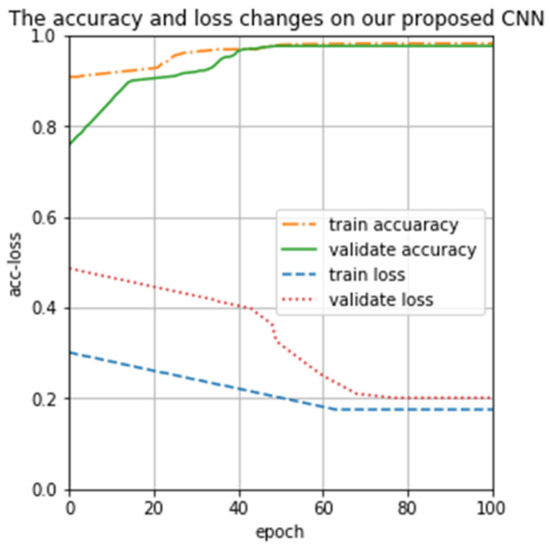
Figure 9.
Proposed CNN iteration training change graph.
Through the model’s training time, accuracy, and loss curve, we can comprehensively judge the performance of the model. If the model consumes less training time, the accuracy and loss curves also tend to be stable and fast, and it is illustrated that the model has good convergence performance in a short time. If the model consumes for a long time, the accuracy and loss curve also tends to be steady and slow, and this indicates that the model has poor performance. Through the length of time consumed and the change in accuracy loss, some parameters of the model such as learning rate, batch processing times, etc, can be fine-tuned to improve the performance of the model. Therefore, we not only consider the model’s accuracy and loss changes to the training data, but also consider the time consumption.
We recorded the time of training 100 times under four algorithms, Table 2 reveals the time of the four algorithms.
Table 2.
Training time.
As shown in Table 2, our proposed method consumes the least time. It is proved that our proposed method can adapt to the feature extraction of spectral data, and does not bring too much parameters calculation to occupy memory.
4.3. Test Results
The SOTA image recognition model ViT-G/14 uses the JFT-3B data set containing 3 billion images, and the amount of parameters is up to 2 billion. On the ImageNet image data set, it achieved a Top-1 accuracy of 90.45%, it has surpassed the Meta Pseudo Labels model. Although ViT-G/14 performs well in addition to better performance, our data volume and categories are limited. Our data cannot adapt to the parameter training and testing of the SOTA image recognition model ViT-G/14 with more categories and large amounts of data. Therefore, we chose AlexNet, Unet, SVM, and our proposed CNN for comparison.
When epochs are set as 100, the testing accuracy of four algorithms under different parameters is presented in Table 3. Table 3 reports that different parameters correspond to different testing accuracy. For instance, the inputting shape is a batch size of 32, the learning rate is 0.001, the optimizer is SGD, our testing accuracy is 92.57%. It is superior to other parameters. Furthermore, the testing accuracy obtained by the values of different parameters also shows that our proposed CNN achieves an improvement in the classification accuracy of 22.86% when compared to AlexNet.
Table 3.
Test accuracy under different parameters.
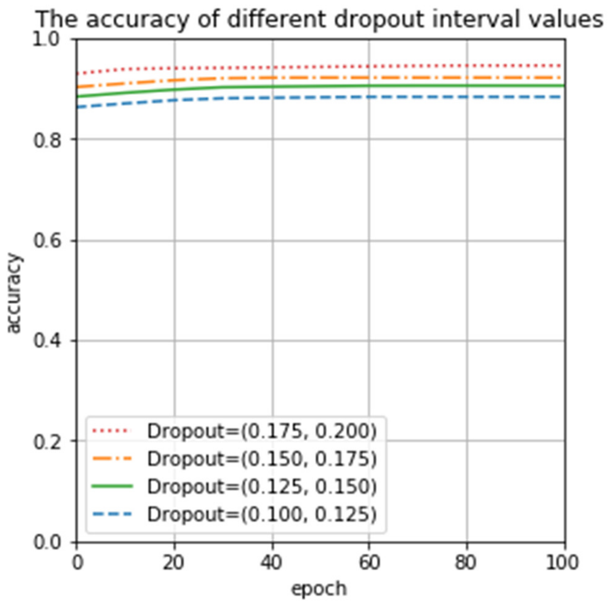
Figure 8 illustrates that the discard rate is the most appropriate value in (0.1, 0.2). We divided it into four sub-intervals to test the precision of our proposed CNN. Testing results are revealed in Figure 10. The results in Figure 10 demonstrate that the accuracy in (0.175, 0.200) is higher than in (0.100, 0.125), (0.125, 0.150), and (0.150, 0.175). Evidently, our proposed CNN model has the best performance in (0.175, 0.200), it verifies the correctness of the dropout discard rate analysis and selection principle simultaneously in Section 3.2.
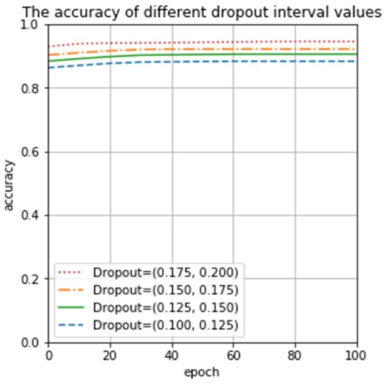
Figure 10.
Accuracy in different intervals.
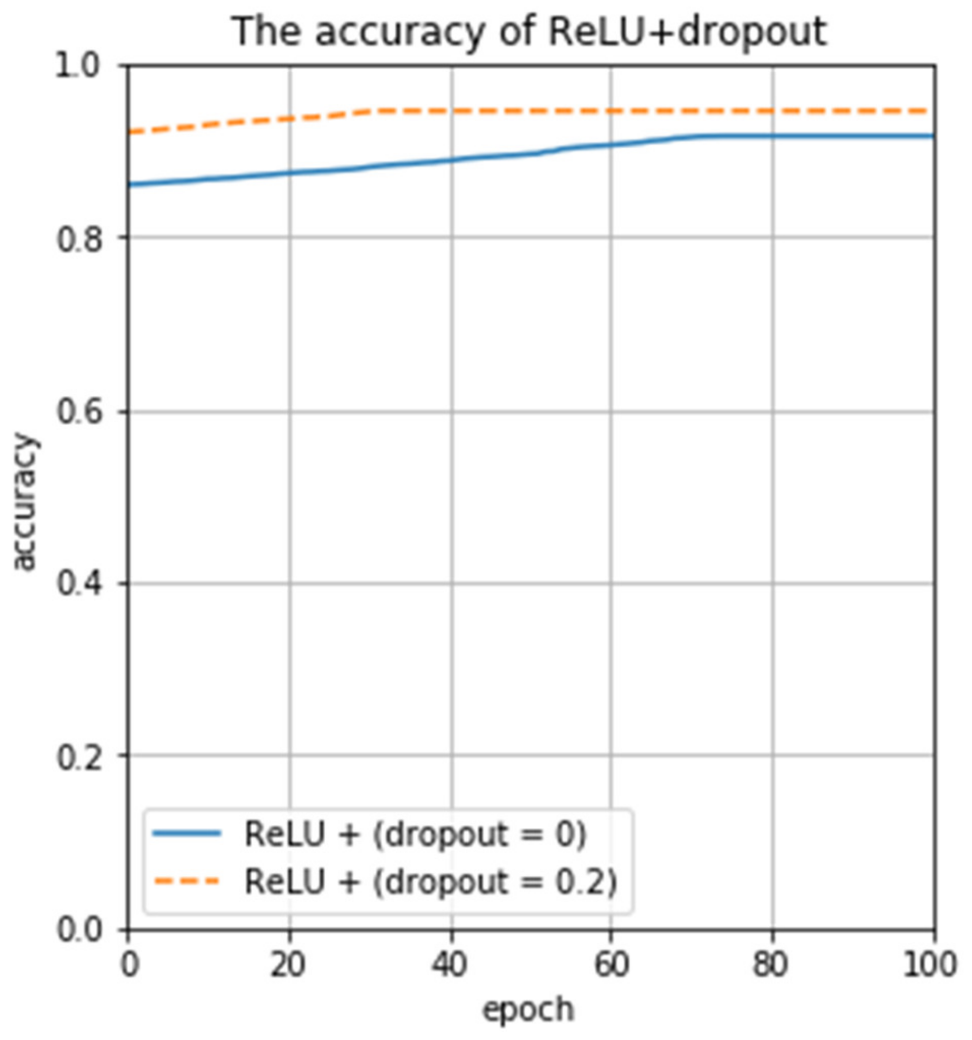
To verify the feasibility of ReLU and the discard rate in this work, we again used ReLU with the Dropout layer (dropout = 0.2) and without the Dropout layer (dropout = 0) for testing. Testing results are shown in Figure 11. The experimental results confirm that the recognition rate is as high as 94.57% when ReLU is used and the discard rate is 0.2, which is significantly higher than the recognition result without the dropout layer (dropout = 0). In summary, our proposed CNN model outperforms AlexNet and SVM tested in terms of classification accuracy, and it can perform accurate spectral classification.
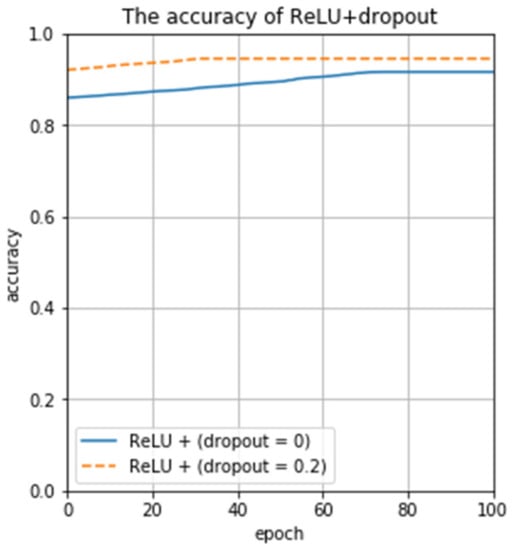
Figure 11.
The impact of the dropout value on the recognition rate.
As shown in Table 4, the testing time of our proposed CNN is lower than AlexNet, Unet, and SVM. Evidently, our proposed model can quickly extract two-dimensional spectral features and gives the prediction result in the testing process.
Table 4.
Testing times using four different methods.
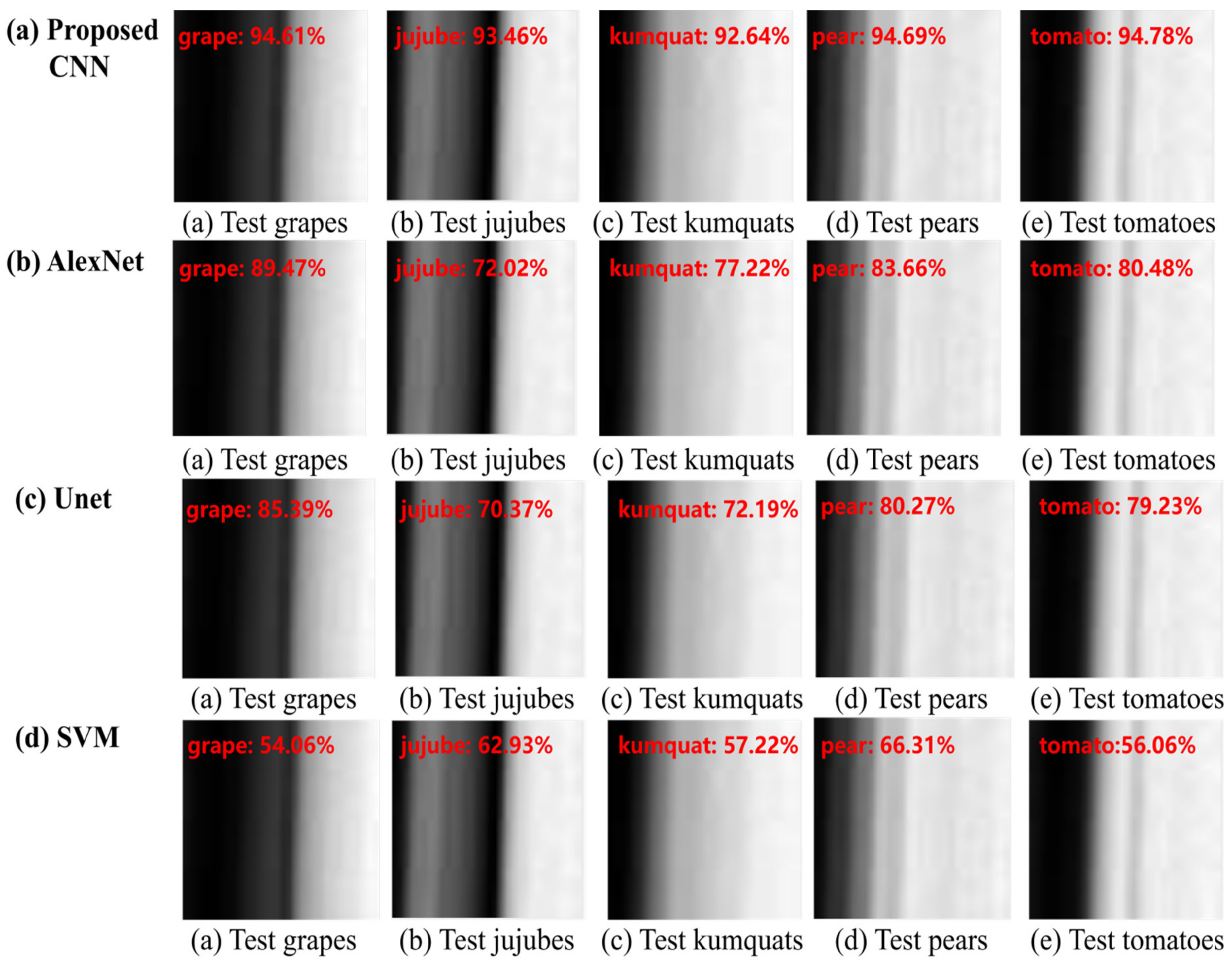
To compare the performance of four different classification methods, we tested five samples one by one. Table 5, Table 6, Table 7 and Table 8 show testing results. Table 5, Table 6, Table 7 and Table 8 report that the testing precision of our proposed CNN is superior to AlexNet, Unet, and SVM. Therefore, our proposed CNN model has strong robustness to 2D spectral data.
Table 5.
Testing five samples with our proposed CNN.
Table 6.
Testing five samples with AlexNet.
Table 7.
Testing five samples with Unet.
Table 8.
Testing five samples using the support vector machine (SVM).
In Section 4.2, we considered the model training time, we also consider the speed of the model during testing images, simultaneously. If we proposed model is slower on testing image speed, it is revealed that the performance of the model does not take into account. The quality of a model not only depends on its training time, training accuracy, and verification accuracy, etc, but also its testing accuracy and testing time.
Figure 12 shows the maximum testing precision of each sample under four different algorithms. It can figure out if the testing effect of our proposed CNN is significantly greater than the other three methods in Figure 12. Obviously, our proposed CNN has high classification precision and generalization ability to 2D spectral data.
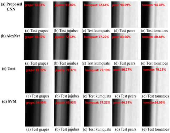
Figure 12.
(a) The maximum testing results of the proposed CNN are between 90% and 95%. (b,c) The maximum testing results of AlexNet and Unet are between 70% and 90%. (d) The maximum testing results of the SVM are between 50% and 70%.
5. Conclusions
In this work, a new CNN architecture was designed to effectively classify 2D spectral data of five samples. Specifically, we added a Dropout layer behind each convolutional layer of the network to randomly discard some useless neurons and effectively enhance the feature extraction ability. In this way, the features uncovered by the network became stronger, which eventually lead to a reduction of the network architecture parameters calculation complexity and, therefore, to a more accurate spectral classification. The experimental comparisons conducted in this work shows that our proposed approach exhibits competitive advantages with respect to AlexNet, Unet, and SVM classification methods. Although fiber optic spectrometers cannot directly perform spectral imaging classification research, our work has confirmed that deep learning algorithms can be combined with the spectral data obtained by the optical fiber spectrometer for classification research. We will use fiber optic spectrometers to obtain more samples of spectral data and combine edge computing technology to send to the deep learning model for data processing and classification research in the future.
Author Contributions
Conceptualization, L.X. and F.C.; methodology, L.X., F.C. and J.W.; software, L.X. and F.C.; validation, L.X., J.X. and J.W.; formal analysis, L.X., F.C. and J.W.; data curation, L.X. and J.X.; writing—original draft preparation, L.X., F.C. and J.W.; writing—review and editing, L.X., F.C. and J.W.; supervision, J.W.; funding acquisition, F.C. and J.W. All authors have read and agreed to the published version of the manuscript.
Funding
This work is supported by National Key Research and Development Program of China (No. 2018YFC1407505); National Natural Science Foundation of China (No. 81971692); the Natural Science Foundation of Hainan Province (No. 119MS001) and the scientific research fund of Hainan University (No. kyqd1653).
Conflicts of Interest
The authors declare no conflict of interest.
References
- Li, L.; Ota, K.; Dong, M. When weather matters: IoT based electrical load forecasting for smart grid. IEEE Commun. Mag. 2017, 55, 46–51. [Google Scholar] [CrossRef] [Green Version]
- Kim, H.Y.; Kim, J.M. A load balancing scheme based on deep learning in IoT. Clust. Comput. 2017, 20, 873–878. [Google Scholar] [CrossRef]
- Alsheikh, M.A.; Niyato, D.; Lin, S.; Tan, H.-P.; Han, Z. Mobile big data analytics using deep learning and apache spark. IEEE Netw. 2016, 30, 22–29. [Google Scholar] [CrossRef] [Green Version]
- Liu, J.; Guo, H.; Nishiyama, H.; Ujikawa, H.; Suzuki, K.; Kato, N. New perspectives on future smart FiWi networks: Scalability, reliability, and energy efficiency. IEEE Commun. Surv. Tutor. 2017, 18, 1045–1072. [Google Scholar] [CrossRef]
- Sun, X.; Ansari, N. EdgeIoT: Mobile edge computing for the Intemet of Things. IEEE Commun. Mag. 2016, 54, 22–29. [Google Scholar] [CrossRef]
- Zhu, Z.; Han, G.; Jia, G.; Shu, L. Modified DenseNet for Automatic Fabric Defect Detection with Edge Computing for Minimizing Latency. IEEE Internet Things J. 2020, 7, 9623–9636. [Google Scholar] [CrossRef]
- Pan, D.; Liu, H.; Qu, D.; Zhang, Z. CNN-Based Fall Detection Strategy with Edge Computing Scheduling in Smart Cities. Electronics 2020, 9, 1780. [Google Scholar] [CrossRef]
- Ping, P.; Xu, G.; Kumala, E.; Xu, G. Smart Street Litter Detection and Classification Based on Faster R-CNN and Edge Computing. Int. J. Softw. Eng. Knowl. Eng. 2020, 30, 537–553. [Google Scholar] [CrossRef]
- Sahni, Y.; Cao, J.; Yang, L.; Ji, Y. Multi-Hop Multi-Task Partial Computation Offloading in Collaborative Edge Computing. IEEE Trans. Parallel Distrib. Syst. 2020, 32, 1133–1145. [Google Scholar] [CrossRef]
- Khaliq, K.A.; Chughtai, O.; Shahwani, A.; Qayyum, A.; Pannek, J. Road Accidents Detection, Data Collection and Data Analysis Using V2X Communication and Edge/Cloud Computing. Electronics 2019, 8, 896. [Google Scholar] [CrossRef] [Green Version]
- Dou, W.; Zhao, X.; Yin, X.; Wang, H.; Luo, Y.; Qi, L. Edge Computing-Enabled Deep Learning for Real-time Video Optimization in IIoT. IEEE Trans. Ind. Inform. 2020, 17, 2842–2851. [Google Scholar] [CrossRef]
- Zhou, Z.; Liu, Q.; Fu, Y.; Xu, X.; Wang, C.; Deng, M. Multi-channel fiber optical spectrometer for high-throughput characterization of photoluminescence properties. Rev. Sci. Instrum. 2020, 91, 123113. [Google Scholar] [CrossRef]
- Markvart, A.; Liokumovich, L.; Medvedev, I.; Ushakov, N. Continuous Hue-Based Self-Calibration of a Smartphone Spectrometer Applied to Optical Fiber Fabry-Perot Sensor Interrogation. Sensors 2020, 20, 6304. [Google Scholar] [CrossRef] [PubMed]
- Yan, L.; Song, Y.; Liu, W.; Lv, Z.; Yang, Y. Phosphor thermometry at 5 kHz rate using a high-speed fiber-optic spectrometer. J. Appl. Phys. 2020, 127, 124501. [Google Scholar] [CrossRef]
- Cai, F.; Wang, T.; Wu, J.; Zhang, X. Handheld four-dimensional optical sensor. Optik 2020, 203, 164001. [Google Scholar] [CrossRef]
- Praveen, B.; Menon, V. Study of Spatial–Spectral Feature Extraction Frameworks with 3-D Convolutional Neural Network for Robust Hyperspectral Imagery Classification. IEEE J. Sel. Top. Appl. Earth Obs. Remote Sens. 2020, 14, 1717–1727. [Google Scholar] [CrossRef]
- Anthony, M.; Wang, Z. Hyperspectral Image Classification Using Similarity Measurements-Based Deep Recurrent Neural Networks. Remote Sens. 2019, 11, 194. [Google Scholar] [CrossRef] [Green Version]
- Li, J.; Xi, B.; Li, Y.; Du, Q.; Wang, K. Hyperspectral Classification Based on Texture Feature Enhancement and Deep Belief Networks. Remote Sens. 2018, 10, 396. [Google Scholar] [CrossRef] [Green Version]
- Liu, X.; Jiang, Z.; Wang, T.; Cai, F.; Wang, D. Fast hyperspectral imager driven by a low-cost and compact galvo-mirror. Optik 2020, 224, 165716. [Google Scholar] [CrossRef]
- Xu, Z.; Jiang, Y.; Ji, J.; Forsberg, E.; Li, Y.; He, S. Classification, identification, and growth stage estimation of microalgae based on transmission hyperspectral microscopic imaging and machine learning. Opt. Express 2020, 28, 30686–30700. [Google Scholar] [CrossRef]
- Hahn, S.; Choi, H. Understanding dropout as an optimization trick. Neurocomputing 2020, 398, 64–70. [Google Scholar] [CrossRef] [Green Version]


Publisher’s Note: MDPI stays neutral with regard to jurisdictional claims in published maps and institutional affiliations. |
© 2021 by the authors. Licensee MDPI, Basel, Switzerland. This article is an open access article distributed under the terms and conditions of the Creative Commons Attribution (CC BY) license (https://creativecommons.org/licenses/by/4.0/).