
Inferring the Hidden Cascade Infection over Erdös-Rényi (ER) Random Graph


School of Computing, Gachon University, Seongnam-si 13120, Korea
Electronics 2021, 10(16), 1894; https://doi.org/10.3390/electronics10161894
Submission received: 9 June 2021
/
Revised: 29 July 2021
/
Accepted: 4 August 2021
/
Published: 6 August 2021
(This article belongs to the Special Issue Multimedia Systems and Signal Processing)
Abstract
:Finding hidden infected nodes is extremely important when information or diseases spread rapidly in a network because hints regarding the global properties of the diffusion dynamics can be provided, and effective control strategies for mitigating such spread can be derived. In this study, to understand the impact of the structure of the underlying network, a cascade infection-recovery problem is considered over an Erdös-Rényi (ER) random graph when a subset of infected nodes is partially observed. The goal is to reconstruct the underlying cascade that is likely to generate these observations. To address this, two algorithms are proposed: (i) a Neighbor-based recovery algorithm (NBRA()), where is a control parameter, and (ii) a BFS tree-source-based recovery algorithm (BSRA). The first one simply counts the number of infected neighbors for candidate hidden cascade nodes and computes the possibility of infection from the neighbors by controlling the parameter . The latter estimates the cascade sources first and computes the infection probability from the sources. A BFS tree approximation is used for the underlying ER random graph with respect to the sources for computing the infection probability because of the computational complexity in general loopy graphs. We then conducted various simulations to obtain the recovery performance of the two proposed algorithms. As a result, although the NBRA() uses only local information of the neighboring infection status, it recovers the hidden cascade infection well and is not significantly affected by the average degree of the ER random graph, whereas the BSRA works well on a local tree-like structure.
1. Introduction
Recently, computer viruses, infectious diseases, and the spread of information have become universal occurrences in various types of networks. As examples, COVID-19 is transmitted from person to person, whereas certain rumors have spread over the Internet through the development of social network services, such as Facebook and Twitter. Given such circumstances, it is important to quickly prevent the spread of rumors, malicious information, or viruses through observations. In practice, however, the observation of such spreading events is often incomplete because some nodes or individuals are reluctant to reveal their infection status [1]. Hence, inferring a hidden infection may provide some hints regarding the global properties of the diffusion dynamics [2,3]. Furthermore, it often opens up effective control strategies for the optimal dissemination or mitigation of spread. The research on inferring hidden nodes and structures has recently received significant attention. Netrapalli et al. [4] considered the graph inferring problem, where only the infection times of the nodes are given. In this study, they tried to estimate which neighbors were influential based on multiple cascades spreading through the graph. To do this, they suggested a Maximum Likelihood Estimator (MLE) for recovering influential connections, which guarantees a necessary cascade sample complexity for an Independent Cascade (IC) model. Sundareisan et al. [5] investigated the problem of recovering missing infected nodes and the source nodes of an epidemic. For this, they proposed an algorithm called NETFILL, which solves these two inference problems simultaneously. In addition, Xiao et al. [6] considered a problem for reconstructing the underlying cascade that is likely to generate observations of infection in the graph. They estimated the infection probabilities by generating a sample of the probable cascades, and proposed several algorithms for sampling directed Steiner trees with a given set of terminals. However, it is known [6] that inferring a hidden infected node is extremely difficult, even if the network structure is given. This is because it is necessary to first identify the path through which an arbitrary node is infected in the graph, despite the potential of an exponential number of paths. It is also known [7] that finding a hidden infected node that has not yet been observed is still a difficult problem even if some information regarding which node is infected and when such infection occurred is given. Hence, many prior studies have considered some of the greedy approaches to sampling a candidate infection graph using Steiner tree sampling [6,7]. An Expectation-Maximization (EM) approach applied under a partial observation scenario was also investigated in Reference [8]. He et al. [9] proposed an algorithm that effectively recovers a graph with partial cascade samples by considering a generative model, which is referred to as a Multi-Cascaded Model (MCM). In addition, Choi et al. [10] investigated the classification of causes of infection (random infection versus cascade infection) in a network under a partial observation of the infection status. To do this, they also considered the hidden cascade recovery approach in their proposed iterative classification algorithm. However, only a tree structure has been studied due to its computational complexity. There have been several studies conducted on fault detection as a hidden infection node in a communication network system. Huang et al. [11] investigated the VINI testbed, which supports the choice of paths to monitor, detect, and confirm the existence of a failure, correlating multiple independent observations in a single failure event. Tosic et al. [12] studied the problem of distributed sensor failure detection in networks with a small number of defective sensors, whose measurements differ significantly from the neighboring measurements. Furthermore, some hidden state estimation problems [13,14] have been investigated for sliding mode control. Although these prior studies were conducted on various synthetic or real graphs, there have been a few studies on how the recovering tendency changes when the actual graph changes according to arbitrary parameters. However, this is an important problem in terms of suggesting how to control the spreading cascade when the degree of recovery varies significantly depending on the parameters of the graph.
Hence, in this paper, the recovering problem of a hidden cascade node is considered for the Erdös-Rényi (ER) random graph as represented by the average degree . The average degree is the average number of neighbors for all nodes in the graph. Although it is a synthetic graph, an ER random graph may have a local tree-like structure with a large diameter or a very dense graph structure with a small diameter as the parameter varies. Therefore, as a first step, we study the recovery performance according to the parameter for a relatively simple ER random graph rather than other real-world graphs in References [6,7]. The objective is to develop efficient algorithms that find hidden infected nodes in this parameterized ER random graph and to show how the recovery performance changes as the parameter changes.
The main contributions of this study can be summarized in more detail as follows:
- First, the recovering hidden cascade infection problem is studied on the well-known ER random graph under the IC model. As shown in Figure 1, for a given number of nodes, the shape of the ER random graph varies greatly depending on the average degree . Hence, the effect of this parameter on the recovery performance was investigated for the first time.
- Second, to solve the problem, an algorithm that detects whether the node is infected with only neighboring infection information is first designed, which gives the local infection status of the graph. For this, the possibilities that can occur with the infected neighbor nodes are parameterized by a single parameter, and the method of selecting the best parameter is investigated. Next, as global information regarding infection, an efficient algorithm is proposed that uses the location of the estimated cascade sources. The infection probabilities from the sources are used, which is a new method that has yet to be approached.
- Third, various simulations are conducted to obtain the recovering performance of the two proposed algorithms. As a result, although the first one uses only local information of the neighboring infection status, it recovers the hidden cascade infection well compared with other baseline algorithms. Further, it is shown that the detection performance of the second graph is also good if the ER random graph has a local tree structure.
The remainder of this paper is organized as follows. Section 2 discusses related studies. In Section 3, the infection and observation models and the goals of the study are introduced. In Section 4 and Section 5, the neighbor- and BFS tree-source-based recovery algorithms are presented, respectively. In Section 6, the simulation results are presented, and, in Section 7 and Section 8, some concluding remarks and future works are given.
2. Related Work
The related studies are divided into the following two categories: (1) Hidden node (or structure) inference and (2) cascade source detection.
- (1)
- Hidden node (structure) Inference. For the graph structure learning, Netrapalli et al. [4] considered the graph inference problem, where only the infection times of the nodes are given. In this study, the authors tried to estimate which neighbors are influential through multiple cascades spreading throughout the graph. To do this, they suggested a MLE for recovering influential connections, which guarantees a necessary cascade sample complexity for the IC model. Pouget et al. [15] studied the graph structure learning from the sparse recovery framework for a general discrete cascade model. They first formulated the problem as a general Linear Threshold (LT) model and proposed an algorithm that recovers the true edges in the graph with high probability. The authors of Reference [16] considered the graph learning problem for continuous-time cascade models. For this, they first introduced the concept of a trace complexity as the number of distinct traces required to achieve high fidelity in reconstructing the topology of an unobserved network. Based on this, they proposed a simple but efficient algorithm for inferring the graph structures. He et al. [9] proposed an algorithm that effectively recovers a graph with partial cascade samples by considering a generative model, referred to as the MultiCascades Model. As the key idea of this model, it uses the commonality between highly correlated diffusion graphs. He et al. [17] also designed some algorithms inferring the influence function from the partial observations of the node activation in the graph. To do so, they considered a probably approximately correct learnability of the influence functions for the missing observations. Rozenshtein et al. [18] has studied the reconstruction of cascades from partial timestamps. They designed an effective algorithm called a CULT to recover from epidemics by formulating a temporal Steiner tree problem. Xiao et al. [7] formulated a cascade-reconstruction problem as a variant of the Steiner tree problem. With their approach, they first estimate a tree that spans all reported active nodes, which satisfies some temporal consistency constraints. Furthermore, they proposed several algorithms and showed that one of them achieves a linear time -approximation guarantee, where k is the number of active nodes. Some researchers have studied the graph learning without the explicit time of infection. Gripon et al. [19] proposed an algorithm that recovers infection edges, which are the edges in the graph that are involved in the infection process from an unordered set of infected nodes. They designed an algorithm to infer such edges in order by comparing each trace into a path using information in which pairs of nodes in the path co-occur most frequently in the observations. Amin et al. [20] investigated the problem of reconstructing the node connectivity using only the initial source nodes and the final diffusion snapshot of infected nodes for the IC model, without any time information of the nodes. Wu et al. [8] considered an EM approach for the Continuous Independent Cascade (CIC) model using partial information on the infection status of the graph, and proposed algorithms that estimate the influence parameters of edges based on the EM. The authors of Reference [5] investigated the problem of recovering missing infected nodes and the source nodes of an epidemic. To do so, they proposed an algorithm called NETFILL, which solves these two inference problems simultaneously. The authors of Reference [6] considered a problem that reconstructs the underlying cascade that is likely to generate observations of infections in the graph. They estimated the infection probabilities by generating a sample of the probable cascades, proposed several algorithms for sampling directed Steiner trees with a given set of terminals.
- (2)
- Cascade Source Detection. Next, some of the cascade source detection problems are summarized in the following sections. Zhu et al. [21] considered the cascade source detection problem using an ER random graph. They proposed a new source localization algorithm for the IC model, called the Short-Fat Tree algorithm, which selects the node of the Breadth-First Search (BFS) tree, which has the minimum depth but the maximum number of leaf nodes. In addition, they also proposed a new source localization algorithm, called an Optimal-Jordan-Cover (OJC) in Reference [22], which extends the source inferring problem to the case of multiple sources in the graph. The OJC first extracts a subgraph using a candidate selection algorithm that selects the source candidates based on the number of observed infected nodes in their neighborhoods. Considering the heterogeneous SIR diffusion in the ER random graph, they proved that OJC can locate all sources with a probability of 1 asymptotically with partial observations. Next, some studies have utilized partial information on when a random node is infected. The authors of Reference [23] studied the problem of partial timestamps of infection. They solved this problem by formulating a ranking problem on graphs using the likelihood of being the source. In the opposite direction as the previous source detection problem, Fanti et al. [24] first studied how to spread as many anonymous messages as possible while hiding the source. They designed a message-propagation protocol, called an adaptive diffusion model, and then obtained analytical results of the hiding performance of the model. The authors of Reference [25] considered the source-finding problem with observation time information , which contains some set S of nodes with the first infection timestamps . Tang et al. [26] investigated the problem based on the network topology and a subset of infection timestamps. For a tree network, they first derived the maximum likelihood estimator of the source and unknown diffusion parameters. Using this, they considered an optimization over a parametrized family of Gromov matrices in the design of an estimation algorithm for general graphs. Kumar et al. [27] considered a problem with additional relative information about the infection times of a fraction of node pairs.
3. Model and Goal
3.1. Models
- Graph Model. The recovery problem of a hidden cascade node for the ER random graph G, as represented by some graph parameters, is considered. An ER random graph, which is usually denoted by on the vertex set V, is a random graph that connects each pair of nodes with probability . This model is parameterized by the number of nodes, and p. The expected number of degrees of a node is then computed by (see Figure 1). Most results for ER graphs suppose that this is fixed (e.g., or ) or increases slowly (e.g., ). Although it is a synthetic graph, the ER random graph may have a local tree-like structure with a large diameter or an extremely dense graph structure with a small diameter as the parameter varies.
- Cascade and Observation Models. As a cascade model, a well-known independent cascade model is considered. With this model, three possible states of nodes are considered: Susceptible (S), Active (A), or Inactive (I). First, a susceptible state means that a node can be activated. Next, if a node in the susceptible state is activated at the previous time slot, it becomes an active node, which is in a state in which other susceptible child nodes are activated. The inactive state denotes a state in which a node was activated once earlier, but no longer able to activate other susceptible nodes. In the proposed model, the cascade starts from a subset of seed nodes that have been initially infected in the network. The cascade occurs in a discrete round, At round , the seed nodes are active, and the others are inactive. Then, if a node u receives the information or is infected from one of its infected nodes at time t, the node spreads its own information (or a virus) to its neighbor v with probability at the next time . It is assumed that the activated nodes are active for only one time slot, and they become inactive in the next time slot. Once a node becomes inactive, it maintains the state until reaching the end of the cascade process. The process stops when no more nodes are infected. For a simpler expression, the probability is also used, where is the edge among the nodes in the network. When some neighbors are already infected, the probability of infection is regarded as zero. Let be the diffusion vector over each edge An infected node v is considered to report its status of infection with probability , labelled based on an observation probability and denoted as . The node represents the information source, which acts as a node that initiates diffusion, and the set indicates the set of observed (reported) infected nodes. Further, represents the observed snapshot of the cascade graph at time Finally, assume that the number of cascade sources is given as a prior by for a certain analytical tractability. We summarize the explanations of notations used in the paper in Table 1.
3.2. Goal: Estimation of an Infection
The goal of the paper is to recover the hidden (not reported) infected nodes (in the IC model, an infected node indicates both active and inactive nodes), excluding the reported infected nodes . More precisely, for node with the ground truth , the objective is to design an estimator of , denoted by such that , which maps the node to the state of infection with high accuracy. Here, is called based on the recovery function of .
- Performance metric. As a performance measure for the true recovery of the proposed estimation algorithm, the following precision-based accuracy is used: Let be the set of hidden infected nodes (ground truth) and be the estimated recovery set of infected nodes by the estimator . As a measure of the hidden cascade recovery, a precision metric is defined bywhere is an indicator function that has only one function for ; otherwise, it is zero. The notion is the number of infected nodes for . This metric measures the rate at which the number of recovered nodes is truly infected among the estimated recovered set for the observed snapshot at time . To obtain this, two classification algorithms are proposed. The first is a neighbor-based approach that uses local infection status information. The second approach is a source-location-based approach that uses global infection status information from the cascade source nodes. Various simulations are then conducted, and the results are obtained by varying the model parameters described in Section 6.
4. Neighbor-Based Recovery Algorithm
In this section, a naive approach is first introduced that uses the number of infected neighbor nodes to recover the hidden infection. As the motivation of this approach, if there are many infected neighbors of a node v, it also has a high probability of being infected. However, it is known that Reference [6] is an highly complicated task to determine which path the infection has progressed along when centring on a single node. Therefore, in the following subsection, a simple but efficient algorithm is proposed that estimates whether node v is infected, based on the degree of infection around it.
Neighbor-Based Recovery
In the neighbor-based recovery algorithm, called NBRA(), the main idea is to properly consider the possibility that a node is infected from already infected nodes. The detailed description of this is as follows.
- Algorithm. In NBRA(), the algorithm first initializes the recovering set as an empty set. Then, for the nodes , it counts the number of observed infected neighbor nodes, denoted by , and sets the minimum diffusion probability among by . Next, a heuristic infection probability is defined from the infected neighbor nodes of node v. In this algorithm, the probability is set to zero when there are no infected neighbor nodes, i.e., Otherwise, it setswhere is a trade-off parameter. Finally, the algorithm puts the node v into the recovering set if the probability is greater than (this approach implies that, if the heuristic infection probability from the infected neighbor nodes is larger than , it is regarded as an infected node).
As shown in Algorithm 1, the result recovered set depends completely on the probability in Equation (2), which is controlled by the parameter . The implications for this equation are described using the following three cases:
- Case I: Single candidate neighbor . When , it results in . This is the case in which there is only one possible candidate, i.e., already infected neighbor, with the minimum diffusion probability among all infected neighbors . In this case, it is considered that one neighbor node is infected first, node v is then infected by the neighbor node, and the remaining infected neighbor nodes are, thus, consequently infected. This is the lowest probability of all possible cases of infection order among , except for the case in which node v is infected first because only one possible infection is considered.
- Case II: Multiple candidate neighbors . When , occurs. This is the case in which all nodes in are infected before the infection of v. Hence, there are many possibilities of infection from the infected neighbors, i.e., the node v will be infected if there exists at least one infection successfully among the infected neighbor nodes. This is the greatest probability from , except that the infection to node v comes from other hidden infection nodes because infection from all infected neighboring nodes is considered.
- Case III: Relaxation case (). When only the infected node v and the infection snapshots for neighboring infected nodes are given, it is difficult to estimate the path of the infection. Hence, in this algorithm, various choices of can be considered. As depicted above, when the value reaches 1, it estimates that the infection comes from only one possible node that has the minimum diffusion probability among the infected neighbor set . However, if the value of reaches zero, the infection occurs in at least one neighbor infected node. In the numerical section, some simulation results show how the hidden infection changes according to .
It is not difficult to verify that the complexity of the NBRA algorithm () is , where d is the maximum degree of nodes in the ER random graph. It is known [6] that computing the exact probability for node is a #P-hard problem. This is due to the fact that there may exist exponentially many possible infection paths in the graph. Hence, in the following theorem, the probability that node will be detected as an infected node is obtained using the NBRA().
| Algorithm 1 Neighbor-based Recovery Algorithm (NBRA()) |
|
Theorem 1.
For any hidden infected node with the number of observed infected nodes , if , the algorithm NBRA(α) outputs the node v as an infected node with probability one, i.e.,
A detailed proof is presented in Appendix A. This result indicates how to choose the tradeoff parameter for a given properly in the algorithm. Indeed, for , it can be seen that, if , the algorithm NBRA() outputs the node v as an infected node with probability one. The following example shows how to properly choose the parameter for a given observed graph
Example 1.
Suppose there are five nodes in the ER random graph, as shown in Figure 2. Assume that node v is a hidden infected node with three infected neighbors, , among the four neighbors. The infection probabilities are given in the figure, and , because node 4 is not an infected node in the graph. From Theorem 1, if the parameter α is set by
then and the algorithm correctly find the hidden cascade node.
In this example, because the number of infected nodes among the neighbor nodes of hidden node v is 3, and , if is less than 0.44, the infection of v can be easily detected. However, it is difficult to find the optimal for all hidden infected nodes. Hence, in Section 6, the case of finding an appropriate through simulations is presented. Although this algorithm has the advantage of being relatively simple, there is a limit to the fundamental recovery performance because it uses only the information of neighboring infected nodes. Hence, in the following section, a more complicated and novel approach is presented that uses the information of the location for the cascade sources properly.
5. BFST Source-Based Recovery Algorithm
In the cascade source-based approach, information on the location of the cascade sources is used to recover the hidden infected nodes. To do this, multiple cascade sources need to be estimated using the observed cascade snapshot. The infection status of the hidden infected nodes is then inferred through a reconstruction from the graph based on the BFS tree. We describe this approach in Algorithm 2 and the detailed descriptions for each part are as follows.
5.1. Source Estimation
Optimal Jordan Cover. For cascade source estimation, OJC is adopted as a multiple source estimator, which was first introduced in Reference [22]. This approach was developed for the SIR diffusion model, which is a generalized version of the IC model, by setting the recovery rate to 1. Furthermore, it also considers the partial cascade infection snapshot over the graph. To formally describe this, a hop-distance between a node v and a node set S is defined to be the minimum hop-distance between the node v and any node in S by . Here, is the shortest hop distance between two nodes u and Then, the infection eccentricity of the node set S as the maximum hop distance from an infected node in is defined by
Based on this, the OJC algorithm consists of the following two steps:
- Step 1 (Candidate Set Selection): In this step, the algorithm first selects the candidate source nodes by considering the number of infected (observed) neighbors. To do that, let be a positive integer, which is called the selection threshold. Then, define a candidate set of the cascade sources W as the set of nodes whose number of infected neighbors is greater than the predefined threshold . Next, the algorithm sets by the union of the candidate sets W and the observed infection set . This procedure considers a node that is not an infected node in a limited observation, but is infected with many neighbor nodes. It then sets by a connected sub-graph of induced by the node set . Such a reconstructed graph is called an induced graph. An induced graph is a subset of nodes in a graph with all edges having endpoints in the node subset. This refers to the part in which the graph is reconstructed as new nodes are added to the infection graph created from the original infected node. However, the induced graph may not be fully connected because of the hidden infected nodes or multiple sources. This becomes a problem when it is necessary to determine the infection eccentricity in the infection graph. Therefore, if the induced graph is separated, a node is selected with minimum eccentricity for each sub-graph (component) and connects it to connect the entire induced graph. Subsequently, the minimum eccentricity of the induced graph is computed. This is a modified part of the OJC, which randomly selects such nodes in each component. This modification is considered to ensure that the central node of each cluster of the cascade does not lose its high probability of becoming a candidate source (although, considering a hidden infection, this will be a natural step to guessing that the high centrality node of a cluster may have a high possibility of becoming a source due to the randomness of hiding its status of infection in the proposed model). The pseudo-code of the candidate selection algorithm for selecting W and can be found in Reference [22].
- Step 2 (Jordan Cover Selection): Using the result of the candidate set W in Step 1, the algorithm computes the infection eccentricity of the node set with , as defined in Equation (4) on the sub-graph . Next, a combination is selected with the minimum infection eccentricity as a set of sources. Then, the m-Jordan cover is chosen byTies are broken by the total distance from the observed infection to the node set, that is, .
It is known that the candidate selection step includes all sources in W with high probability and excludes nodes that are more than hops away from all sources by a properly chosen threshold . By limiting the computations on the induced subgraph , the computational complexity is significantly reduced. The results show that, under certain conditions, the OJC identifies all sources with a probability one asymptotically in the ER random graph.
5.2. BFS Tree-Based Recovery Hidden Infection
Recovery Hidden Infection. The algorithm infers the infection status of the hidden infection nodes using the location of the estimated sources. To do this, the infection probability is first computed for node from the cascade sources. If the probability is larger than a predefined threshold, it regards node v as the hidden infection node. However, computing the infection probability from the source is known to be an NP-hard problem [6] in the general loopy graph because of the exponential number of infection paths. Hence, instead of computing this, the infection probability is approximated after obtaining several BFS trees based on the estimated sources from the underlying ER random graph. This procedure is described in the following two steps.
- Step 1 (Candidate Infection Path Selection): In this step, the algorithm first constructs BFS trees based on the estimated source node from Phase 1. To do this, let be the connected subgraph of G as in Figure 3, which contains the source and let be the BFS tree with respect to the (Because the underlying graph is a random graph, some disconnections may exist. If there is no separation of is equal to G.). Then, m such BFS trees are obtained on the underlying graph G because there are m sources. If , i.e., G is disconnected, the BFS tree is generated only on the connected subgraph . However, the BFS tree generates a unique candidate infection path from the source to node This is quite limited in general graphs that can have multiple paths. With the proposed algorithm, to guarantee such multiple infection paths, some candidate neighbors (here, the candidate neighbor means a neighbor node that can infect the node v among the neighbors in the original graph) of each node from v to the source node are first found among the infected nodes based on the BFS tree. To this end, the candidate neighbor set is defined in each BFS tree aswhere is the hop distance from node to . The algorithm then embeds an edge from a candidate infected neighbor node to v. Next, for the chosen nodes in , the candidate neighbor procedure is repeated. It performs this procedure until the candidate neighbor is exactly the estimated source. The graph reconstructed by is then denoted as in Figure 3. As the reason for this approach, the BFS preserves the infection path in the IC model. Further, it removes the loops in the original graph from the estimated source node to v while guaranteeing the candidate infection paths.
- Step 2 (Recovery Hidden Infection): Next, the algorithm computes the infection probability for the given cascade sources with the corresponding BFS based on the reconstructed graphs under the IC diffusion model. To do this, let be the set of infected nodes (including the observed infection set and unobserved infection set ) by the cascade from The objective is then to compute the probability , i.e., the probability of infection of node v from the source S. However, it is not easy to compute this probability in a general loopy graph because of the computational complexity, as described above. Hence, the probability is approximated by over T, where . To compute this in the IC model, let be the path between node v and the source node in Then, we havewhere is the probability that a diffusion will occur over the edge in . For example, if the diffusion is an IC model with a successful probability of , the probability in Equation (7) becomeswhere is the number of edges over the path in Using this, the algorithm determines a node as a cascade-infected node if the diffusion probability is greater than a predefined threshold, i.e., as a cascade infected node. Then, it remains how to choose such a parameter For this, is set. Here, and are the maximum and minimum infection probabilities over , respectively. The reason for the threshold is that it can be a measure of how the diffusion spreads from the current observation.
| Algorithm 2 BFST Source-based Recovery Algorithm (BSRA) |
|
The overall process of Algorithm 2 is depicted as in Figure 4. Next, the computational complexity of the proposed algorithm is described in the following lemma.
Lemma 1.
Let be the number of nodes for the induced connected graph . Then, the computational complexity of the BSRA is
Proof.
First, by the result in Reference [22] and Stirling’s formula, we have for the Phase 1. Second, we have for constructing the BFS tree with m estimated sources and for computing the reconstruct the graph after finding the original neighbor nodes in the graph. Hence, we have since for the Phase 2. From the fact that again, we finally obtain the total complexity by , and this completes the proof. □
For the given m, the BSRA is a polynomial-time algorithm, but the complexity increases exponentially in m. To further reduce the complexity, one can consider the K-means algorithm [28] in Step 2 of the source estimation.
6. Simulation Results
In this section, simulation results of the proposed algorithms are provided on an ER random graph. For this graph, = 1000, and the wiring probability p is set to generate the expected number of degrees of a node as . Furthermore, the cascade diffusion probability for all edges is chosen from the range , and the reporting probability is chosen from the range uniformly. In BSRA, the threshold is set to , as mentioned above. In the simulation, three cascade sources, i.e., , are considered. The performance of a different infection size x is evaluated. Under the assumption of cascade IC model, it is difficult to obtain the diffusion snapshots for a fixed x of infected nodes. Therefore, as in Reference [21], for each infection size x, the infection samples are generated in which the number of infected nodes is within the range . The nodes for the cascade were chosen uniformly at random among all nodes in the network. The value of x is varied from 60 to 300 with a step size 30. The metric in Equation (1) is used as a performance measure for the classification of the proposed estimation algorithm. For comparison, two algorithms, NETFILL [5] and Min-Steiner tree [6], are considered because both algorithms consider the location of the cascade sources to infer the hidden cascade infection. NetFill is a method designed specifically for the SI model, which assumes that a single propagation probability is common to all edges. The min-Steiner tree is a baseline that constructs the minimum weight of the Steiner tree, where the weight of each edge is defined as .
6.1. Results
6.1.1. Neighbor-Based Recovery Algorithm
First, the recovery performance for NBRA() is presented in Figure 5. For the simulation, the average degree is set to to generate an ER random graph. In Figure 5a, the recovery probability in Equation (1) is depicted by varying the observation probability from 0.5 to 0.9. The results show that the overall recovery probability decreases as the observation probability increases. This is because, if the probability of the observation is small, the number of real infections other than the hidden nodes increases, as does the number of cases where the algorithm finds such nodes. Next, if the observation probability is approximately 0.5, then it will be good to choose a uniform trade-off parameter . However, when the observation probability increases, a small () is better because the path of many infections can be estimated from the infection snapshot. In Figure 5b, the recovery performance is obtained by varying the number of infected nodes over the graph. The results show that, as the number of average infected nodes increases, the recovery performance also increases. This is because the NBRA algorithm () uses the degree of infection of the neighboring nodes to estimate whether an infection is actually occurring. As the number of infected neighbor nodes increases, the possibility of recovering the hidden infected nodes increases. Further, it can be verified that, when the number of infected nodes is small, choosing a large () is better. If the infections increase, it will be better to use a small () because of the diversity of the infection paths. In Figure 5c, the best value of for different numbers of infected nodes in the graph is depicted. As a result, the number of infected nodes is large, and a small value of will be good for recovering the hidden infected nodes, for the same reason as described before.
6.1.2. BFST Source-Based Recovery Algorithm
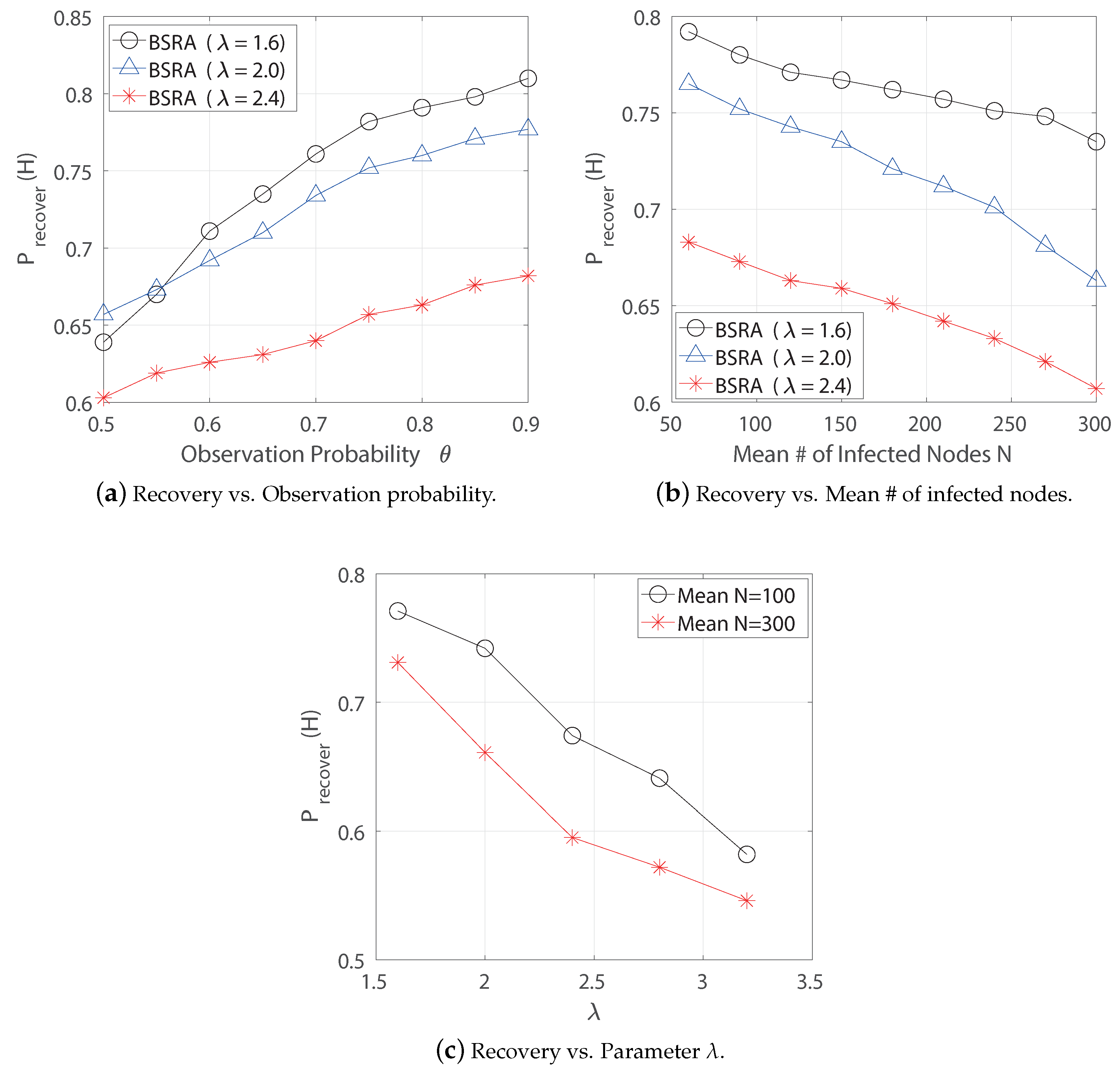
Next, the recovery performance of the BSRA is shown in Figure 5. For the simulation, the parameter is set to 2 for the source estimation. As the first result of the BSRA, the recovery probability is obtained by varying the observation probability in Figure 6a. In contrast to the result of the NBRA (), the overall recovery probability increases as the observation probability increases. This is because, when a partial snapshot is given, the BSRA first finds nodes that are estimated to be sources in the entire infection graph. The diffusion probability is then compared based on this to find hidden infections. It is known [22] that the performance of estimating such sources is better when the number of observed nodes is large. In addition, it can be verified that the recovery performance is better when the parameter of the ER random graph is than in other cases. This is because, when , the underlying ER graph has a local tree structure, as shown in Figure 1, in which the proposed BFS tree-based algorithm works well. In Figure 6b, the recovery probability is presented by varying the mean number of infected nodes N. The result shows that the probability decreases as N increases owing to the fact that the source estimation accuracy decreases when the number of infected nodes becomes large in general [22]. The result also shows that the probability of recovery when is the largest among the three values () because of the local tree structure of the underlying graph. In Figure 6c, the result is obtained by varying the parameter from 1.6 to 3.2 for the mean number of infected nodes as 100 and 300, respectively. For both cases, the recovery probability decreases as increases from 1.6 for both cases. Furthermore, owing to the better source estimation result when a small number of infected nodes occurs in the graph, the overall recovery probability when is better than that when
6.1.3. Performance Comparison
To compare the performance of the recovery probability in Equation (1), four algorithms are considered: (i) NBRA(), (ii) BSRA, (iii) Steiner, and (iv) NETFill. In the evaluation, each algorithm propagated the infection until 200 nodes in the graph on average. For NBRA(), and is set for NetFill. For Steiner, the min-Steiner tree method in Reference [6] is used. With this algorithm, however, a single source is considered; thus, the min-dist is used as the source estimation step, which selects the “centroid” node with the minimum weight in Reference [6] to estimate multiple sources as ranked values. The min-Steiner tree is then applied for the top-three sources separately and obtains the results. Finally, the recovery probabilities for each algorithm are listed in Table 2 and Table 3 as the observation probability and the parameter , respectively. As a result, in Table 2, the recovery probability of BSRA is higher than that of NETFILL, which is designed for the SI-diffusion model. Further, the results show that the performance of NBRA() is not inferior to that of the other three approaches, despite using only the local neighbor infection state information. Finally, in Table 3, it is concluded that the overall recovery performance decreases as the parameter increases. However, BSRA performs well compared to the other methods.
7. Conclusions
In this paper, a cascade infection-recovery problem was studied through a partial observation over an ER random graph. To do so, two algorithms, (i) a neighbor-based recovery algorithm and (ii) BFS tree source-based recovery algorithm, have been proposed. In the first algorithm, the number of infected neighbors were counted for candidate hidden cascade nodes and the possibility of infection was computed from the neighbors. In the second algorithm, the cascade sources were estimated, and the infection probability was computed from the BFS tree approximation for the underlying ER random graph with respect to the sources. Due to computational complexity, the approximated probability is considered for comparing the pre-defined criteria for recovery. The results show that the neighbor-based algorithm recovers the hidden cascade infection well and is not significantly affected by the average degree of the ER random graph. Furthermore, the BFS source-based method works well on a local tree-like structure.
8. Limitations and Future Works
The main advantage of the neighbor-based algorithm is that it does not require infection information spread over the entire graph to estimate whether a node is truly infected. In addition, it was confirmed that the results are not bad compared to the recovery performance of the other algorithms. In the case of the source-based algorithm, the recovery performance outperforms the comparison algorithms by adopting the OJC, which is known to be an extremely good technique for finding cascade sources in the ER graph. However, owing to mathematical intractability, the theoretical result obtained for the neighbor-based algorithm has a limitation in computing the probability of considering an actual uninfected node as infected. Furthermore, for the source-based method, when there is a loop in the graph, it is difficult to accurately calculate the infection probability from the source. Hence, a study on how to overcome these two limitations will be area of future work.
Funding
This work was supported by the National Research Foundation of Korea (NRF) grant funded by the Korea government (MSIT) (No. 2019R1G1A1099466).
Conflicts of Interest
The author declares no conflict of interest.
Appendix A. Proof of Theorem 1
From the algorithm NBRA(), we have the detection probability of the hidden infected node by
Let , and let , where . Then, we see that, if A′ is satisfied, then A is also satisfied, i.e., . Using this fact and by denoting , we have
where the last step is from the fact that Then, we have that, if satisfies the condition , then , which implies . This completes the proof.
References
- Woo, J.; Ok, J.; Yi, Y. Iterative learning of graph connectivity from partially-observed cascade samples. In Proceedings of the Twenty-First International Symposium on Theory, Algorithmic Foundations, and Protocol Design for Mobile Networks and Mobile Computing (Mobihoc ’20), online. 11–14 October 2020. [Google Scholar]
- Liu, Y.; Bao, Z.; Zhang, Z.; Tang, D.; Xiong, F. Information cascades prediction with attention neural network. Hum. Cent. Comput. Inf. Sci. 2020, 10, 13. [Google Scholar] [CrossRef]
- Feng, X.; Zhao, Q.; Liu, Z. Prediction of information cascades via content and structure proximity preserved graph level embedding. Inf. Sci. 2021, 560, 424–440. [Google Scholar] [CrossRef]
- Netrapalli, P.; Sanghavi, S. Finding the Graph of Epidemic Cascades. ACM SIGMETRICS Perform. Eval. Rev. 2012, 40, 211–222. [Google Scholar] [CrossRef]
- Sundareisan, S.; Vreeken, J.; Prakash, B.A. Hidden Hazards: Finding Missing Nodes in Large Graph Epidemics. In Proceedings of the 2015 SIAM International Conference on Data Mining (SDM), Vancouver, BC, Canada, 30 April–2 May 2015. [Google Scholar]
- Xiao, H.; Aslay, C.; Gionis, A. Robust Cascade Reconstruction by Steiner Tree Sampling. In Proceedings of the IEEE International Conference on Data Mining (ICDM), Singapore, 17–20 November 2017. [Google Scholar]
- Xiao, H.; Rozenshtein, P.; Tatti, N.; Gionis, A. Reconstructing a cascade from temporal observations. In Proceedings of the 2018 SIAM International Conference on Data Mining (SDM), San Diego, CA, USA, 3–5 May 2018. [Google Scholar]
- Wu, X.; Kumar, A.; Sheldon, D.; Zilberstein, S. Parameter Learning for Latent Network Diffusion. In Proceedings of the Twenty-Third International Joint Conference on Artificial Intelligence, Beijing, China, 3–9 August 2013. [Google Scholar]
- He, X.; Liu, Y. Not Enough Data? Joint Inferring Multiple Diffusion Networks via Network Generation Priors. In Proceedings of the Tenth ACM International Conference on Web Search and Data Mining, Cambridge, UK, 6–10 February 2017. [Google Scholar]
- Choi, J. Identification of Individual Infection Over Networks With Limit Observation: Random vs. Epidemic? IEEE Access 2021, 9, 74234–74245. [Google Scholar] [CrossRef]
- Huang, Y.; Feamster, N.; Teixeira, R. Practical Issues with Using Network Tomography for Fault Diagnosis. ACM SIGCOMM Comp. Commun. Rev. 2008, 38, 53–58. [Google Scholar] [CrossRef]
- Tosic, T.; Thomos, N.; Frossard, P. Distributed sensor failure detection in sensor networks. Signal Process. 2013, 93, 399–410. [Google Scholar] [CrossRef] [Green Version]
- Nasiri, M.; Mobayen, S.; Zhu, Q. Super-Twisting Sliding Mode Control for Gearless PMSG-Based Wind Turbine. Complexity 2019, 2019, 6141607. [Google Scholar] [CrossRef]
- Jafari, M.; Mobayen, S. Second-order sliding set design for a class of uncertain nonlinear systems with disturbances: An LMI approach. Math. Comput. Simul. 2019, 156, 110–125. [Google Scholar] [CrossRef]
- Abadie, J.P.; Horel, T. Inferring Graphs from Cascades: A Sparse Recovery Framework. In Proceedings of the 32nd International Conference on Machine Learning, Lille, France, 7–9 July 2015. [Google Scholar]
- Abrahao, B.; Chierichetti, F.; Kleinberg, R.; Panconesi, A. Trace Complexity of Network Inference. In Proceedings of the 19th ACM SIGKDD International Conference on Knowledge Discovery and Data Mining, Chicago, IL, USA, 11–14 August 2013. [Google Scholar]
- He, X.; Xu, K.; Kempe, D.; Liu, Y. Learning Influence Functions from Incomplete Observations. In Proceedings of the Advances in Neural Information Processing Systems 29 (NIPS 2016), Barcelon, Spain, 5–10 December 2016. [Google Scholar]
- Rozenshtein, P.; Gionis, A.; Prakash, B.; Vreeken, J. Reconstructing an Epidemic Over Time. In Proceedings of the 22nd ACM SIGKDD International Conference on Knowledge Discovery and Data Mining, San Francisco, CA, USA, 13–17 August 2016. [Google Scholar]
- Gripon, V.; Rabbat, M. Reconstructing a Graph from Path Traces. In Proceedings of the 2013 IEEE International Symposium on Information Theory, Istanbul, Turkey, 7–12 July 2013. [Google Scholar]
- Amin, K.; Heidari, H.; Kearns, M. Learning from Contagion (Without Timestamps). In Proceedings of the 31st International Conference on Machine Learning, Beijing, China, 21–26 June 2014. [Google Scholar]
- Zhu, K.; Ying, L. Information source detection in networks: Possibility and impossibility result. In Proceedings of the IEEE INFOCOM 2016—The 35th Annual IEEE International Conference on Computer Communications, San Francisco, CA, USA, 10–14 April 2017. [Google Scholar]
- Zhu, K.; Chen, Z.; Ying, L. Catch’Em All: Locating Multiple Diffusion Sources in Networks with Partial Observations. In Proceedings of the Thirty-First AAAI Conference on Artificial Intelligence (AAAI-17), San Francisco, CA, USA, 4–9 February 2017. [Google Scholar]
- Zhu, K.; Chen, Z.; Ying, L. Locating the contagion source in networks with partial timestamps. Data Min. Knowl. Discov. 2016, 30, 1217–1248. [Google Scholar] [CrossRef]
- Fanti, G.; Kairouz, P.; Oh, S.; Ramchandran, K.; Viswanath, P. Metadata-Conscious Anonymous Messaging. In Proceedings of the 33rd International Conference on Machine Learning, New York, NY, USA, 20–22 June 2016. [Google Scholar]
- Liu, X.; Fu, L.; Jiang, B.; Lin, X.; Wang, X. Information Source Detection with Limited Time Knowledge. In Proceedings of the Twentieth ACM International Symposium on Mobile Ad Hoc Networking and Computing, Catania, Italy, 2–5 July 2019. [Google Scholar]
- Tang, W.; Ji, F.; Tay, W. Estimating Infection Sources in Networks Using Partial Timestamps. IEEE Trans. Inf. Forensics Secur. 2018, 13, 3035–3049. [Google Scholar] [CrossRef] [Green Version]
- Kumar, A.; Borkar, V.S.; Karamchandani, N. Temporally Agnostic Rumor-Source Detection. IEEE Trans. Signal Inf. Process. Netw. 2017, 3, 316–329. [Google Scholar] [CrossRef]
- Hartigan, J.A.; Wong, M.A. Algorithm as 136: A k-means clustering algorithm. J. R. Stat. Soc. Ser. C Appl. Stat. 1979, 28, 100–108. [Google Scholar] [CrossRef]
Figure 1.
Illustration example of the ER random graph for 500 nodes. (We set the average degree as (left), (middle), and (right). The figure shows that, for a given number of nodes n, the ER random graph has local tree structures if the average number of degrees .).
Figure 1.
Illustration example of the ER random graph for 500 nodes. (We set the average degree as (left), (middle), and (right). The figure shows that, for a given number of nodes n, the ER random graph has local tree structures if the average number of degrees .).

Figure 2.
A simple observed graph with infection probabilities used in Example 1.

Figure 3.
Example of Step 1 (Candidate Infection Path Selection): In the example, the underlying ER random graph G is generated as two disconnected sub-graphs (leftmost). If there is only one cascade source, the cascade occurs only in one connected sub-graph, denoted as (second from the left). Based on this, the algorithm first constructs the BFS tree (third from the left). It then selects the set of candidate neighbors for node v. In this example, the distance from the estimated source to v is . Therefore, two nodes (labelled as 1 and 2) are chosen as candidate neighbor nodes because their distance from is 1. Node 2 is already a neighbor in , and node 1 is finally selected as the candidate neighbor and connects an edge to the node v (rightmost). This is referred to as a reconstructed graph , and the algorithm selects the candidate infection paths including the candidate neighbor node (yellow arrows).
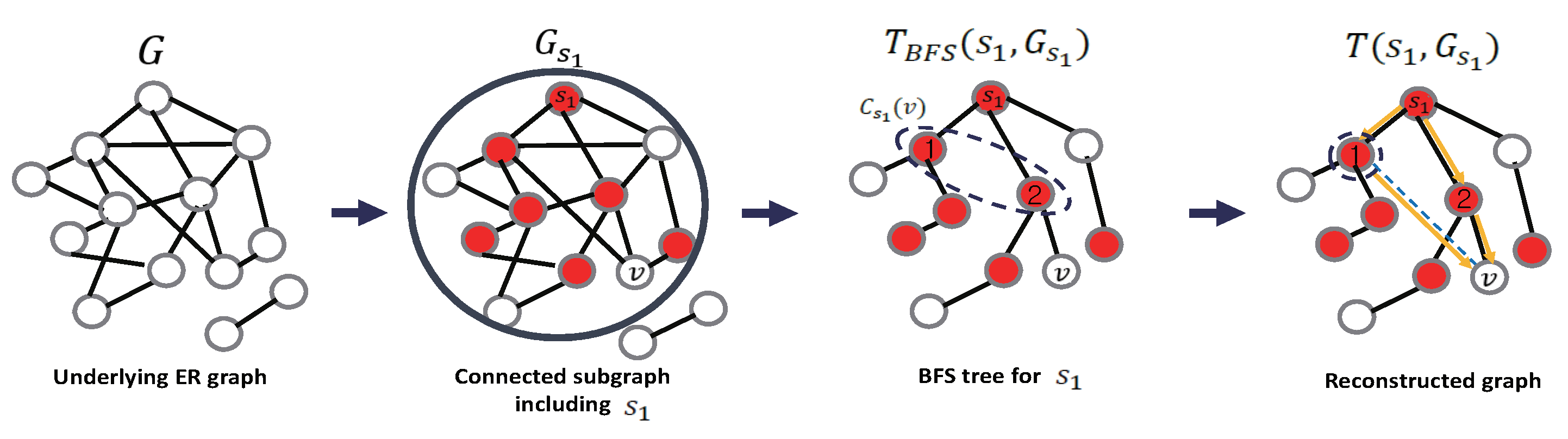
Figure 4.
Illustration example of the Algorithm BSRA for . The BSRA first estimates the sources for a given then it makes m different BFS trees with respect to each source . Next, for each node , the BSRA reconstructs graph for each (see Figure 3) and computes the infection probability using . After computing the diffusion probability from the sources, it finally recovers the hidden infected node based on the criteria, as in the right figure.
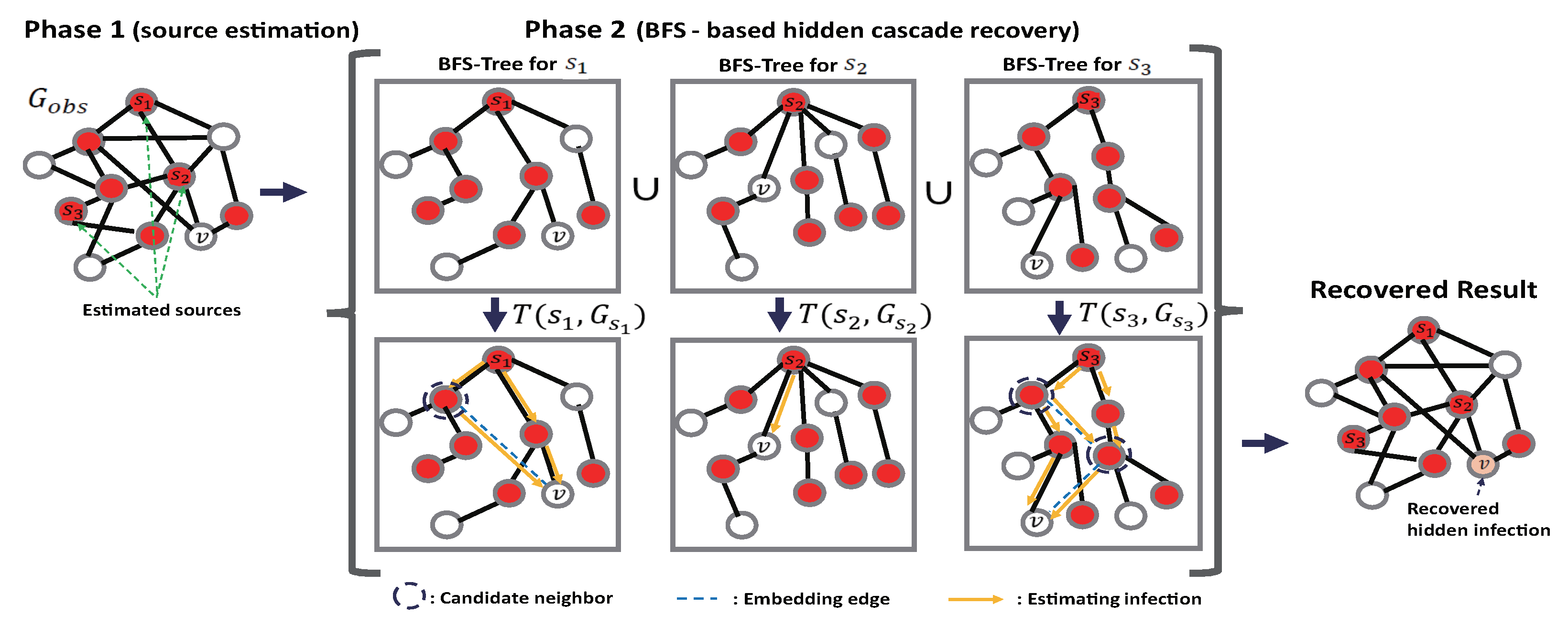
Figure 5.
Recovery probabilities of NBRA() for . ((a) Recovery as the observation probability varies from 0.5 to 0.9. (b) Recovery by varying the mean number of infected nodes from 60 to 300. (c) Recovery by varying the parameter from 0.1 to 0.9. Here, N indicates the mean number of infected nodes).
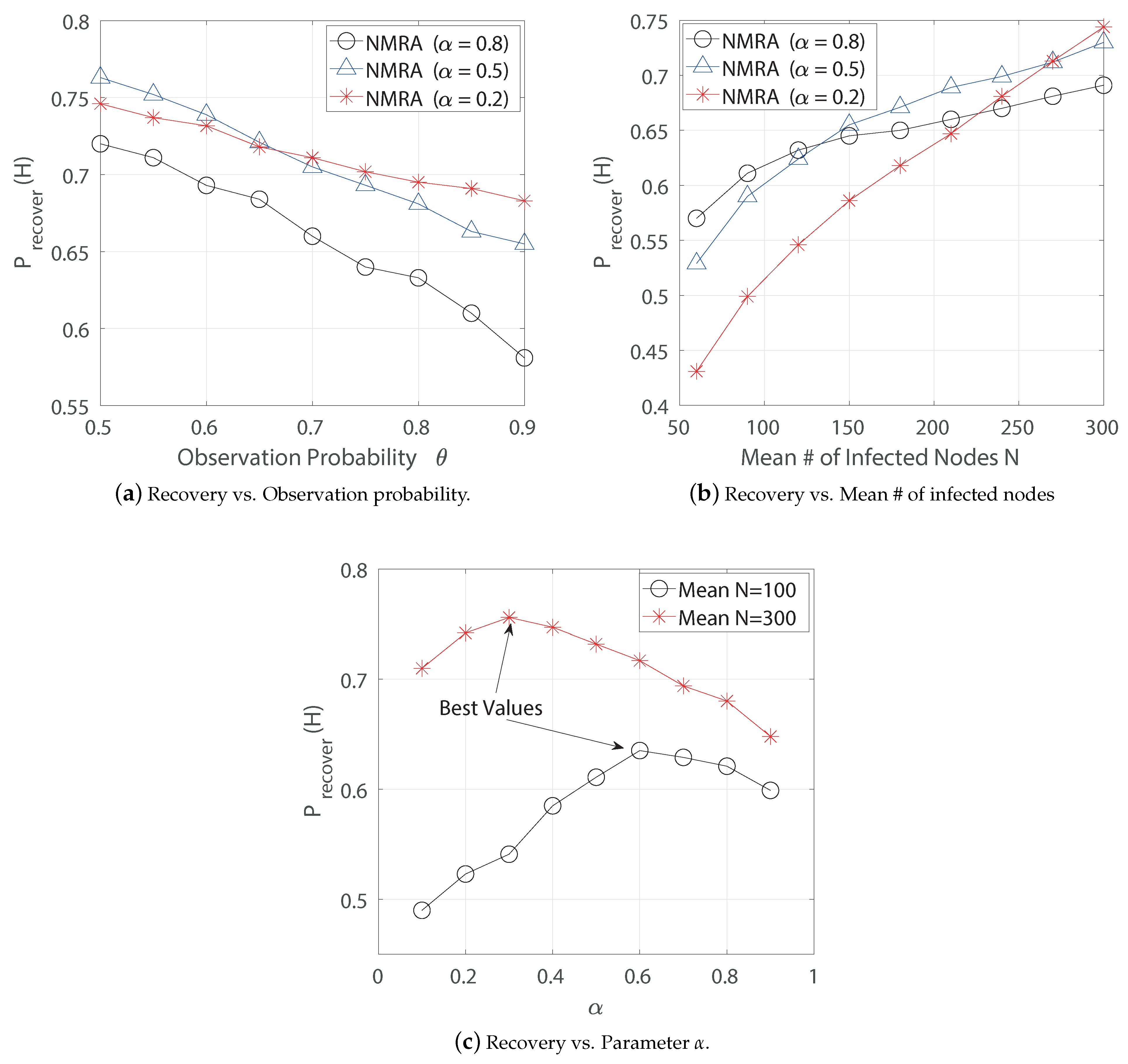
Figure 6.
Recovery probabilities of NBRA() for and . ((a) Recovery as the observation probability varies from 0.5 to 0.9. (b) Recovery by varying the mean number of infected nodes from 60 to 300. (c) Recovery as varying the parameter from 1.6 to 3.2).
Figure 6.
Recovery probabilities of NBRA() for and . ((a) Recovery as the observation probability varies from 0.5 to 0.9. (b) Recovery by varying the mean number of infected nodes from 60 to 300. (c) Recovery as varying the parameter from 1.6 to 3.2).

Table 1.
Summary of notations.
| Notation | Explanation |
|---|---|
| ER random graph with two parameters n and p | |
| Average degree of a node in | |
| Infection probability from node u to v | |
| Infection probability over edge e | |
| Infection reporting probability for node v | |
| Infection probability vector for all edges | |
| Infection-reporting probability vector for all nodes | |
| , S | (True) Cascade source, Set of cascade sources |
| Set of observed (reported) infected nodes | |
| Observed cascade snapshot at time t | |
| m | Number of cascade sources |
| , | Estimated (i-th) cascade source, Estimated set of cascade sources |
| Infection status of a node v | |
| Estimator of | |
| recovery probability of | |
| Set of hidden (not reported)-infected nodes | |
| Estimated recovering set | |
| Set of (reported) infected neighbors of a node v | |
| Minimum diffusion probability among for all | |
| Infection eccentricity of node set S over | |
| Selection threshold | |
| W | Set of nodes with more than observed infected neighbors |
| Union of W and | |
| Induced graph (connected subgraph of ) from | |
| Connected sub-graph of G including | |
| BFS tree over w.r.t. | |
| Candidate neighbor (infected) set of v in | |
| Reconstructed graph from | |
| Union of and | |
| T | Union of reconstructed graphs |
| Path between node v and source node in | |
| Pre-defined threshold for determining the infection of node v | |
| () | Maximum (minimum) infection probability over T from S |
Table 2.
Recovery probabilities of four algorithms: (i) NBRA(), (ii) BSRA, (iii) Steiner, and (iv) NETFILL as varying the observation probability .
Table 2.
Recovery probabilities of four algorithms: (i) NBRA(), (ii) BSRA, (iii) Steiner, and (iv) NETFILL as varying the observation probability .
| NBRA() | BSRA | Steiner | NETFILL | |
|---|---|---|---|---|
| 0.69 | 0.65 | 0.71 | 0.61 | |
| 0.68 | 0.67 | 0.69 | 0.57 | |
| 0.65 | 0.72 | 0.67 | 0.55 | |
| 0.62 | 0.75 | 0.64 | 0.53 | |
| 0.61 | 0.77 | 0.63 | 0.54 |
Table 3.
Recovery probabilities of four algorithms: (i) NBRA(), (ii) BSRA, (iii) Steiner, and (iv) NETFILL as varying the ER graph parameter .
Table 3.
Recovery probabilities of four algorithms: (i) NBRA(), (ii) BSRA, (iii) Steiner, and (iv) NETFILL as varying the ER graph parameter .
| NBRA() | BSRA | Steiner | NETFILL | |
|---|---|---|---|---|
| 0.59 | 0.73 | 0.69 | 0.64 | |
| 0.62 | 0.71 | 0.67 | 0.56 | |
| 0.65 | 0.67 | 0.63 | 0.51 | |
| 0.64 | 0.63 | 0.59 | 0.48 | |
| 0.65 | 0.58 | 0.55 | 0.44 |
Publisher’s Note: MDPI stays neutral with regard to jurisdictional claims in published maps and institutional affiliations. |
© 2021 by the author. Licensee MDPI, Basel, Switzerland. This article is an open access article distributed under the terms and conditions of the Creative Commons Attribution (CC BY) license (https://creativecommons.org/licenses/by/4.0/).
Share and Cite
MDPI and ACS Style
Choi, J. Inferring the Hidden Cascade Infection over Erdös-Rényi (ER) Random Graph. Electronics 2021, 10, 1894. https://doi.org/10.3390/electronics10161894
AMA Style
Choi J. Inferring the Hidden Cascade Infection over Erdös-Rényi (ER) Random Graph. Electronics. 2021; 10(16):1894. https://doi.org/10.3390/electronics10161894
Chicago/Turabian StyleChoi, Jaeyoung. 2021. "Inferring the Hidden Cascade Infection over Erdös-Rényi (ER) Random Graph" Electronics 10, no. 16: 1894. https://doi.org/10.3390/electronics10161894
Note that from the first issue of 2016, this journal uses article numbers instead of page numbers. See further details here.