Abstract
The conventional AC microgrid power regulation method is achieved using dual undulations of the grid-side voltage and frequency, whose complex variables and processes make the system less efficient and stable. For this problem, this paper proposes a novel two-hierarchical small signal model stability analysis for islanded AC microgrid systems with a designed power regulation algorithm under the constant frequency, mainly aimed at the continual switching microgrids, and considers the future expansion. MATLAB/Simulink simulations and experiments are conducted to validate the feasibility. It is found that there is a strong consistency between the stability of primary and overall systems, and that two key parameters affect the stability properties. Discussing the mutual influence of various parameters, is positively correlated with control intensity and determines the proportion of reactive power distribution in each power generation. Contrasting with the previous complex processes, the unique points of this method are the simplicity of calculation, parameter induction, response testability, strong operability, and system extensibility. The conclusion is that this constant frequency power control is simple, feasible, and stable under several specified conditions.
1. Introduction
Microgrid is an advanced method for integrating distributed energy sources (DERs), converters, energy storage, and loads [1,2]. Distributed energy is widely used to generate electricity from wind, solar photovoltaic, hydroelectric, or biomass energy, taking into account the impact on the environment. However, owing to the uncertainty of the production capacity of these renewable energy sources, how to effectively control and reasonably distribute the power of the microgrid has become a major problem [3].
The most widely used method is the droop method, which has certain reliability and flexibility [4,5]. However, owing to admittance mismatch in droop control [3,4,5,6], the reactive power distribution effect is not ideal. A method to improve the accuracy of reactive power tracking is proposed in [7]. Other methods of smoothing power changes for balance are presented in [8,9], at the expense of frequency stability. In a general design, ignoring some constraints can degrade the performance of the system [10]. However, these limitations may lead to excessive or frequent load fluctuations, leading to overload problems, which can be solved using some non-communication methods [11,12]. Another commonly used method to solve the mismatch problem is virtual impedance estimation [13,14,15,16,17,18]. Some excellent FM virtual impedance methods are used in [19,20,21]. The introduced voltage derivative is effective, but a reactive power error exists [22,23,24]. The overload problem in droop control can be reduced by limiting the current, but the fixed power range will interfere with the voltage loop [25,26]. The attempted constant frequency droop method will make the power calculation inaccurate [27,28,29,30]. This shows that it is not feasible to simplify the calculation by only considering the constant frequency in droop control. Using the load reduction idea in [31], a better rational power distribution droop method is proposed. However, when the system is not scalable, the frequency cannot be recovered. Excessive sag will lead to excessive voltage and frequency deviation, affecting voltage quality and stability. The reverse droop method can avoid these problems and has the advantages of fast response, small current ripple, good stability, good performance, and so on. The main disadvantage of the reverse droop method is that the system response speed is fast, which leads to a surge in inverter cost.
Another approach is master-slave control. Its advantage is that it can be used as the main controller to fix the system voltage and frequency. Nevertheless, the control feedback cannot limit the energy entering the region [32]. There is a method of enhancing cooperative control that can be improved, but it is not as effective as [33]. Energy storage devices are also used in this method to attempt constant frequencies, which in turn exacerbates the overload problem [34,35].
Different from droop control, adaptive control is one of the popular trends in recent years. It introduces precise power allocation in communication [14,36,37,38,39]. Consistent control has the advantages of good robustness and low cost. However, it always has the problem of time lag [40,41,42,43,44,45]. In two papers [46,47], a comparison was made between various mainstream methods and special methods.
At present, the commonly used constant frequency power regulation technologies include the V-P control method under constant frequency [19,20,21], droop [27,28,29,30], master-slave [34,35], and so on. However, most of them cause overload, precision, or complex communication problems. At present, there is no suitable power regulation scheme to solve the problems of frequency conversion, large load, and power accuracy. Thus, it is necessary to have equations derived by the system. In this paper, a voltage-dependent power regulation algorithm is proposed for fixed-frequency AC microgrids. The algorithm supports equal distribution of active power and better distribution of reactive power. The coefficient is specifically designed for AC microgrids with scalable switching topologies.
In other papers [19,20,48], Matlab/Simulink-based real-time models have been built for the constant frequency operated islanded microgrid. However, detailed analysis on stability and experimental validation has not been carried out yet. Such gaps will be filled. The main contributions of this paper can be summarized as below:
- A low-dependence power regulation algorithm is proposed with designed coefficients for AC microgrids, which is used to fast track reference power with a fixed frequency. The proposed algorithm allows power to be properly shared by individual power generation, even under large load variations.
- Concise coefficients’ definition in the proposed algorithm influences the inherent feature and tracking effect. These coefficients are involved in transfer function formulation, used to calculate the boundary of the valid parameter region.
- Transfer functions of the proposed algorithm for primary and secondary levels of the AC microgrid system are derived in detail. Its characteristics, stability proof, and response behavior are also discussed. The size of the AC system can be arbitrarily expanded to meet relevant requirements, which is very helpful for future development.
The remained of this paper is arranged as below. Section 2 is the main control strategy. Primary and secondary level small signal models are proposed in Section 3 and Section 4. Section 5 studies system dynamics characteristics. Simulations, laboratory experiments and discussions are provided in Section 6. The conclusion is summarized in Section 7.
2. Control Strategy
2.1. Power Reference Calculation
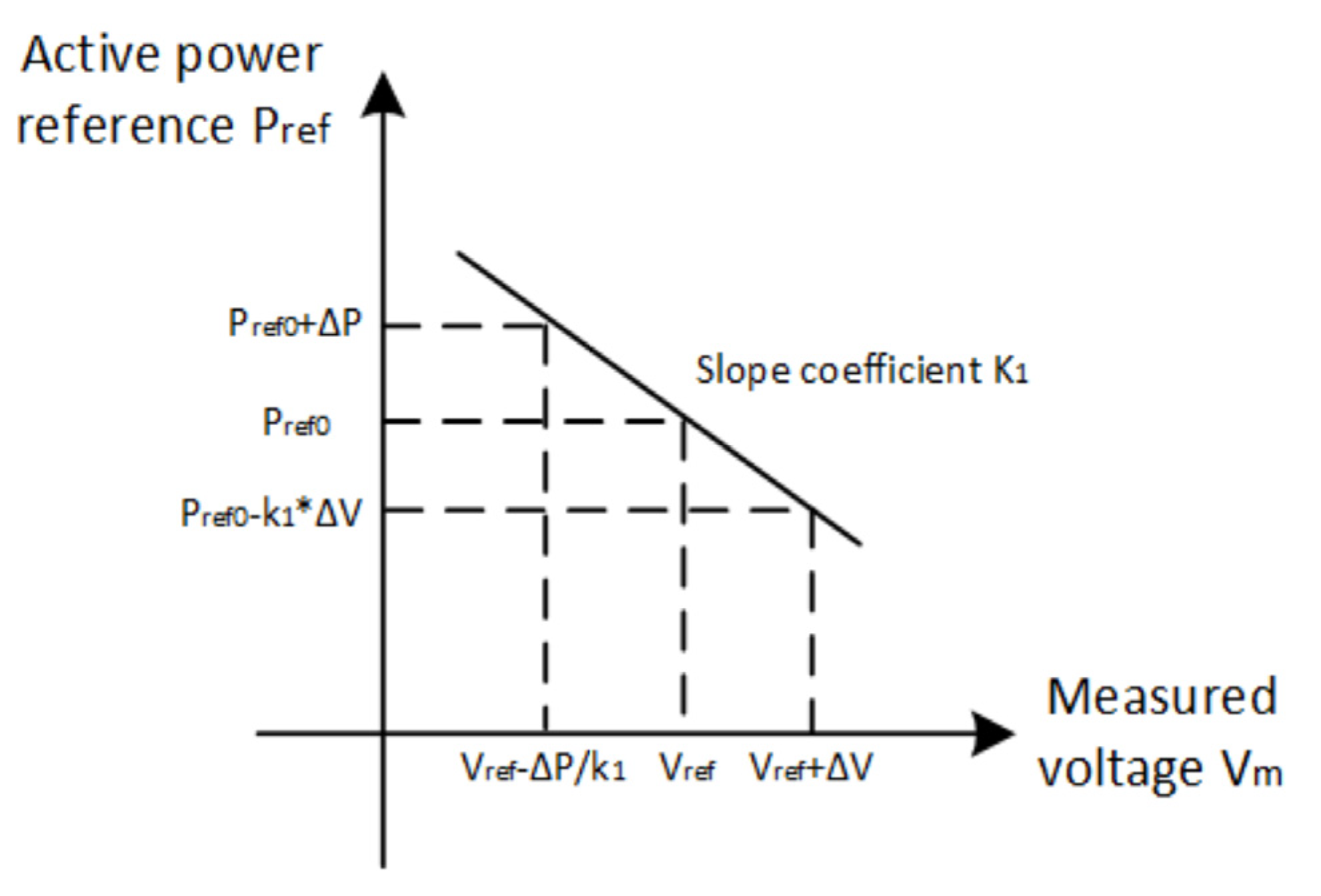
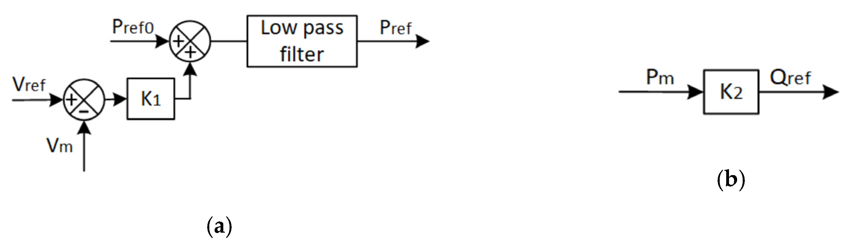
In each inverter, the control algorithm for power regulation is specified in Figure 1. In the voltage against active power in the constant frequency method, active power is managed by voltage variation only, when the frequency is kept at 50 Hz. The active power reference is generated by adding voltage change into the nominal reference active power with a coefficient . Figure 2 indicates that the reference reactive power in a grid-supporting generator is a directly certain percentage of the measured active power. Reactive power in grid-supporting generators tracks the given percentage, while the rest of the reactive power is produced by grid forming generators. The grid forming generator senses the total demand and the portion that is already provided. The two generators co-operate to meet all the reactive power requirements of the load. The microgrid system consists of two parts; the DC side nominal voltage is 800 V, while the load side AC nominal voltage is 415 V. Thus, voltage and current do not deviate too much near these power levels.
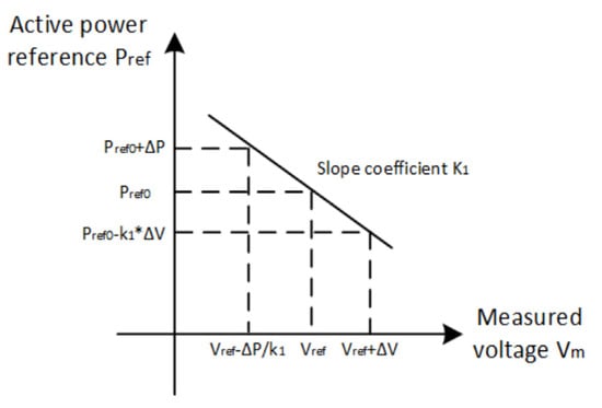
Figure 1.
V-P control algorithm line chart.
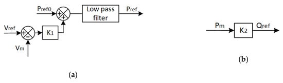
Figure 2.
Power reference calculation. (a)active power reference calculation, (b) reactive power reference calculation.
The active power reference for this control law is (1).
Laplace transformed low pass filter is in the form of (2).
As the operating point is around nominal reference active power, the small deviations around this point build the small-signal model, for stability and coefficients analysis.
From (1), active power is moved to the left side and voltage to the right side for calculation.
The fluctuation relationship in active power and voltage is provided in (3).
Putting (2) into (3), when , with no filter for voltage measurement, (4) is obtained, which is rearranged as (5).
Using inverse Laplace transformation back to the time domain, we obtain (6), then organize (6) into the standard ordinary differential equation form (7).
(7) is the most important basic formula used in this control algorithm.
2.2. Control Strategy
The basic control strategy in the local loop is to fix voltage and regulate the current control loop. When reference power is generated, corresponding reference voltage and current are formed. These references are decoupled into d-q frame. Each branch voltage tracks the given reference, while current tracks the varying reference, so that the power level could be reached. The instantaneous load current, voltage, and angle are measured by the phase lock loop after the LC filter, later to be sent into controllers for feedback regulation.
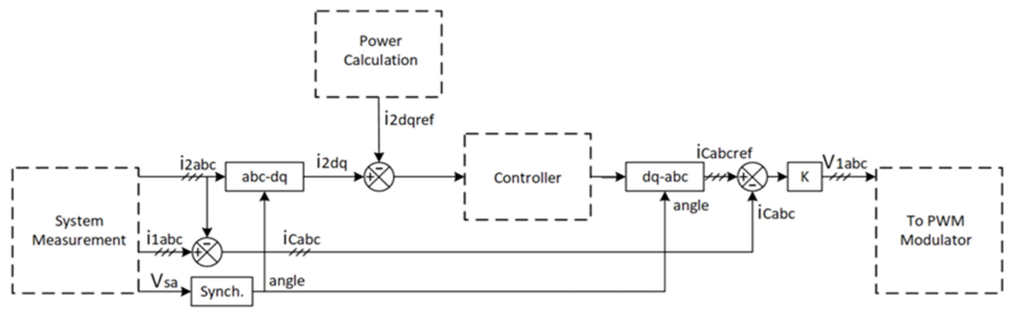
In the controller, the configuration is provided in Figure 3. The measured voltage and current are converted into the d-q frame, and synchronized with the grid value. They are subtracted from the calculated reference value and sent to the controller. After a precise magnification, they are finally sent to the gating signal of the distributed generation inverter. As a result, the output of the inverter follows the reference after the LC filter.
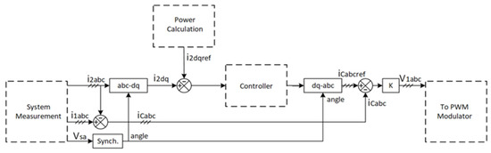
Figure 3.
Controller configuration.
In Figure 3, and are the a-b-c frame current and voltage from the inverter side, is the a-b-c frame current from the load side, is the capacitor current from the LCL filter, is the converted d-q frame current from the load side, and and are the nominal voltage and angle of the main bus.
The reference active and reactive power in Figure 3 is calculated in Figure 2 using the proposed voltage against active power algorithm. Then, this reference is decoupled into voltage and current reference , and sent to the control system for tracking. The grid voltage, inverter side current, and load side current are collected and converted. The PLL processes the voltage signal to obtain the frequency and angle for synchronization. Current signals are converted from a-b-c frame into d-q frame for regulation. The d-q frame signal is sent to controller to track and using the proportional integral controller. The generated control input signal is converted back into a-b-c frame and multiplied by a certain gain to become a voltage control input signal, which goes to the PWM for the inverter.
In this system, all kinds of controllers can be applied to implement this active power tracking. The aim is to follow the reference current at the desired voltage level, so the reference power can be reached.
The conventional linear state feedback controllers such as pole-placement control might be used. However, the workload of the early calculation is increased because of the internal dynamics computation in advance, using system identification. The common PID controller is also suitable here because of its advantages of simple formulation, easy adjustment, and flexibility.
Another choice is the optimal controller, such as linear quadratic regulator or model predictive control. Cost functions can be designed and compared to the target system in future work. Energy-based cost functions are good choices to be considered. Later work will be done on this optimization.
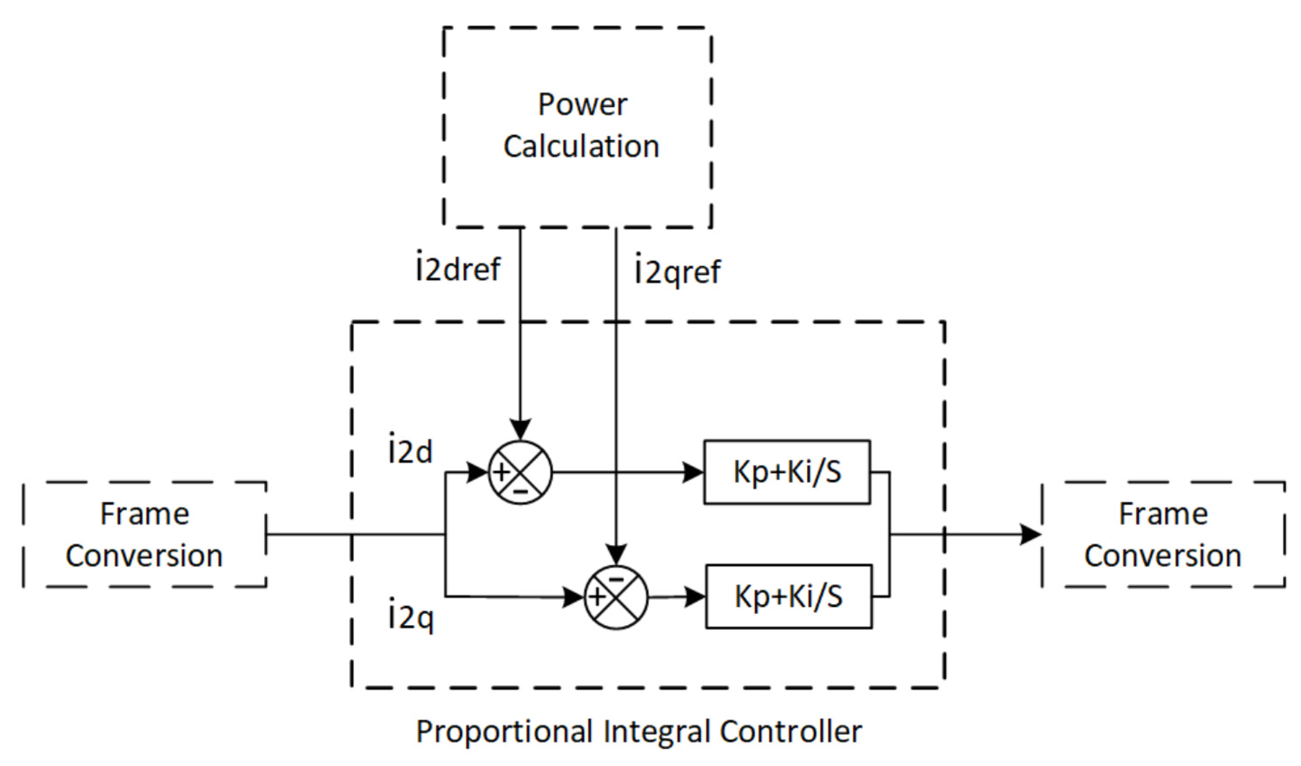
At an early stage, effective and flexible controllers are preferred. Now, we adopt a proportional integral (PI) controller in the synchronous rotating reference frame shown in Figure 4. Figure 4 is a detailed enlarged version of the controller module in Figure 3. The ‘frame conversion’ blocks on the left and right side of Figure 4 are the same a-b-c frame and d-q frame interconversions from Figure 3. This controller has less computation and can be tuned easily.
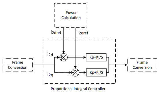
Figure 4.
PI controller adopted in the system.
3. Primary Level Small-Signal Model
The primary control feedback loop is given in Figure 3 in each generator, used to keep the desired voltage and track reference power.
3.1. General Voltage and Angle Knowledge
Firstly, voltage amplitude and angle are measured and checked in a synchronous rotating frame [49,50,51].
Voltage can be split into and in the d-q frame in (8), with the angle relationship in (9). This angle is shown in Figure 3, found by PLL.
Suppose a, b, c, and d are generated as (10) [49,50].
Instantaneous deviation relationships in voltage and angle around equilibrium points are given in (11) and (12).
These two equations hold for their partial derivatives in (13) and (14) as well.
Now, is found to cancel the term, then (15) is obtained.
Further, is calculated to cancel the term, so (16) is obtained.
Angle deviation is the integral of frequency in the s-domain, which is (17).
In the time domain, the relationship would be (18).
This system is under the condition of constant frequency so that the frequency deviation could be treated as zero, resulting in (19).
Thus, the term in (15) and (16) could be ignored in this system. Equations (15) and (16) now give voltage decoupling under constant frequency in the system. The frequency output from PLL and synchronization sections is constant in system sampling, control calculation, control input, and other parts. Any new access to the power generations or load modules will lock the frequency from the signal acquisition until the output parts. This ensures that the frequency of the system is fixed at about 50 Hz, and there is no phase shift in the three-phase circuit.
3.2. Primary Loop with Power Control Algorithm
Involving control coefficients, general Equation (12) is substituted into the reference calculation algorithm (7) to form (20).
Equation (20) gives voltage and active power relations.
Equation (20) is substituted into (15) and (16) to replace the term and obtain the matchup between power and decoupled voltage directly in (21) and (22).
Equations (21) and (22) are combined in matrix form. We have and as individual inverter dynamic states and power variance and regarded as control input in (23).
Equation (23) is the derived system model for individual inverter, where system matrices corresponding to states and input are and for the inverter in (24) and (25).
Open-loop stability feature is used to check matrix and the input coefficient is . Obviously, reactive power is not included in this control loop owing to the corresponding whole zero column. Thus, reactive power tracking follows only the ratio reference in another manner.
In this system, active power reaches equal power-sharing when loads are switching on and off. Reactive power in grid-supporting generators tracks the given percentage, while the rest of the reactive power is produced by grid forming generators. This ensures the system meets power requirements from loads.
4. Secondary Level Small-Signal Model
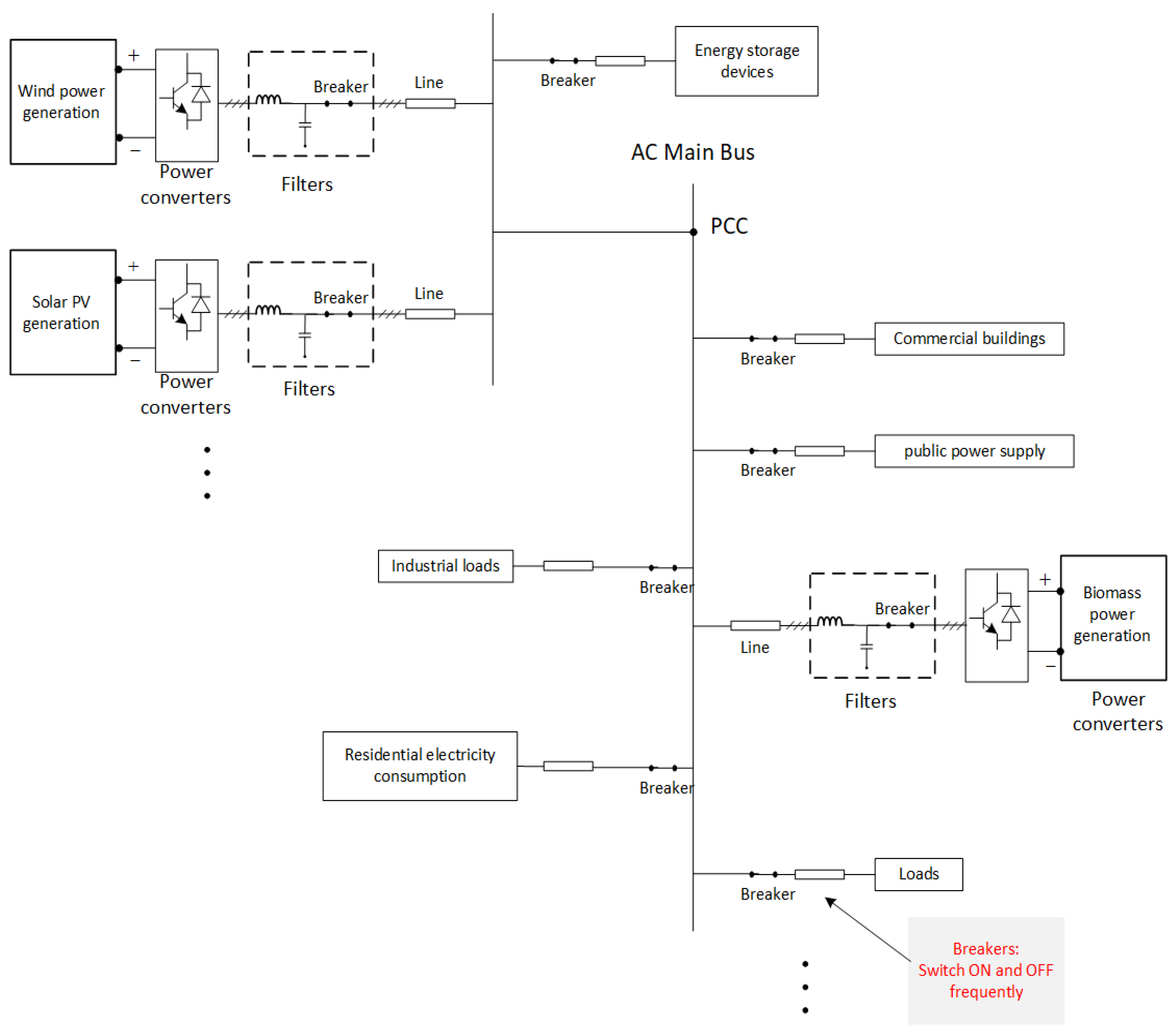
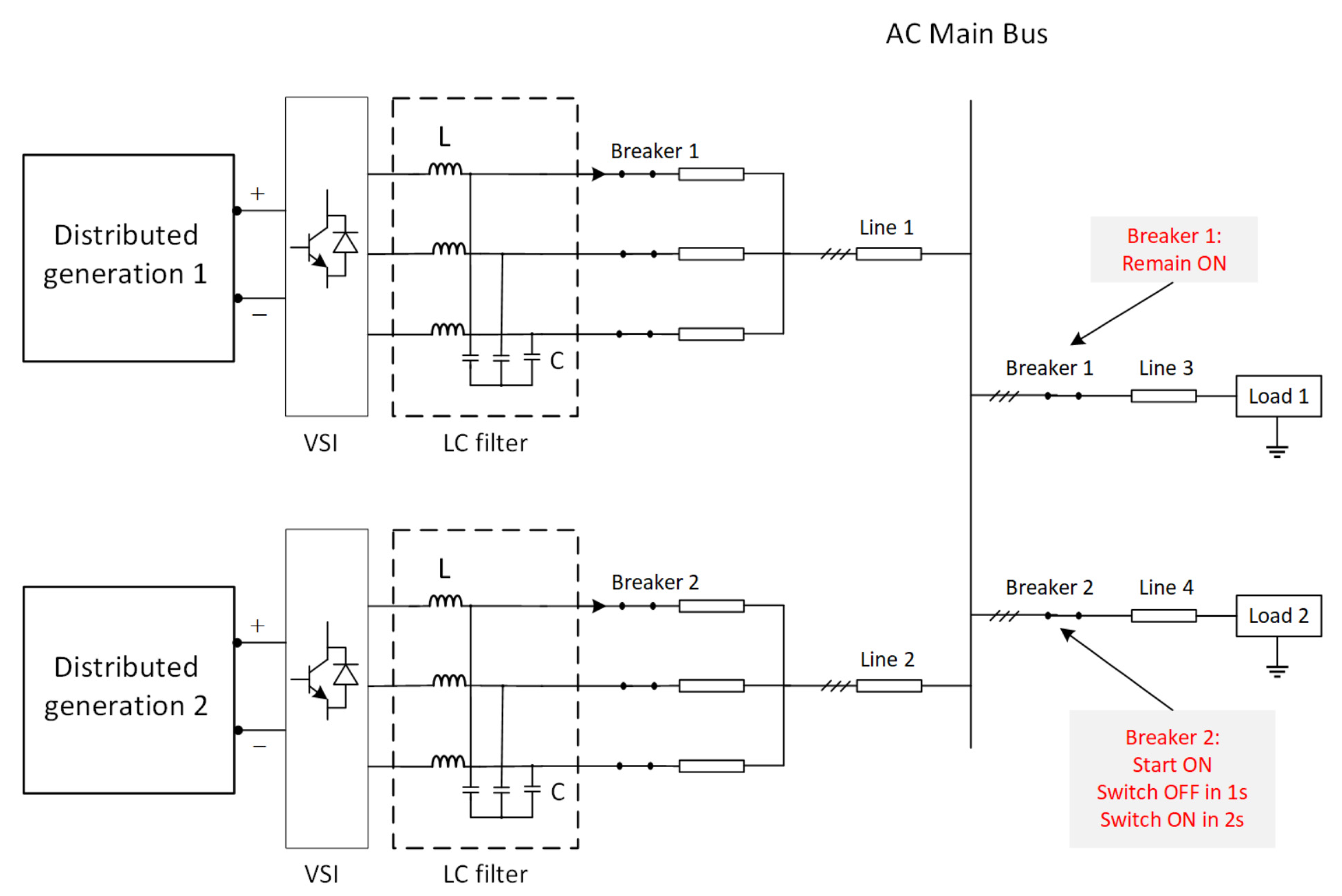
By connecting all inverters and load, the overall system is formed as shown in Figure 5. Distributed power generations can be wind power, solar power, hydroelectric power, or biological power generation. The overall system contains the generator side and the load side. On the generator side, several distributed generations are connected to inverters, filtered, and attached to the main AC bus. A switch between the filter and the main bus is for the synchronization check. On the load side, switch and load are linked in sequence. This system could be expanded into higher order, with more generations and loads, which could be switched on and off. Stability analysis is based on this structure.
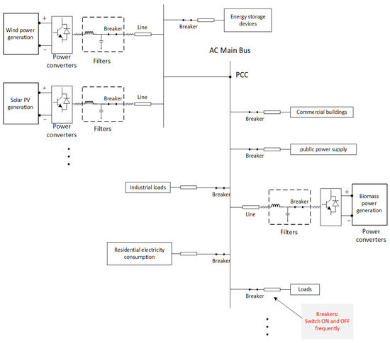
Figure 5.
AC microgrid system structure.
4.1. General Configuration Knowledge
Now, consider n inverter cases, with local loads connected. Current and voltage after inverters are given in (26).
To build the overall system, the nodal admittance matrix of the system must be worked out for all possible extended system structures in (27). As diagonal elements are nonnegative impedance, and non-diagonal ones are negative, as long as the impedance value is non-negative, the stability of the system will not be disrupted by excessive line resistance.
In the proposed small-signal model, we consider the deviations in grid voltage , current , and power , where matrices are given in (28)–(30).
For in the ith inverter (i = 1, 2, … n), we have each of them separated in (31)–(33).
System coefficients are . In these matrices, are the diagonal compound matrices with corresponding at the diagonal line for the inverter, where is from 1 to n. That is, . The specific matrix internal parameters are (34) and (35).
4.2. Secondary Loop with Control Coefficients
By augmenting (23) into a more concise form, we have (36).
From (26), we have the overall form in (37).
From active power and reactive power decomposition, we have (38).
In this system, the nominal voltage is fixed. In practice, we regulate the current to realize power control. Thus, is chosen to be the system dynamics in an overall system control loop.
Substituting (37) and (38) into (36), the current state-space model is formed in (39).
Reorganizing (39), the state space representation small-signal model of the current loop is (40).
5. System Dynamics Analysis
5.1. Secondary Level Stability Study
In (40), we check each matrix in to study its stability in the system. The overall system will be stable for poles having a negative real part.
Nodal admittance matrix is considered as a symmetric Hurwitz matrix, only used to find properties. Owing to the positive load resistance and line impedance, diagonal elements on matrix are positive, while off-diagonal elements are negative and smaller than diagonal elements. To say the least, if no load is connected to the inverter, the diagonal elements still include larger line impedance components. The imaginary part of each element in the matrix does not affect the stability property, so reactance is not a focus.
The matrix check is displayed in (41)–(44).
All Hurwitz determinants are positive for all k = 1, 2, 3, … n. It is obvious that all leading principal minors of matrix are positive, leading to the negative definite property. The determinant of is non-zero owing to non-zero diagonals, so is invertible. is also negative definite.
Moreover, matrix is symmetrical and negative definite. are diagonal matrices, as well as symmetric. Their properties depend on each diagonal element from each inverter i = 1, 2, 3…, n. The overall property depends on each element on the diagonal line, which is from each inverter.
That is, if each inverter is stable, the overall system will be stable under this configuration. The individual property is checked in Section 5.2.
5.2. Primary Level Stability Study
We study each diagonal element in to find poles in each inverter system.
is proven above to be negative definite. is the same when it is invertible. Now, check and .
Firstly, is always positive. Eigenvalues of and are shown in (45) and (46).
Thus, and are negative semi-definite with a positive coefficient in our system parameter setting.
For each inverter, there are basic Formulas (47) and (48).
Then, check the sign of term in (40).
The decomposition in (49) is negative semi-definite in this specific system setting.
In general, is negative semidefinite, because is negative definite, and are negative semi-definite, and is negative semi-definite.
The response nature of the system depends on poles excluding the first one. The first pole is zero, while the rest are negative. Those negative poles ensure bounded-input-bounded-output (BIBO) stability in both the individual and overall system.
5.3. Lyapunov Stability Study
Assuming n inverters in the system, are any two different inverters connected to the AC main bus. is a partial impedance matrix between nodes, and clearly .
Suppose the current deviation in each inverter is (50)
Equilibrium point for current loop is the desired current value when all measured power reaches reference power, which varies with the change of system connection. The operating point changes accordingly.
The input for inverter is calculated in (51) to reach current consistency.
An ideal Lyapunov function is proposed in (52) around the equilibrium point .
for any in (52).
It is clear that when ; the system is at rest when the equilibrium point is reached, and the dynamics deviation decays to zero. Moreover, when at any time before the steady state, which is radially unbounded.
Now, the derivative of (52) is checked in (53).
Partial impedance matrix in is . Thus, around the equilibrium point for each inverter.
This system is stable in the sense of Lyapunov, which evidences again the previously derived results of negative semi-definite system matrix.
5.4. Stability Study on Coefficients Change
As mentioned above, system stability depends on each diagonal element in . For a given AC system, only one coefficient can be adjusted to tune the tracking speed. This is the proportion of voltage involved in the active power reference algorithm. We only check (10), (24), and (25). in (24) and in (25) are weights on dynamics and inputs, which is a trade-off affecting system response.
Usually, in (10), b is positive and a is negative. The weighting coefficients on active and reactive power in the control input term are and . It is indicated that a larger has a greater weight on both control signals, which pushes the system response to be faster. However, cannot be too large; otherwise, the V-P sign would become negative.
In general, a larger within its limit leads to a faster system. That is, for the same power level, a larger coefficient amplifies the control input. However, if the voltage ratio is too high owing to large , the power change will be too sharp, and the system stability becomes worse. This can also be verified by later simulation diagrams with changing coefficient .
5.5. Stability Study with Time Delay
Suppose the system open loop transfer function of the inverter, LCL filter, and PI controller is . If sampled with time delay using zero-order hold, and the transfer function with relatively small delay time is . Then, the closed loop transfer function with time delay becomes , which will shift the poles, but not bring any non-negative eigenvalue into the existing system.
Thus, this time delay will not affect the system stability feature.
6. Simulation and Experiment Verification
Simulations are made to demonstrate the proposed small-signal model and stability analysis. The simulated object model is based on the second-order system shown in Figure 6, which contains two inverters and two loads. Load 2 is switched on in the initial state, later to be switched off in the first second and on again in the second second. In this system, three cases are tested in the system to study response and stability. One case is to check reference tracking results as loads changing, and the others are to find the coefficient and influence.
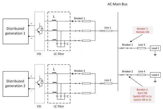
Figure 6.
Second-order system in simulation.
The method described in this paper and previous publications has been verified experimentally using a scale-down system with two distributed generators.
In the experiment, total load demands are Ptotal = 1200 W, Qtotal = 100 Var, VLL(RMS) = 90 V, and Vdc = 180 V.
Figure 7 is the system set-up, which contains one grid-forming and another grid-supporting generator; each one is powered by a separate DC source. AC loads are not visible within the figure and are at another side of the bench.
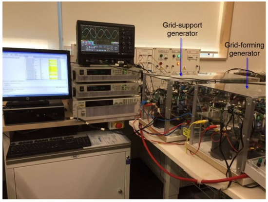
Figure 7.
Experiment setup.
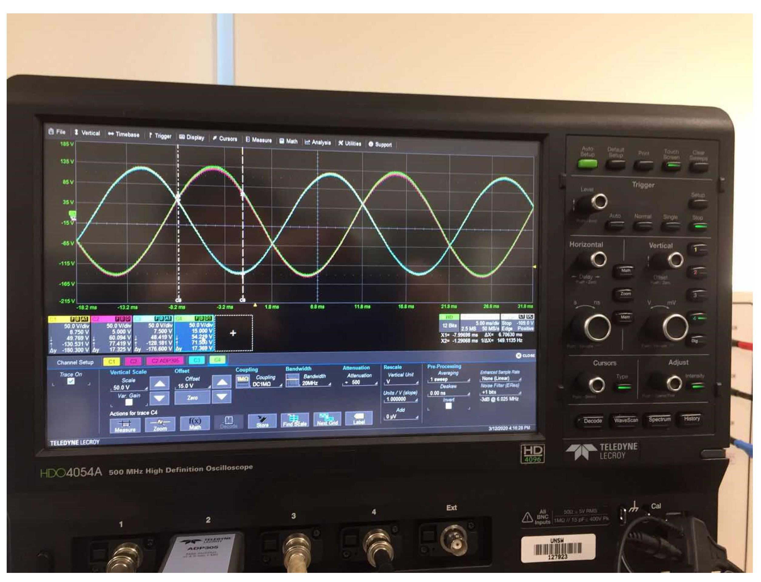
Figure 8 shows the wave-shapes of line-line voltage ab and bc from the AC bus after two generators are connected.
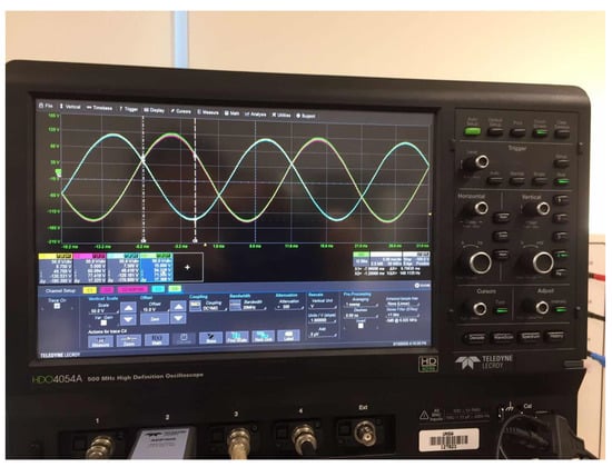
Figure 8.
The ab and bc line-line voltages at the AC bus after synchronization.
The grid-forming generator is started up with an R-L load. Then, the grid-supporting generator is synchronized with the voltages at the AC bus, and breakers are closed to join the grid-supporting generator to the grid-forming one. It is found that, by setting the reactive power reference to a percentage, around 20% of its real power output in the grid-supporting generator, its output can follow such a reference accurately. The remaining reactive power required by the overall loads comes automatically from the grid-forming generator. This reactive power balance between generations and load demand observed in the experiment is the same as that in the simulation.
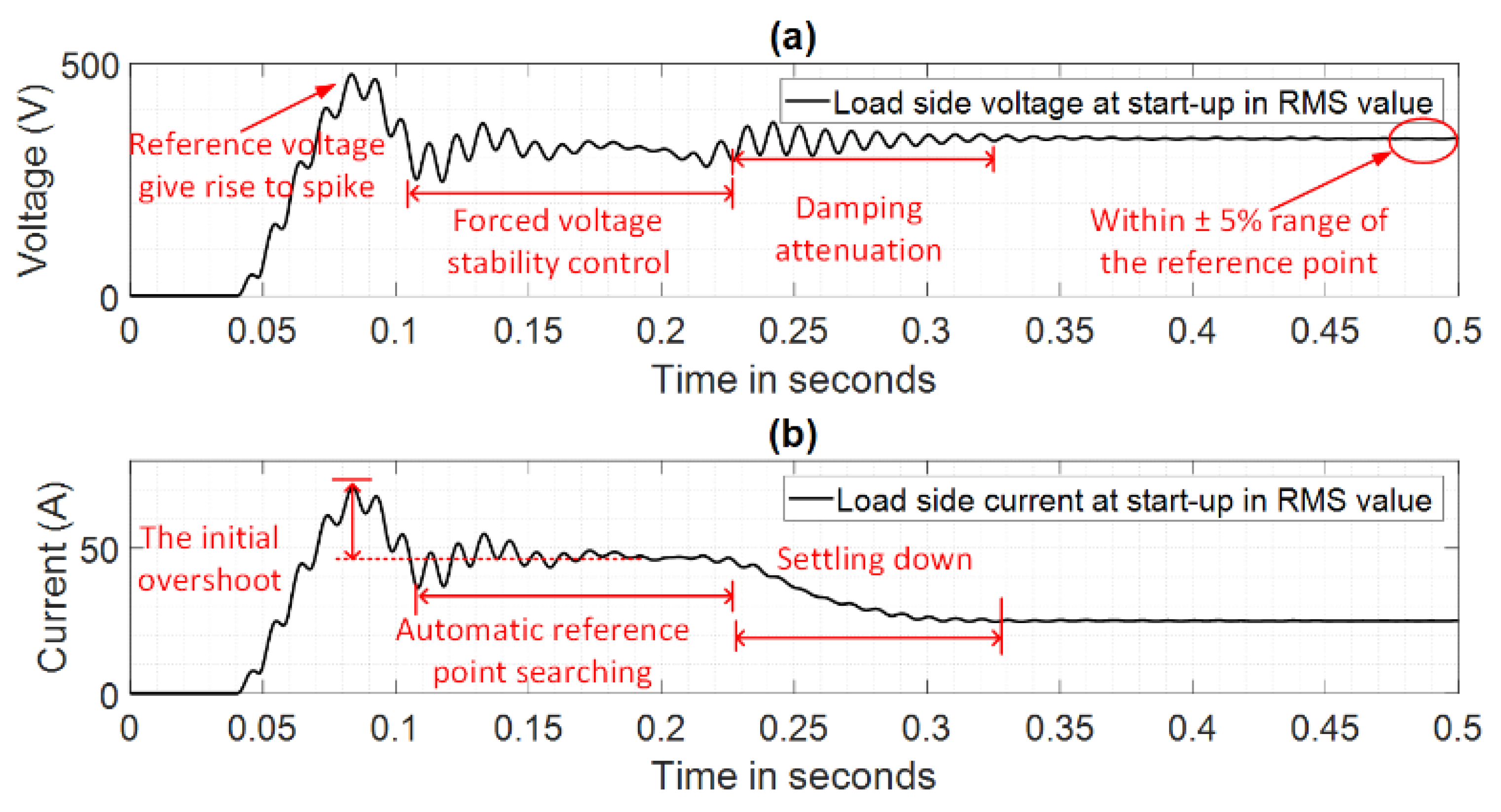
At the start-up shown in Figure 9, the grid-support generator needs to have a proper KV1, as shown in Equation (54) below, to reach the same voltage level at the AC bus produced by the grid-forming generator.
where Vref can be set slightly above the rated voltage of the system.
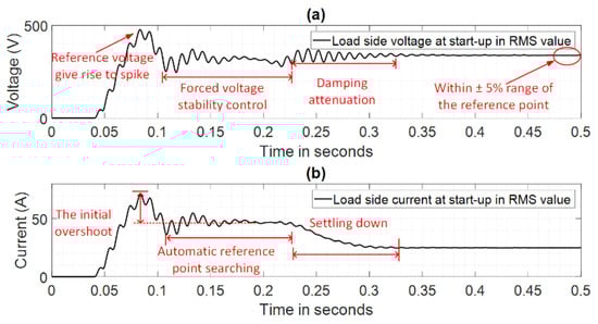
Figure 9.
System starts up. (a) Preliminary voltage from the fixed load, (b) preliminary current from the fixed load.
After being grid-connected, KV1 for the grid-support generator needs to be adjusted step-by-step properly to achieve equal real-power sharing with the grid-forming generator. Such values can be obtained from calibration.
Moreover, another factor KV2, as shown in (55) and (56), can be adopted to cope with the contradiction between transient stability and steady-state error. With such a factor introduced, one may reduce the value of the control parameter Kp1. By doing so, when there is a transient owing to loads’ switch-in or switch-off, and so on, the system can avoid running into instability. Nevertheless, such a reduction of Kp1 leads to higher steady-state voltage error, thereby compromising power quality. After transient, by adjusting KV2, the error can be reduced to within the limit under different loading levels. The effect of introducing KV2 is equivalent to varying Vref to improve the voltage profile under steady state.
The L-C filter is used for both inverters in the experiment. For a safe operation, passive damping is always indispensable by connecting a small resistance in series with a shunt capacitor if the DC source can provide very large current. Without such damping resistance, the catastrophic resonant voltage could occur.
In our system, 5 kHz is used as the switching frequency. It works for the low voltage level up to 90 V (LL). For higher voltage applications, it is necessary to increase the sampling frequency.
Microgrid system parameters are provided in Table 1. Calculated controller parameters are given in Table 2.

Table 1.
Microgrid system parameters.
Table 2.
Microgrid control parameters.
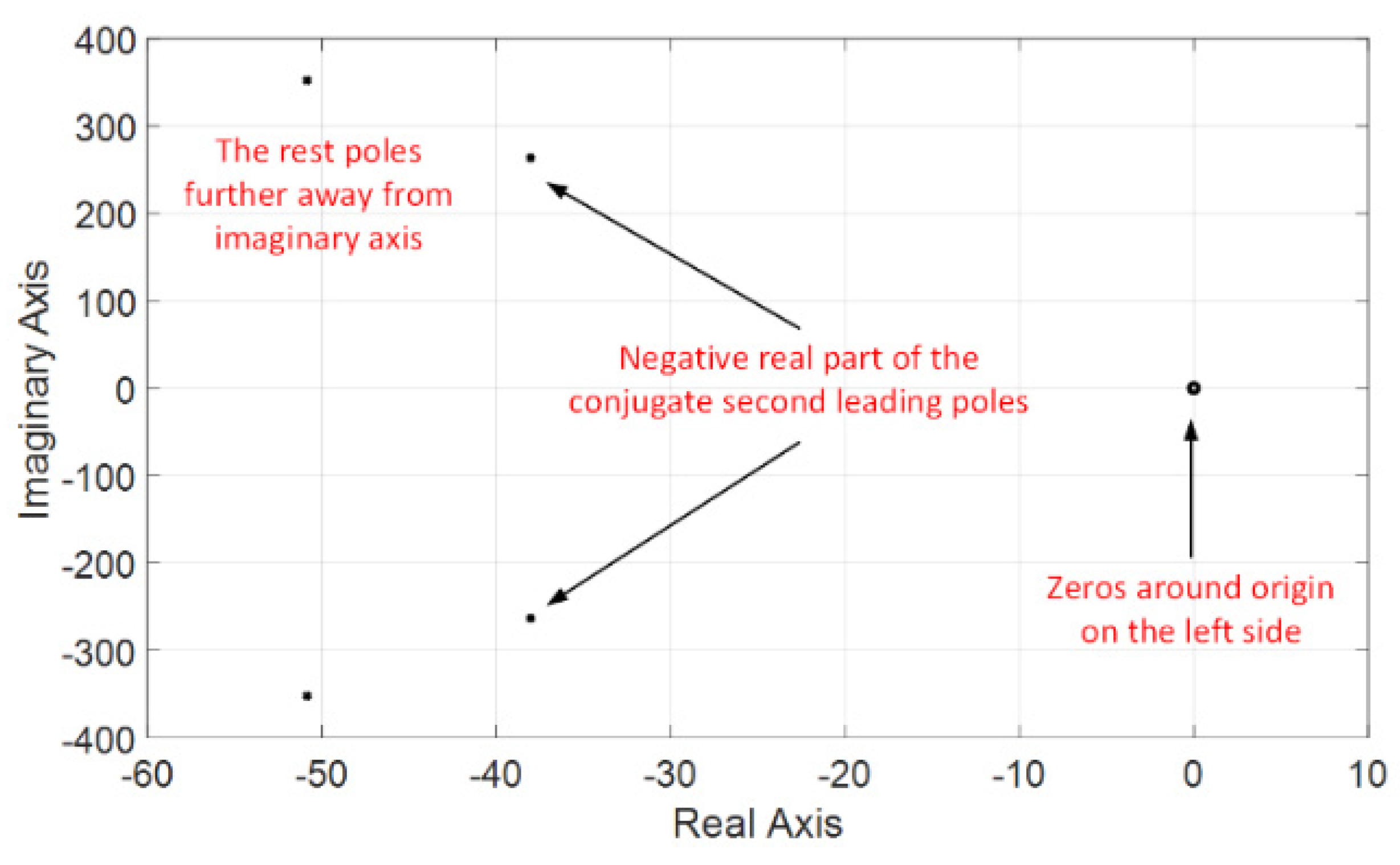
The system stability feature in Figure 10 obviously shows that all the poles lie on the negative half-plane after the first pole, indicating the stable nature of this autonomous system.
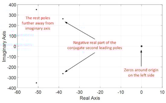
Figure 10.
Pole zero map.
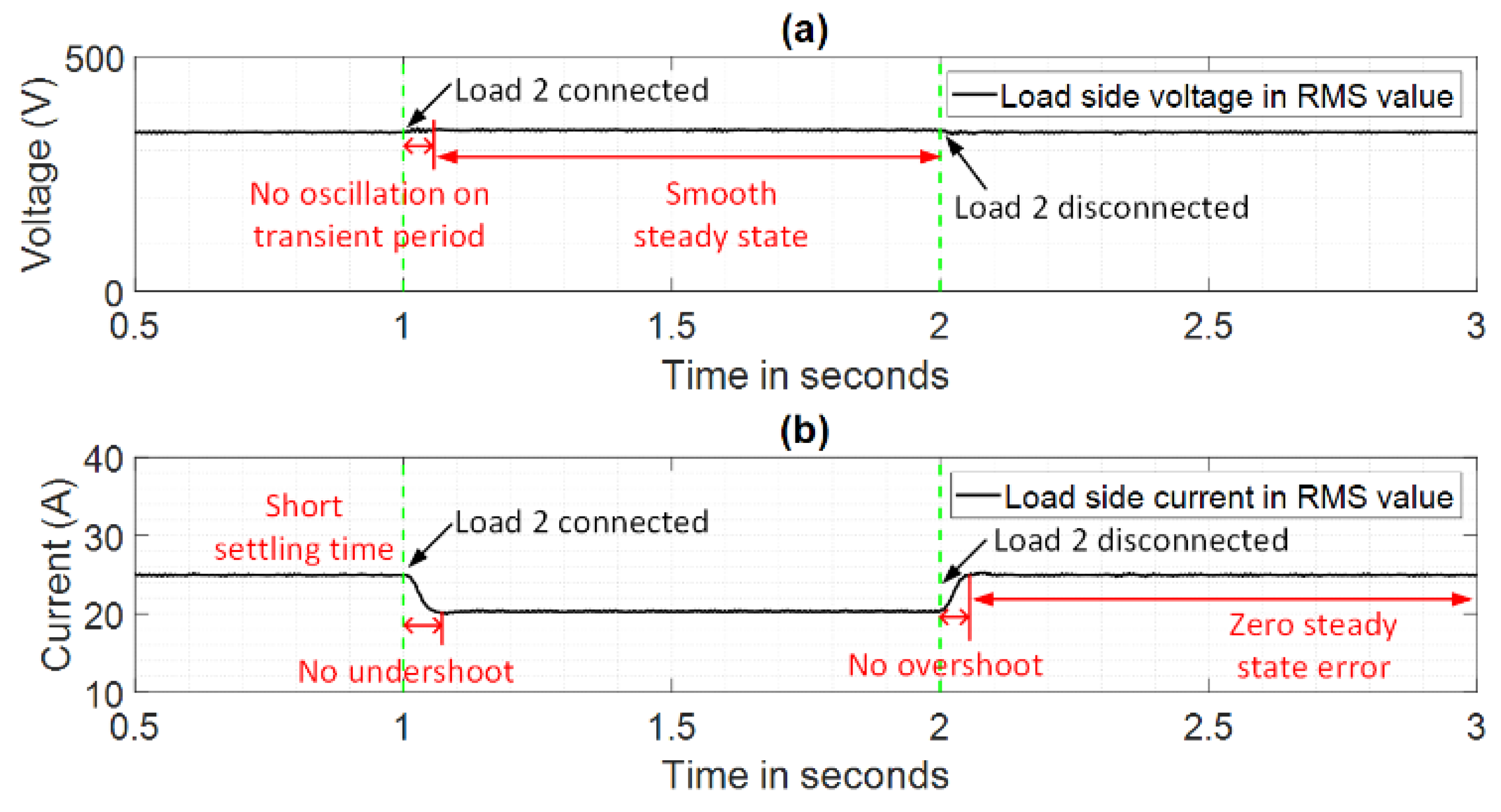
Figure 11 implies the system voltage–current response. Steady-state switchover becomes smoother after the initial start-up. In the voltage control loop, voltage is regulated at 415 V nominal voltage, with slightly deviations for V-P control tuning. In the first second, loads 1 and 2 are both connected, requiring 25 kW active power. At 1 s, load 2 is disconnected, so that the load demand is decreased to only 20 kW. As the voltage is kept at a fixed value, the decoupled current regulation in d-q frame tracks the new current reference calculated by the new active power reference. Thus, the load current decreases from 1 to 2 s. From 2 s, load 2 is reconnected, so that the reference active power and reference current increase at the same time to satisfy the two loads.
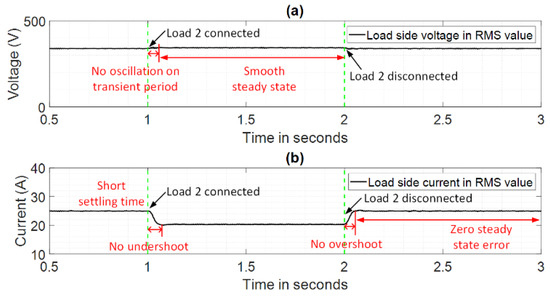
Figure 11.
Load voltage and current. (a) Voltage from the load side, (b) current from the load side.
6.1. System Responses to Switching Loads
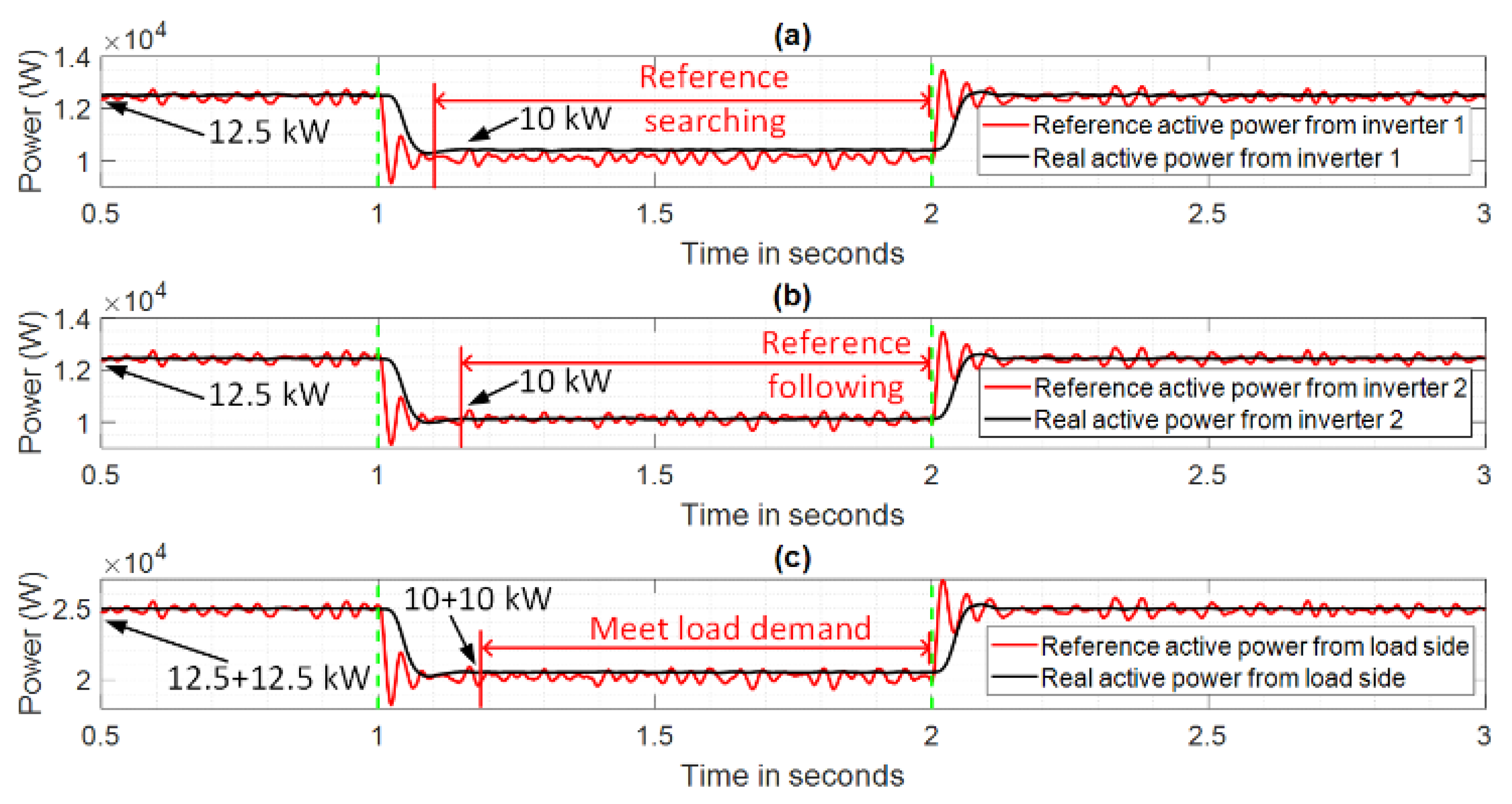
For a fixed coefficient , we switch load 2 off at 1 s and on at 2 s. The results in Figure 12 and Figure 13 show satisfying tracking and response performance. Figure 12 is the multiplication form with a certain adjustment factor from Figure 11, because it is the active power from the generation side. The red line is the reference active power calculated by the V-P control algorithm; the black line is the actual active power from the generation side. Figure 12c is the total active power, which is 25 kW with both loads connected at 0–1 and 2–3 s, and becomes 20 kW with load 1 connected at 1–2 s. Power generator 1 and 2 have equal power sharing between each other, sharing half of the total active power demand. Therefore, (a) and (b) represent generator 1 and generator 2, respectively. Both of them track 12.5 kW well before 1 s and after 2 s, and track 10 kW between 1 and 2 s. This power change is caused by load switches on and off.
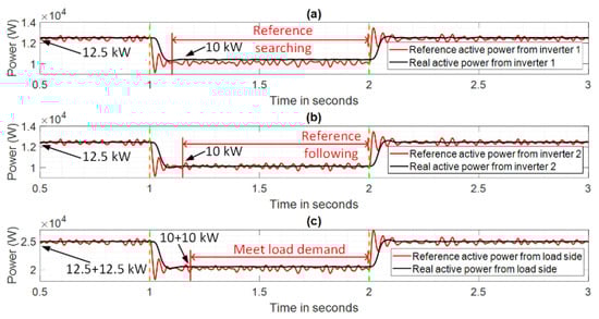
Figure 12.
Active power tracking result with measured active power (black) and reference active power (red). (a) Active power from the first generator, (b) active power from the second generator, (c) total active power.
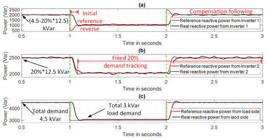
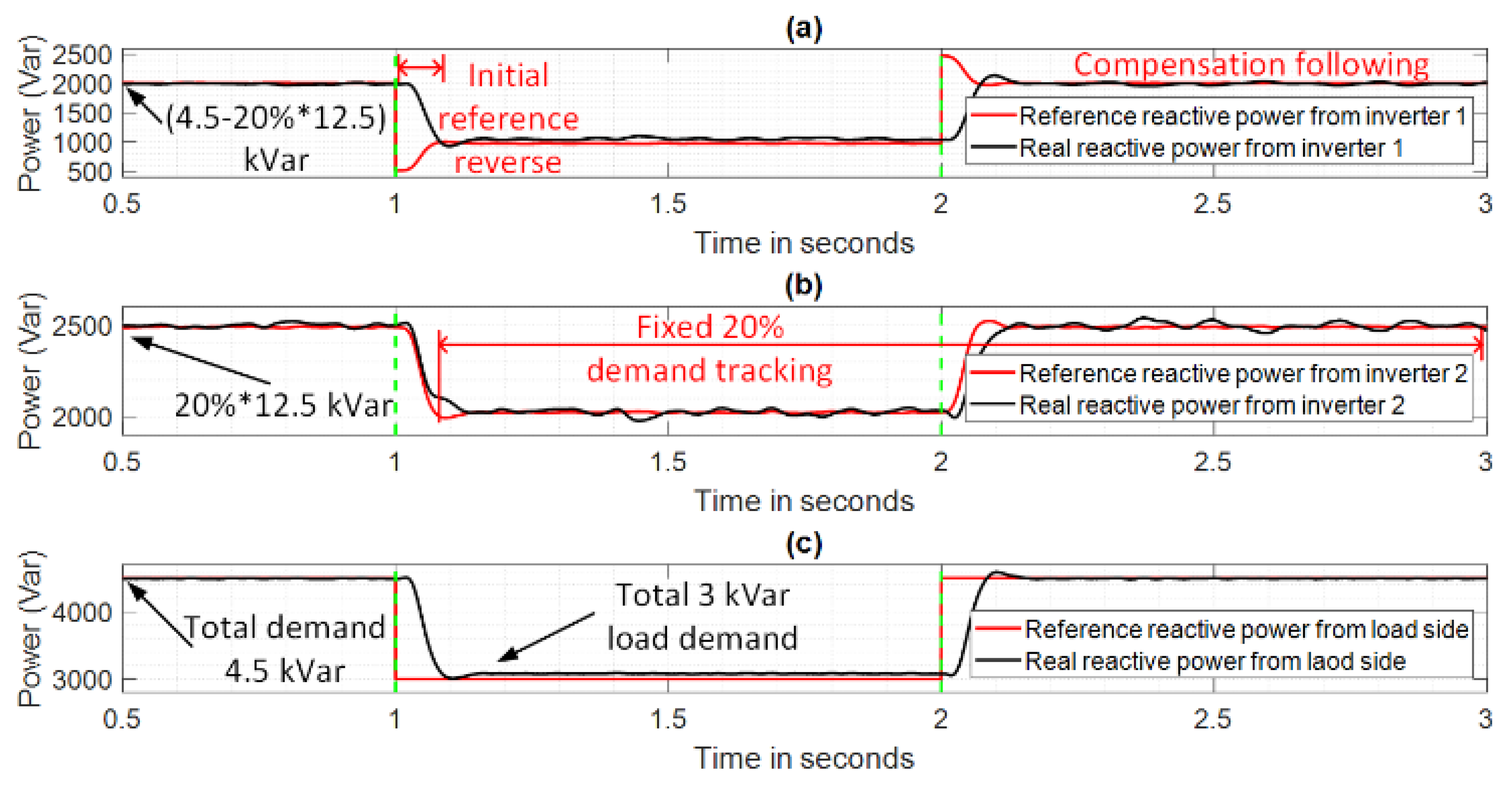
Figure 13.
Reactive power tracking result with measured reactive power (black) and reference reactive power (red). (a) Reactive power from the first generator, (b) reactive power from the second generator, (c) total reactive power.
As shown in Figure 12, three figures track active power in the first inverter, the second inverter, and both inverters in total. The red line shows the reference, while black is a measured value. Three plots indicate suitable tracking, but references have more volatility than real power. This is because the reference calculation does not involve filters, only affecting control inputs instantaneously, but the real measured value is after the LC filter with a smoother appearance. Furthermore, two generations have equal power-sharing for the 2.5 kW power drop when load switches.
In Figure 13, displaying reactive power tracking, reactive power in grid-supporting generators tracks the given percentage of measured active power 12.5 kW, which is 2.5 kW before load switches. After the first second, reactive power is 20% of 10 kW, which is 2 kW. Finally, it turns back to 2.5 kW.
The grid-forming generators compensate for the rest. At the beginning and end, it is 4.5 kW − 2.5 kW = 2 kW. During the first and second seconds, it drops to 3 kW − 2 kW = 1 kW.
The last plot in Figure 13 shows the ideal numerical reactive power reference and its proper tracking. It is clear that two inverters are unbalanced reactive power provider, where the ratio depends on . This is usually selected at around 0–40%. In Figure 13, is chosen to be 20%. That is, if the total reactive power demand is 4.5 kVar at 0–1 s, power generator 2 provides 20% ∗ 12.5 kVar = 2.5 kVar, and power generator 1 tracks the remaining 4.5 – 2.5 = 2 kVar. At 1–2 s, the reactive power demand required by load 2 only is 3 kVar, power generator 2 gives 20% ∗ 10 kVar = 2 kVar, and power generator 1 follows the remaining 1 kVar. In a later section, the influence caused by variation is discussed. The total reactive power tracking is constant, and changes the ratio of reactive power provided by power supply 1 to 2. This particular power tracking result is unique to this V-P control method.
6.2. Influence of Coefficients and
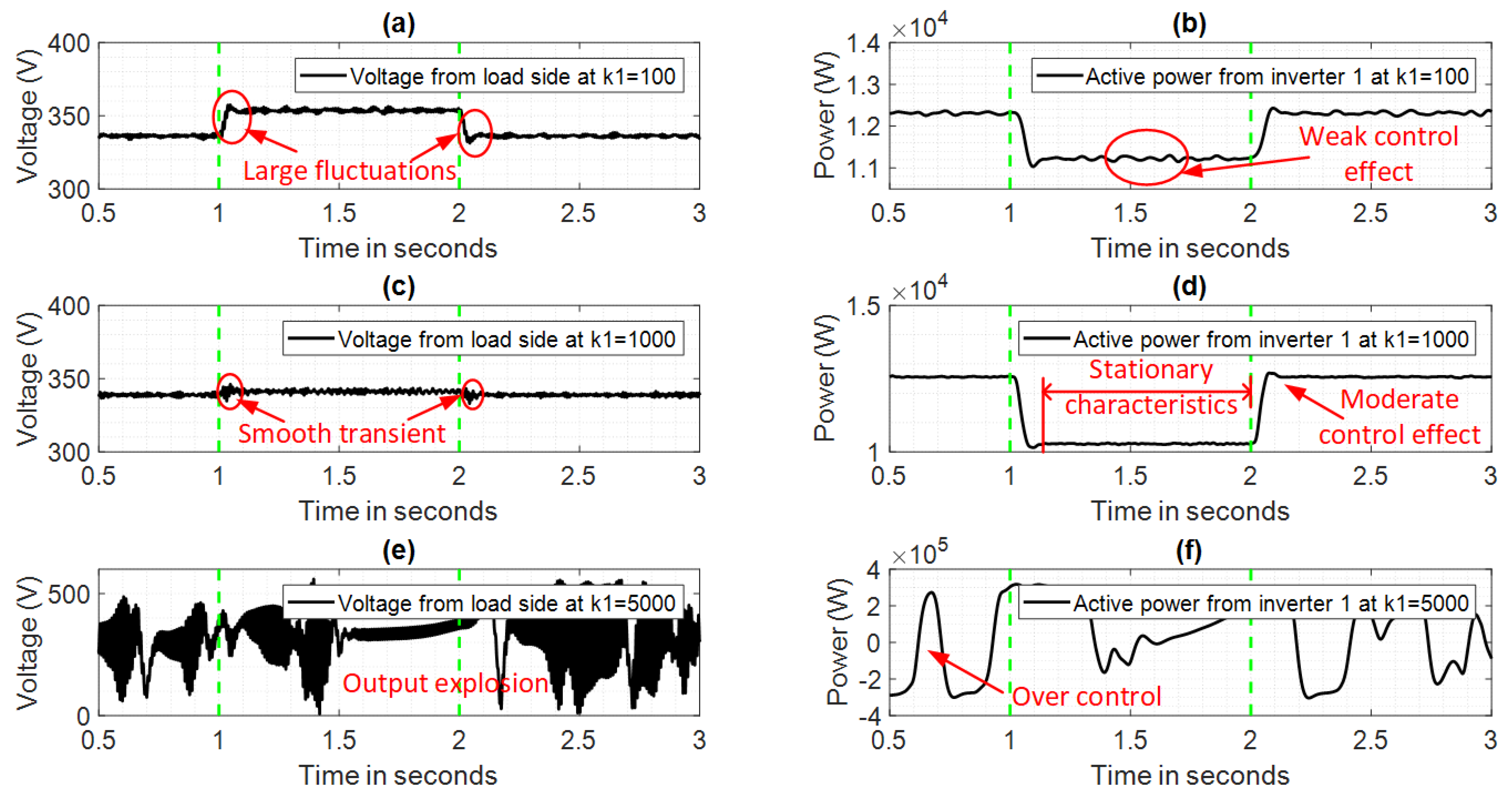
Now, we change coefficient and . The results for increasing are compared in Figure 14. is fixed at 0.2.
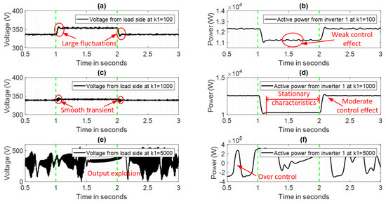
Figure 14.
varying result. (a) Measured voltage in inverter 1 when , (b) measured active power in inverter 1 when , (c) measured voltage in inverter 1 when , (d) measured active power in inverter 1 when , (e) measured voltage in inverter 1 when , (f) measured active power in inverter 1 when .
Figure 14 suggests that, for a more significant coefficient , the system reacts faster and smoother owing to the higher weight on voltage deviation. This leads to more control input and faster power tracking, as seen from the transient period in Figure 14.
However, the system tends to be unstable for a too large coefficient from the last plot in Figure 14. This would have an opposite control effect. Thus, coefficient can be increased as much as possible within its limits for more efficient tracking.
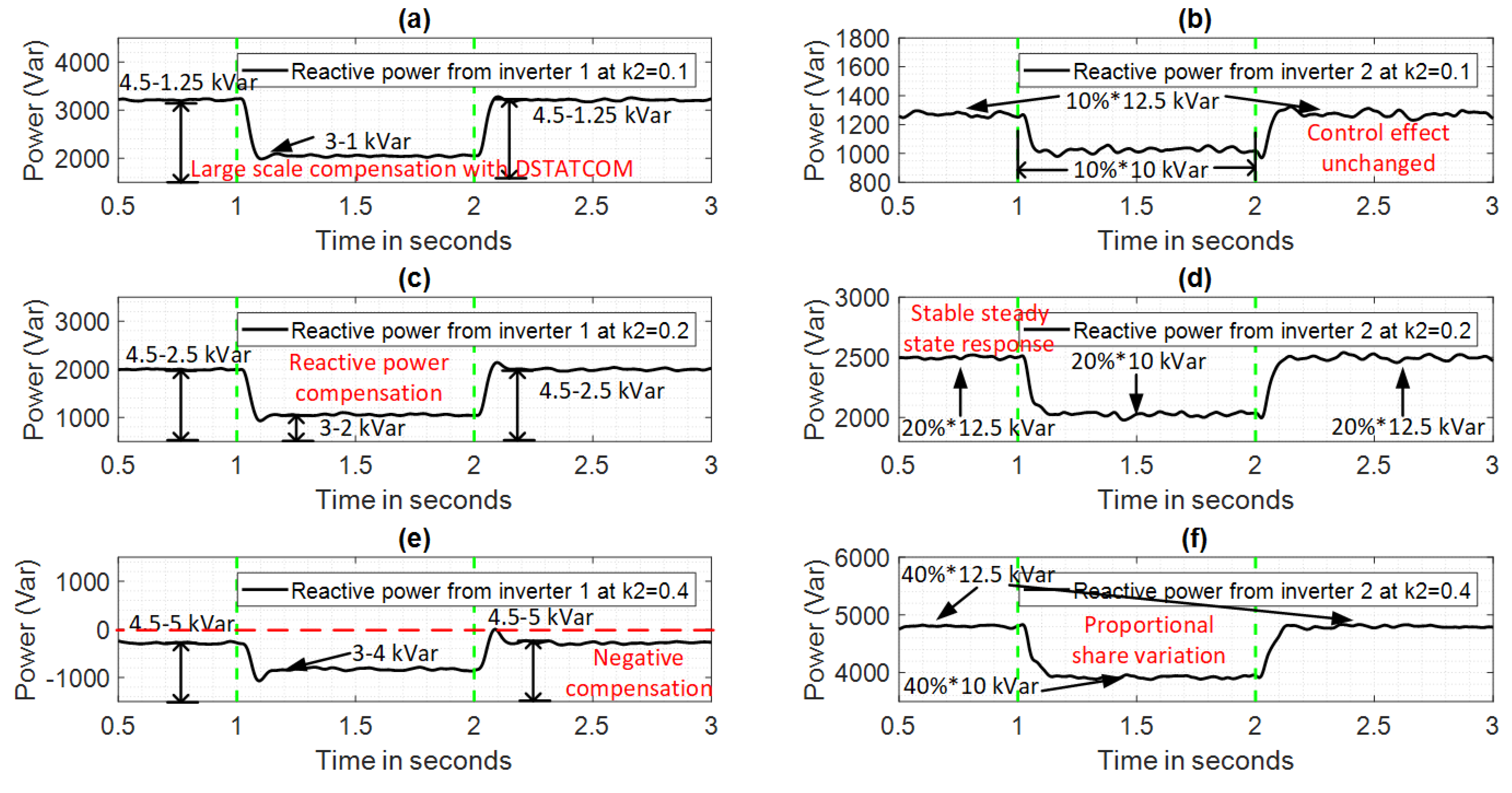
The results for increasing are compared in Figure 15. is fixed at 500. is the proportion of reactive power in measured active power. The total reactive power satisfies load demand, while reactive power in the second source tracks the percentage reference referentially and that in the first source fills the rest. increases by 10%, 20%, and 40%, leading to more dramatic weight on the second source, causing the first source to compensate less. The sum of the active power in two inverters remains unchanged.
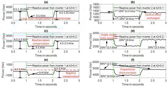
Figure 15.
varying result. (a) Measured reactive power in inverter 1 when , (b) measured reactive power in inverter 2 when , (c) measured reactive power in inverter 1 when , (d) measured reactive power in inverter 2 when , (e) measured reactive power in inverter 1 when , (f) measured reactive power in inverter 2 when .
7. Conclusions
This paper provides a detailed small-signal analysis for the multiple inverters’ multiple loads connected to an islanded AC system using voltage against the active power control method.
Previous research on power control in the AC microgrid usually focused on the droop method or master-slave structure. The double control in voltage and frequency regulation allows for more computation and higher uncertainty. Our adopted method possesses advantages of consuming only a short amount of time, high reliability, superior tracking result, adjustable coefficients, and a flexible system structure.
The main contribution in the paper concerns the derivation of the primary and secondary level small-signal state-space model, various stability analyses, controller test, and coefficient influence study. Simulation and experimental verification were carried out to test practicality and reliability.
It is found that the overall system stability depends on the individual inverter. influence the weight on the degree of participation of voltage in the control, while a larger in bound pushes the system to function faster and more smoothly. Coefficient changes the reactive power percentage in grid supporting generation.
Future work should be directed towards updating the algorithm, controller optimization, and hardware adaptation. This paper provides a theoretical and mathematical foundation for future researchers in this field. In the coming market, the control technique in this paper is prospective in sophisticated microgrids, especially for systems with heavy load switching.
Author Contributions
Conceptualization, X.T. and D.Z.; methodology, X.T.; validation, X.T., D.X. and M.L.; formal analysis, M.L.; resources, D.X.; writing—original draft preparation, X.T. and D.Z.; writing—review and editing, D.Z., D.X. and M.L.; supervision, D.Z.; project administration, D.Z. All authors have read and agreed to the published version of the manuscript.
Funding
This research received no external funding.
Conflicts of Interest
The authors declare no conflict of interest.
References
- Olivares, D.E.; Mehrizi-Sani, A.; Etemadi, A.H.; Cañizares, C.A.; Iravani, R.; Kazerani, M.; Hajimiragha, A.H.; Gomis-Bellmunt, O.; Saeedifard, M.; Palma-Behnke, R.; et al. Trends in microgrid control. IEEE Trans. Smart Grid 2014, 5, 1905–1919. [Google Scholar] [CrossRef]
- Lasseter, R. MicroGrids. In Proceedings of the IEEE Power Engineering Society Winter Meeting Conference, New York, NY, USA, 27–31 January 2002. [Google Scholar]
- Rocabert, J.; Luna, A.; Blaabjerg, F.; Rodriguez, P. Control of power converters in AC microgrids. IEEE Trans. Power Electron. 2012, 27, 4734–4749. [Google Scholar] [CrossRef]
- de Souza, A.C.; Santos, M.; Castilla, M.; Miret, J.; de Vicuña, L.G.; Marujo, D. Voltage Security in AC Microgrids: A Power Flow-Based Approach Considering Droop-Controlled Inverters. In IET Renewable Power Generation; The Institution of Engineering and Technology: Hertford, UK, 2015; Volume 9, pp. 954–960. [Google Scholar]
- Xia, Y.; Peng, Y.; Wei, W. Triple Droop Control Method for Ac Microgrids. In IET Power Electronics; The Institution of Engineering and Technology: Stevenage, UK, 2017; Volume 10, pp. 1705–1713. [Google Scholar]
- Chandorkar, M.C.; Divan, D.M.; Adapa, R. Control of parallel connected inverters in standalone AC supply systems. IEEE Trans. Ind. Appl. 1993, 29, 136–143. [Google Scholar] [CrossRef]
- Tuladhar, A.; Jin, H.; Unger, T.; Mauch, K. Control of parallel inverters in distributed AC power systems with consideration of line impedance effect. IEEE Trans. Ind. Appl. 2000, 36, 131–138. [Google Scholar] [CrossRef]
- Guerrero, J.M.; Vasquez, J.C.; Matas, J.; De Vicuña, L.G.; Castilla, M. Hierarchical control of droop-controlled AC and DC microgrids—A general approach toward standardization. IEEE Trans. Ind. Electron. 2010, 58, 158–172. [Google Scholar] [CrossRef]
- Tan, K.T.; So, P.L.; Chu, Y.C.; Chen, M.Z. Coordinated control and energy management of distributed generation inverters in a microgrid. IEEE Trans. Power Deliv. 2013, 28, 704–713. [Google Scholar] [CrossRef] [Green Version]
- Wu, D.; Tang, F.; Dragicevic, T.; Vasquez, J.C.; Guerrero, J.M. A control architecture to coordinate renewable energy sources and energy storage systems in islanded microgrids. IEEE Trans. Smart Grid 2014, 6, 1156–1166. [Google Scholar] [CrossRef] [Green Version]
- Du, W.; Lasseter, R.H.; Khalsa, A.S. Survivability of autonomous microgrid during overload events. IEEE Trans. Smart Grid 2018, 10, 3515–3524. [Google Scholar] [CrossRef]
- Marwali, M.N.; Jung, J.W.; Keyhani, A. Control of distributed generation systems-Part II: Load sharing control. IEEE Trans. Power Electron. 2004, 19, 1551–1561. [Google Scholar] [CrossRef]
- Wang, Y.; Wang, X.; Chen, Z.; Blaabjerg, F. Distributed optimal control of reactive power and voltage in islanded microgrids. IEEE Trans. Ind. Appl. 2017, 53, 340–349. [Google Scholar] [CrossRef]
- Mahmood, H.; Michaelson, D.; Jiang, J. Accurate reactive power sharing in an islanded microgrid using adaptive virtual impedances. IEEE Trans. Power Electron. 2014, 30, 1605–1617. [Google Scholar] [CrossRef]
- Lu, X.; Wang, J.; Guerrero, J.M.; Zhao, D. Virtual- impedance-based fault current limiters for inverter dominated AC microgrids. IEEE Trans. Smart Grid 2016, 9, 1599–1612. [Google Scholar] [CrossRef] [Green Version]
- Guerrero, J.M.; De Vicuna, L.G.; Matas, J.; Castilla, M.; Miret, J. Output impedance design of parallel-connected UPS inverters with wireless load-sharing control. IEEE Trans. Ind. Electron. 2005, 52, 1126–1135. [Google Scholar] [CrossRef]
- Yao, W.; Chen, M.; Matas, J.; Guerrero, J.M.; Qian, Z.M. Design and analysis of the droop control method for parallel inverters considering the impact of the complex impedance on the power sharing. IEEE Trans. Ind. Electron. 2010, 58, 576–588. [Google Scholar] [CrossRef]
- Tao, Y.; Liu, Q.; Deng, Y.; Liu, X.; He, X. Analysis and mitigation of inverter output impedance impacts for distributed energy resource interface. IEEE Trans. Power Electron. 2014, 30, 3563–3576. [Google Scholar] [CrossRef]
- Zhang, D. Operation of microgrid at constant frequency with a standby backup grid-forming generator. In Proceedings of the 2016 IEEE International Conference on Power System Technology (POWERCON), Wollongong, Australia, 28 September–1 October 2016; pp. 1–6. [Google Scholar]
- Zhang, D.; Fletcher, J. Operation of autonomous AC microgrid at constant frequency and with reactive power generation from grid-forming, grid-supporting and grid-feeding generators. In Proceedings of the TENCON 2018–2018 IEEE Region 10 Conference, Jeju, Korea, 28–31 October 2018; pp. 1560–1565. [Google Scholar]
- Tang, X.; Zhang, D. Islanded AC Microgrid Stability and Feasibility Analysis on VP Control with Estimation at Constant Frequency. In Proceedings of the 2019 9th International Conference on Power and Energy Systems (ICPES), Perth, Australia, 10–12 December 2019; pp. 1–6. [Google Scholar]
- Lee, C.T.; Chu, C.C.; Cheng, P.T. A new droop control method for the autonomous operation of distributed energy resource interface converters. IEEE Trans. Power Electron. 2012, 28, 1980–1993. [Google Scholar] [CrossRef]
- Lee, C.T.; Chu, C.C.; Cheng, P.T. Quantitative analysis of system parameters asymmetry on droop-controlled converters. In Proceedings of the 2012 IEEE Energy Conversion Congress and Exposition (ECCE), Raleigh, NC, USA, 15–20 September 2012; pp. 2381–2388. [Google Scholar]
- Zhou, J.; Cheng, P.T. A Modified Q—Droop Control for Accurate Reactive Power Sharing in Distributed Generation Microgrid. IEEE Trans. Ind. Appl. 2019, 55, 4100–4109. [Google Scholar] [CrossRef]
- Paquette, A.D.; Divan, D.M. Virtual impedance current limiting for inverters in microgrids with synchronous generators. IEEE Trans. Ind. Appl. 2014, 51, 1630–1638. [Google Scholar] [CrossRef]
- Paquette, A.D.; Reno, M.J.; Harley, R.G.; Divan, D.M. Sharing transient loads: Causes of unequal transient load sharing in islanded microgrid operation. IEEE Ind. Appl. Mag. 2013, 20, 23–34. [Google Scholar] [CrossRef]
- Majumder, R.; Chaudhuri, B.; Ghosh, A.; Majumder, R.; Ledwich, G.; Zare, F. Improvement of stability and load sharing in an autonomous microgrid using supplementary droop control loop. IEEE Trans. Power Syst. 2009, 25, 796–808. [Google Scholar] [CrossRef] [Green Version]
- Yazdanian, M.; Mehrizi-Sani, A. Washout filter-based power sharing. IEEE Trans. Smart Grid 2015, 7, 967–968. [Google Scholar] [CrossRef]
- Sun, C.; Joos, G.; Bouffard, F. Control of microgrids with distributed energy storage operating in Islanded mode. In Proceedings of the 2017 IEEE Electrical Power and Energy Conference (EPEC), Saskatoon, SK, Canada, 22–25 October 2017; pp. 1–7. [Google Scholar]
- Kolluri, R.R.; Mareels, I.; Alpcan, T.; Brazil, M.; de Hoog, J.; Thomas, D.A. Power sharing in angle droop controlled microgrids. IEEE Trans. Power Syst. 2017, 32, 4743–4751. [Google Scholar] [CrossRef]
- Mondal, A.; Illindala, M.S. Improved frequency regulation in an islanded mixed source microgrid through coordinated operation of DERs and smart loads. IEEE Trans. Ind. Appl. 2017, 54, 112–120. [Google Scholar] [CrossRef]
- Microgrids: Architectures and Control; Wiley: Chichester, UK, 2014.
- Kim, Y.S.; Kim, E.S.; Moon, S.I. Frequency and voltage control strategy of standalone microgrids with high penetration of intermittent renewable generation systems. IEEE Trans. Power Syst. 2015, 31, 718–728. [Google Scholar] [CrossRef]
- Kim, J.Y.; Jeon, J.H.; Kim, S.K.; Cho, C.; Park, J.H.; Kim, H.M.; Nam, K.Y. Cooperative control strategy of energy storage system and microsources for stabilizing the microgrid during islanded operation. IEEE Trans. Power Electron. 2010, 25, 3037–3048. [Google Scholar]
- Manson, S.; Nayak, B.; Allen, W. Robust microgrid control system for seamless transition between grid-tied and island operating modes. In Proceedings of the 44th Annual Western Protective Relay Conference, Spokane, WA, USA, 17–19 October 2017. [Google Scholar]
- Vasquez, J.C.; Guerrero, J.M.; Luna, A.; Rodríguez, P.; Teodorescu, R. Adaptive droop control applied to voltage-source inverters operating in grid-connected and islanded modes. IEEE Trans. Ind. Electron. 2009, 56, 4088–4096. [Google Scholar] [CrossRef]
- He, J.; Li, Y.W.; Blaabjerg, F. An enhanced islanding microgrid reactive power, imbalance power, and harmonic power sharing scheme. IEEE Trans. Power Electron. 2014, 30, 3389–3401. [Google Scholar] [CrossRef]
- He, J.; Li, Y.W.; Guerrero, J.M.; Blaabjerg, F.; Vasquez, J.C. An islanding microgrid power sharing approach using enhanced virtual impedance control scheme. IEEE Trans. Power Electron. 2013, 28, 5272–5282. [Google Scholar] [CrossRef]
- Zhang, H.; Kim, S.; Sun, Q.; Zhou, J. Distributed adaptive virtual impedance control for accurate reactive power sharing based on consensus control in microgrids. IEEE Trans. Smart Grid 2016, 8, 1749–1761. [Google Scholar] [CrossRef]
- Lu, L.Y.; Chu, C.C. Consensus-based droop control synthesis for multiple DICs in isolated micro-grids. IEEE Trans. Power Syst. 2014, 30, 2243–2256. [Google Scholar] [CrossRef]
- Olfati-Saber, R.; Fax, J.A.; Murray, R.M. Consensus and cooperation in networked multi-agent systems. Proc. IEEE 2007, 95, 215–233. [Google Scholar] [CrossRef] [Green Version]
- Zhou, J.; Kim, S.; Zhang, H.; Sun, Q.; Han, R. Consensus-based distributed control for accurate reactive, harmonic, and imbalance power sharing in microgrids. IEEE Trans. Smart Grid 2016, 9, 2453–2467. [Google Scholar] [CrossRef] [Green Version]
- Schiffer, J.; Seel, T.; Raisch, J.; Sezi, T. Voltage stability and reactive power sharing in inverter-based microgrids with consensus-based distributed voltage control. IEEE Trans. Control Syst. Technol. 2015, 24, 96–109. [Google Scholar] [CrossRef] [Green Version]
- Han, R.; Meng, L.; Ferrari-Trecate, G.; Coelho, E.A.; Vasquez, J.C.; Guerrero, J.M. Containment and consensus-based distributed coordination control to achieve bounded voltage and precise reactive power sharing in islanded AC microgrids. IEEE Trans. Ind. Appl. 2017, 53, 5187–5199. [Google Scholar] [CrossRef] [Green Version]
- Zhao, C.; He, J.; Cheng, P.; Chen, J. Consensus-based energy management in smart grid with transmission losses and directed communication. IEEE Trans. Smart Grid 2016, 8, 2049–2061. [Google Scholar] [CrossRef]
- Dreidy, M.; Mokhlis, H.; Mekhilef, S. Inertia response and frequency control techniques for renewable energy sources: A review. Renew. Sustain. Energy Rev. 2017, 69, 144–155. [Google Scholar] [CrossRef]
- Bevrani, H.; Ise, T.; Miura, Y. Virtual synchronous generators: A survey and new perspectives. Int. J. Electr. Power Energy Syst. 2014, 54, 244–254. [Google Scholar] [CrossRef]
- Zhang, D. Issues on load shedding in a microgrid operated at constant frequency. In Proceedings of the 2017 20th International Conference on Electrical Machines and Systems (ICEMS), Sydney, Australia, 11–14 August 2017; pp. 1–5. [Google Scholar]
- Coelho, E.A.A.; Cortizo, P.C.; Garcia, P.F.D. Small-signal stability for parallel-connected inverters in stand-alone AC supply systems. IEEE Trans. Ind. Appl. 2002, 38, 533–542. [Google Scholar] [CrossRef]
- Coelho, E.A.A.; Cortizo, P.C.; Garcia, P.F.D. Small signal stability for single phase inverter connected to stiff AC system. In Proceedings of the Conference Record of the 1999 IEEE Industry Applications Conference. Thirty-Forth IAS Annual Meeting (Cat. No. 99CH36370), Phoenix, AZ, USA, 3–7 October 1999; Volume 4, pp. 2180–2187. [Google Scholar] [CrossRef]
- Tang, X.; Zhang, D.; Chai, H. Synthetical Optimal Design for Passive-Damped LCL Filters in Islanded AC Microgrid. J. Energy Power Technol. 2021, 3, 22. [Google Scholar] [CrossRef]

Publisher’s Note: MDPI stays neutral with regard to jurisdictional claims in published maps and institutional affiliations. |
© 2021 by the authors. Licensee MDPI, Basel, Switzerland. This article is an open access article distributed under the terms and conditions of the Creative Commons Attribution (CC BY) license (https://creativecommons.org/licenses/by/4.0/).