Abstract
In this article, methods of formation maintenance for a group of autonomous agents under ageneral topology scheme are discussed. Unlike rendezvous or geometric formation, general topology pursuit allows the group of agents to autonomously form trochoid patterns, which are useful in civilian and military applications. However, this type of topology is established by designing a marginally stable system that may be sensitive to parameter variations. To account for this drawback of stability, linear fixed-gains are turned into a dynamical version in this paper. By implementing a disturbance observer controller, systems are shown to maintain their formation despite the disturbances or uncertainties. Comparison in the effectiveness of the presented method with model reference adaptive control and integral sliding mode control under the uncertainties of the gains is also conducted. The capabilities of controllers are demonstrated and supported through simulations.
1. Introduction
A multi-agent system (MAS) is made up of a fleet of agents that collaborate under a set of designed rules. In fields such as space-based applications, smart grids, and machine learning, multi-agent systems employ networked numerous autonomous agents to complete complicated tasks, where local interactions among the agents are used to achieve an overall goal. Agents can be ships [1], unmanned vehicles [2], cars [3], or also satellites, for whom numerous projects for Earth observations needing MAS were conducted in recent years [4,5].
Out of the various tasks that are required for MAS, formation control witnessed ample development. The formation control is defined as coordinated supervision for a group of agents to follow a predefined trajectory while maintaining a desired spatial pattern or accomplishing designed objectives such as target circling, formation-shape maintenance, reorganizing shape, agent-fault detection, or consensus [6,7,8]. Consensus, or agreement concordat, have been actively studied using the so-called cyclic pursuit (CP) protocol. Cyclic pursuit is a simple leaderless distributed control law, consisting of a group of n agents, where each agent uses its neighboring agents’ information to compute its velocity or acceleration vector. These autonomous groups use local interactions to render global formations.
Amid the studies of cyclic pursuit, circular pattern generation and preservation is an up-to-date topic among researchers. In [9], by measuring a desirable relative phase angle between neighbors, the suggested controller directs a team to circumnavigate an arbitrary distribution of target points at a specified radius from the targets. Authors in [10] present a control method based on the chasing agent’s bearing angle knowledge and preserve the inter-agent distance between the agents in a heterogeneous manner. The study conducted in [11] examines the circular formation control issue of MAS in order to achieve any predetermined phase distribution. The proposed control law drives all of the agents to a circle and arranges them in places dispersed on the circle based on preset relative phases. In [12], the challenge of surrounding and monitoring a moving object using a fleet of unicycle-like vehicles is addressed. By using agents’ communication, the developed controller guides the vehicles into an equally spaced formation along a circle, the center of which follows the target’s motion. Scientists in [13] used a team of under-actuated vehicles to guarantee that a moving target is circled uniformly with the required radius, velocity, and inter-vehicle spacing. In these geometric formations, the agents attain and maintain a preset relative distance. By nature, the closed-loop system that generates geometric formation is intrinsically stable.
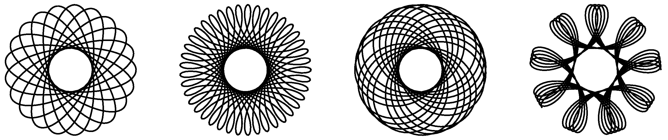
Outside the limits of circular patterns and geometric formation lies the class of trochoid motif. A trochoid can be defined as the curve drawn out by a point fixed to a circle as it rolls down a straight line (the point might be on, inside, or outside the circle, see Figure 1). In addition to their aesthetic appeals, these trajectories are helpful in a variety of civil and military purposes, as every point on an annular area in a plane can be covered by the trajectories. As a result, a group of agents may conduct activities such as search, exploration, surveillance, patrolling, monitoring, and other similar civilian usages, as well as cleaning and grass mowing [14,15,16].
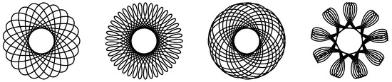
Figure 1.
Trochoidal-like curves.
Multi-agents systems using a protocol to generate these trochoid behaviors are marginally stable per se. Pavone and Frazzoli showed that n agents eventually converge to a single point, a circle, or diverge following a logarithmic spiral pattern under specific conditions for the value of the gain (the word gain refers to tuning parameter) [17]. It leads the overall network to have purely imaginary axis eigenvalues. The requirement of possessing imaginary-axis eigenvalues is also the backbone of Tsiotras’ paper where it was shown that a marginally stable system is a magnificent and simple way to generate artistic patterns [18]. Juang carried out the analysis and added a new rigidity gain, leading also to a multiple imaginary-axis eigenvalues configuration, which renders a class of epicycle patterns. This configuration was used in a dynamic coverage scheme, where agents stay within a certain area and ensure a minimum time between two passages over the same point [19,20]. Moses et al. kept the investigation of geometric pattern formation by manipulating the location of the eigenvalues of the overall system while keeping multiple-axis eigenvalues. Further, the law to achieve trochoidal pattern formation was generalized to render such patterns under a generalized topology pursuit (GTP), and the pattern formation was extended to three dimensions space [21,22]. The reason for this expansion was illustrated by demonstrating that, given general graph topologies, the agents may span areas of varying circular radii.
The crucial point is to ensure the gains’ stability as they are the gatekeeper of the network formation. The criteria of having purely imaginary eigenvalues, and all the remaining in the left half complex plane are decisive in trochoid patterns generation. Such a marginally stable configuration relies only on the gains value’s selection. The aforementioned gains are fixed and can be subject to uncertainties, which is a limitation. Thus, the challenge of maintaining the marginal stability of such networks under some bounded disturbances on the gains arose.
Control techniques such as adaptive control or dynamic gains approach were developed for MAS. In [23], authors employed time-varying feedback coupling gains in order to synchronize the development of a complex network. In addition, the work conducted in [24] deals with the synchronization of MAS by using weightage based on local information. In [25], the study presents a modified follower’s control rule in which each agent follows its neighbor along a line of sight rotated by a fixed offset angle and with a dynamic control gain. Examples of dynamical control by the application of adaptive approaches for cyclic chase were antecedently covered. The researchers in [26,27] use model reference adaptive control on a MAS under generalized cyclic pursuit (GCP) scheme to keep the formation notwithstanding the current uncertainty. Further, the development of an Integral sliding mode controller (ISC) for GCP was approached with the aim of sustaining the motion [28]. In situ situations were also covered in [29], where authors compared a PID controller with an ISC to maintain the formation of a MAS subjected to constant and time-varying disturbances or commands. The conclusion was made that the ISC presents better stability in case of communication failure.
In this paper, we develop an approach based on a disturbance-based observer control (DOB) to ensure uncertainties’ rejection and formation maintenance; as DOB is one of the most extensively utilized robust motion control methods among many controllers. It can be employed to estimate the torque disturbance of a DC servo speed control system, and its performance has been thoroughly investigated [30,31,32,33,34]. Using a nonlinear controller, authors in [35] used a DOB as well to perform the trajectory tracking of a quadrotor in the presence of external disturbances. Previous methods to ensure the stability of the gains were developed in [26,28] where ISC and MRAC were tested. The latter methods can also be applied to the presented GTP and thus will be tested. In the present study, we enhance the work conducted in [26,28] and show that these methods can be employed in a more general case of communication graph. Through simulations, we compare the performances of DOB, ISC, and MRAC and draw conclusions about the best trade-off.
Notation 1.
The bold mathematical letters define matrix and/or vector. The subscript and are added to help the reader with the size of the squared matrices. The subscript indicates the final value of the variable of interest. The superscript T means transpose. The bold letter i stands for the imaginary number such that ; it should not be mistaken with i, which represents the agents’ identification number. The words pattern/formation are interchangeable as they are used in the same sense.
2. Problem Description
With the aim of helping the reader, a brief overview of graph theory is provided. For a network of n agents communicating with each other, a weighted directed graph can be outlined mathematically by a node set that represents the agents, an edge set that indicates the interaction between the agents, and a weighted adjacency matrix that can be used to store the weights of the edges. In a directed graph, edges link two vertices asymmetrically, while, in an undirected graph, edges link two vertices symmetrically. If agent j can obtain information from agent i, then it is said that an edge exists. The weighted adjacency matrix is defined such that is positive if and 0 otherwise. The set of the interacting neighbor of agents i is denoted by . A directed path of graph is a series of edges that connects a series of vertices. In a directed graph, a directed spanning tree exists if at least one node has a directed path to all other nodes. There are several definitions of the Laplacian matrix in the literature. It is defined as the following real matrix:
where, for all i,
is the diagonal degree matrix, in which
is the weighted in-degree of the vertex v. The Laplacian is symmetric for undirected graphs, while it is not for directed graphs [36].
In order to generate three dimensional trochoidal patterns, consider a group of n leaderless agents whose interactions are based on a weighted directed graph that includes a directed spanning tree. Agents are modeled according to the single integrator kinematics
where denotes the position of i-th agent in Cartesian coordinates, and is the following control law [22]
where is a constant gain,
is the proper rotation matrix by angle around the axis ; a unit vector with , and where and . Equation (5) can be written as the following network
in which is the stacked position vector, and is the state matrix
As the behavior of the system relies on the location of the eigenvalues, the conditions on the gains to place the eigenvalues at desired locations were developed.
As has to be an asymmetric matrix associated with a weighted directed graph having a directed spanning tree, it possesses one zero eigenvalue, and the rest are non-zero eigenvalues with positive real parts [37]. Thereby, taking the negative of the Laplacian will give one zero eigenvalue, and the rest are non-zero eigenvalues with negative real parts. Name the eigenvalues of by , , with and as the corresponding angle of the i-th eigenvalue, arranged such that
In order to obtain the desired eigenvalues position, we name the eigenvalues and such that [22]
In other words, (9a) means that there are no additional eigenvalues on the line connecting and . Similarly, () implies that the line connecting and has no eigenvalues. The three-dimensional rotation matrix in (6) has the following three eigenvalues:
From the properties of the Kronecker product, the eigenvalues of are
where ; see Appendix A for details on the Kronecker product. Finally, the eigenvalues of in (8) are
for . Then, according to ([22], Lemma 4.1, 4.2), to reach the location of specific eigenvalues and thus the desired motion, the following critical values for and must be computed as
and the two pairs of purely imaginary eigenvalues will be distinct if
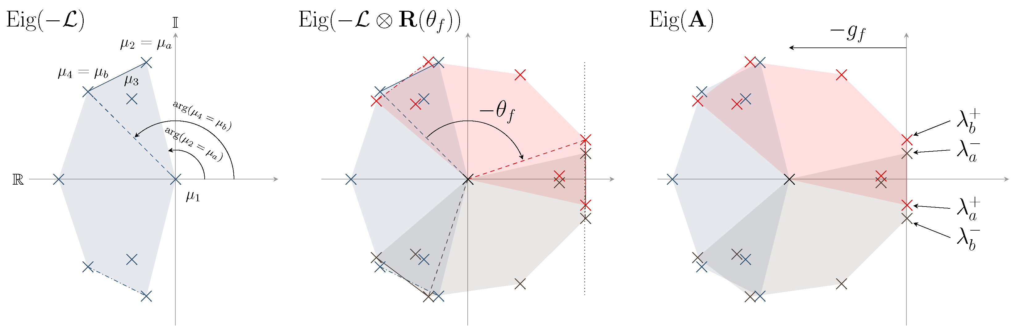
Denoted by are the two pairs of imaginary-axis eigenvalues. A representation of the eigenvalues repartition is drawn on Figure 2, with the right side presenting the eigenvalues of interest .
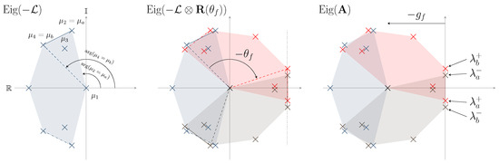
Figure 2.
Evolution of the eigenvalues’ repartition while building the network.
Equation (12) reveals that the eigenvalues repartition depends solely on , which is the key value of the network formation and will be referred to as angle or gain, as its role can be assimilated to a gain value. In its fixed versions presented in [19,22], any perturbations of any agents’ gain would lead to an unstable formation with no way to correct their value. The overall system (7) under uncertain gains is represented by
implying that the problem can be turned into a dynamic version of to reject . In the footsteps of [26,28], we develop a disturbance observer controller to deal with uncertainties and we extend the previously MRAC method to this general network topology. The benefits are the insurance of formation maintenance despite the perturbation possibly encountered in an agent’s gain.
3. Proposed Methods
In the following, different methods are proposed, and we start by the development of the proposed disturbance observer controller, then a review on the integral sliding controller for this specific network [28], and finally by the MRAC method reformulated to match the problem specification. The two former are robust type, while the latter is adaptive type. In DOB-based robust control, Internal and external disturbances are calculated utilizing recognized dynamics and observable gains of agents, and system robustness is easily accomplished by feed-backing disturbance estimations [34]. The sliding mode control is a two-part controller design. The first half is the design and operation of a sliding surface to meet the design requirements, and the second part relates to choosing a control rule that makes the switching surface attractive. By adding an integral term, the system trajectory always starts from the sliding surface, meaning that the reaching phase is eliminated, and robustness over the whole state space is assured [38]. Model reference adaptive control (MRAC) is a direct adaptive strategy with some adjustable controller parameters and an adjusting mechanism to adjust them [39]. These controllers are structurally different and their functioning will be reminded. A first glance of the results is shown on Table 1.

Table 1.
Qualitative comparison between the controllers.
To address the issue of being unable to directly detect disturbances in order to correct them in an open loop, disturbance observers that evaluate disturbances based on observable state variables in the plant and a model of its dynamics were created. The feedback controller was implicitly synthesized to achieve controller robustness by utilizing disturbance estimations rather than their real values. It is feasible to alleviate the measurement of disturbances by using all available past knowledge about the plant model and current measurements of its inputs and outputs. An algorithm for assessing the status of the plant and disturbances was added to the control system for this purpose. The DOB provides a feed-forward compensation term to directly weaken the disturbances in the control systems, by choosing that structure for the observer, one have control over how accurate the estimate is. In the present system, the DOB was applied directly to act on the gains of every agents and can be stated under the following theorem:
Theorem 1.
If a group of n agents modeled by a single integrator are under the control law (5) in which the gains of each agent are set to
with and the eigenvalues following the property (9), a bounded time-varying disturbance, and the controller defined as
where and are positive constant gains appropriately chosen for the heading angle to reach in desired time and the estimated disturbance from the observer. Then at steady-state the eigenvalues of (8) will possess two pairs of imaginary axis eigenvalues and the network (7) will keep its marginal stability despite uncertainties in agents’ gains.
Proof of Theorem 1.
Writing (16a) in terms of state-space form yields
with
and the bounded disturbance, function of and t. The disturbances include perturbation caused by parameter changes, unmodeled dynamics, external disturbances, and consider that they satisfy the matching criterion. In addition, assume that, as t increases, the derivatives of the disturbances tend to certain constants.
The controller will be separated into two components such that
where is the nominal controller and the disturbances estimate peculiar to agent i.
Consider first the case where no disturbance occurs () to define . It is intended to bring towards as fast as possible. Thus, we select
with , and are constants. Equation (21) is a simple PD controller and straightforward to understand.
As uncertainties occur, the following is proposed. Ideally , yet as disturbances are not measurable, we propose to design the disturbance attenuation to resist the disturbances as
The following disturbance observer is adopted [40]:
where the disturbance estimation vector, q the internal variable vector of the observer, and the observer gain matrix to be designed. The disturbance estimation error is defined as
Combining (22)–(24), the closed-loop system is governed by
where the feedback control gain is selected such that is Hurwitz, and the observer gain matrix is selected such that is Hurwitz, hence it can be shown that the closed-loop system (25) is bounded-input, bounded-output (BIBO) stable. The design parameters is freely selected, and thus, the stabilization of and is ensured. In addition, if the disturbances tend to constants, it can be shown that closed-loop system is asymptotically stable with appropriately chosen parameters and .
The disturbances are rejected and with time, , giving the desired gains, thus the eigenvalues repartition, henceforth the desired pattern and the maintained formation. □
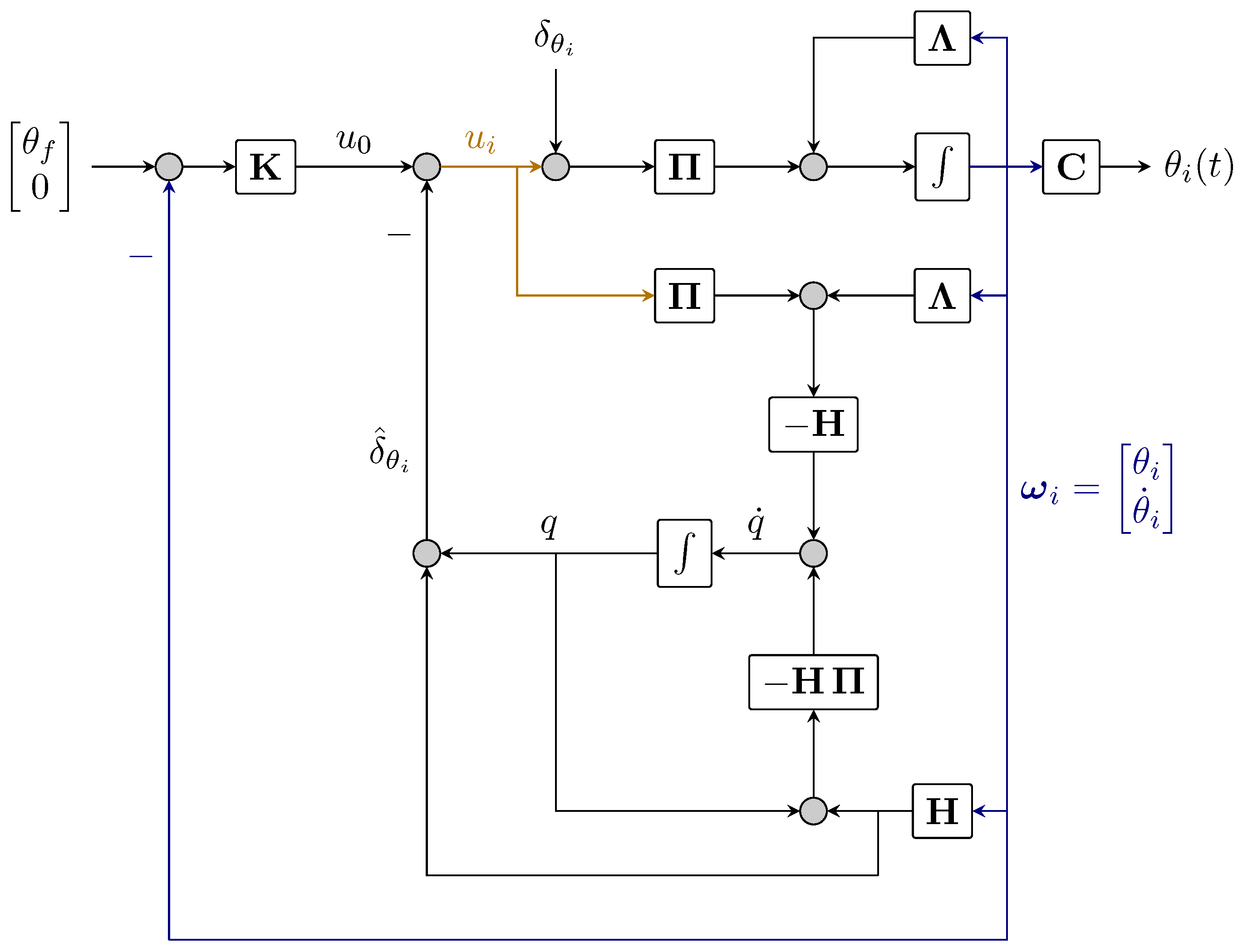
Law (27) is composed of a PD controller, coupled with a disturbance observer. Two reasons lead to this choice. First, PID controller could be used however we assume the disturbances to be time-varying, and PID is bad at rejecting time-varying disturbances [29]. Second, the controller used in [28] is also composed of a PD controller (considered as a nominal control) augmented by an ISC. This is purposely to make the comparison between controllers more fair and precise. As the disturbances are rejected, , the overall network depicts the desired patterns. As a remark, the form can be applied to any system with fixed gains. In [18], authors show that their network is also depicting epicycle and trochoid, and this formation relies on the eigenvalues of . Moreover, if the Laplacian is taken such that
where circ. stands for circular matrix [41]. The result would be the one presented in [19], as (26) is a special case of [22]. A representation of the used DOB is depicted in Figure 3.
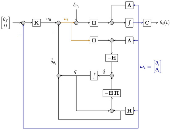
Figure 3.
Disturbance observer for agent i.
Disturbance rejection is also one of the main features of sliding mode control. This nonlinear control method alters the dynamics of a system by the application of high-frequency switching control. The state feedback control law switches from one continuous structure to another based on the current position in the state space. Hence, sliding mode control is a variable structure control method. The functioning and method of this controller applied to the network are as follows: Consider the system under (16) in the same conditions, where
where is a positive value, s is a sliding surface in which may be designed as a linear combination of the system dynamic angles, and z is designed to be seen as an integrator. The key difference with DOB lies in the design of (27a) which is expressed in terms of the sliding surface. As a result, the network (7) will possess imaginary axis eigenvalues and will keep its marginal stability despite uncertainties in the gains [28].
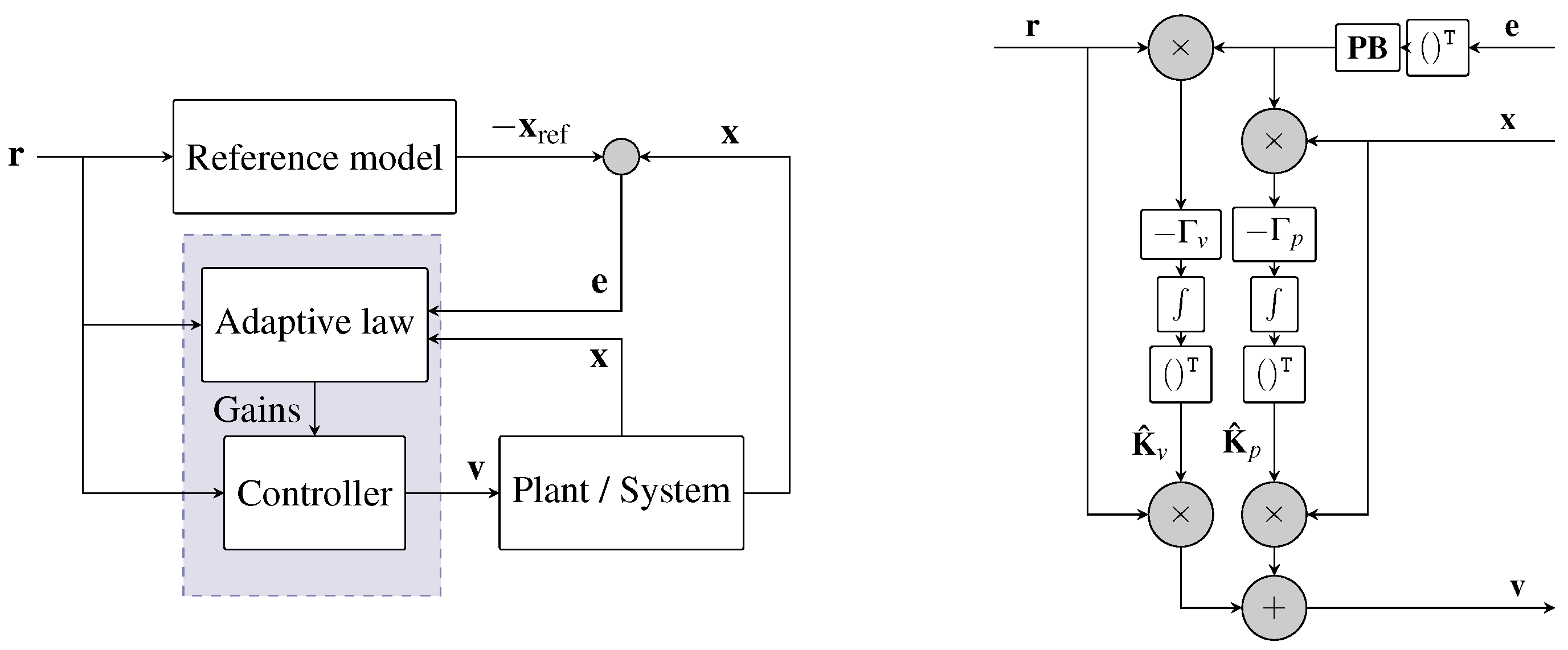
On the other hand, adaptive control can also be used to sustain the motion. We expand MRAC in [26] to the three-dimensional case and under the general topology pursuit. MRAC is an adaptive controller that uses the information it gathers during its closed-loop operation to change itself and improve its performance. The key difference between adaptive controllers and linear controllers is the adaptive controller’s ability to adjust itself to handle unknown model uncertainties. MRAC forces the output of the actual plant to tracks the output of a reference model having the same reference input. An uncertain plant, defined by
where and are uncertain matrices, needs to match a perfect model, defined by
where is a reference signal, through a proper choice of the control law . The block diagram is depicted in Figure 4.
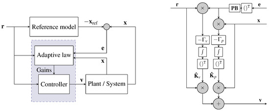
Figure 4.
(Left): General MRAC block diagram. (Right): Adaptive and control law details.
The method expanded here is to transform each agents’ control law to match the form of the MRAC one. Developing (5) for agent i, one can obtain
The main idea is to consider the leading agents’ positions as command signals and express (30) as
with
where is the position of agent i, is the state-reference matrix, is the reference control matrix, and is the sum of the positions of all neighboring agents of agent i. Straightforward analysis shows that is Hurwitz . Equations (31) and (32) represents the perfect behavior of each agent.
As explained, uncertainties can occur in (4) and the state-space equation for agent i is thus described by
where represents the model uncertainties, which are unknown but bounded. If uncertainties were known, the control law would be chosen in terms of fixed gains such that
Putting (34) into (33) gives
As (35) has to follow (31), one can obtain the matching conditions
that ensure perfect tracking.
Yet, as are unknown, the control fixed values law are replaced by their estimate
Putting (37) into (31)
the tracking error and its derivative can be expressed as
where
A Lyapunov analysis shows that, if the adaptive laws are chosen as
for a matrix satisfying the algebraic Lyapunov equation
for some , where the rates of adaptation and , then the closed-loop error dynamics are uniformly stable [26,39,42]. Henceforth, by ensuring the stability of the gains, the eigenvalues of the network will reach and stay at their desired location. In contrast to robust control techniques, under MRAC, uncertain plant parameters are directly identified and compensated instead of trying to find the best compromise between performance and robustness. To compare the effectiveness, some simulations have been conducted in the next section.
4. Simulations
Putting (46) into (16) gives the following numerical values
Equation (47a) is thus the value that each should tend to, despite the uncertainties. By selecting the axis of rotation associated with as
and by choosing the initial position vector as
the reference patterns as well as the eigenvalues repartition are shown in Figure 5.
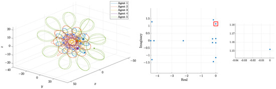
Figure 5.
Reference patterns and eigenvalues repartition.
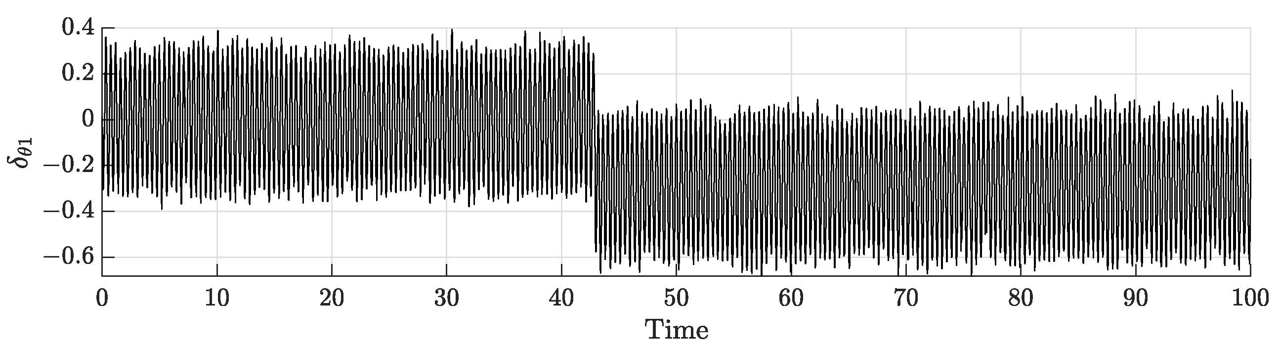
To analyze the efficiency of the controllers, the disturbances are selected to be
where , are constants proper to each agent, w is white noise, and is a step disturbance occurring at time . We chose the time of simulation as s. Uncertainties in are also taken into consideration. The numerical values are
| agent 1 | agent 2 | agent 3 | agent 4 | agent 5 | |
| −0.08 | 0.115 | 0.0275 | 0.11 | 0.0063 | |
| 14.8 | 25 | 17.8 | 26.8 | 17.4 | |
| (in percentage of ) | 42.92 | 26.32 | 14.7 | 79.60 | 18.93 |
| 3.0293 | 3.1808 | 3.0488 | 3.069 | 3.0128 | |
In the rest of the simulation, the obtained results will be traced only for agent 1 as the rest of the network is behaving in the same fashion. The uncertainties occurring on agent 1 gains are depicted in Figure 6.

Figure 6.
Uncertainties on agent 1 gains.
We also compare the results with the ISC using Equations (13), (14) and (24) from [28] under the same nominal control and disturbances as those of the DOB. To match the dimensions of the problem, we denote the gains for the nominal controller of the ISC and of the DOB as
We also select , and the following values for MRAC:
| agent 1 | agent 2 | agent 3 | agent 4 | agent 5 | |
| 5 | 4 | 9 | 3 | 1 | |
| 10 | 7.5 | 5 | 7 | 2 |
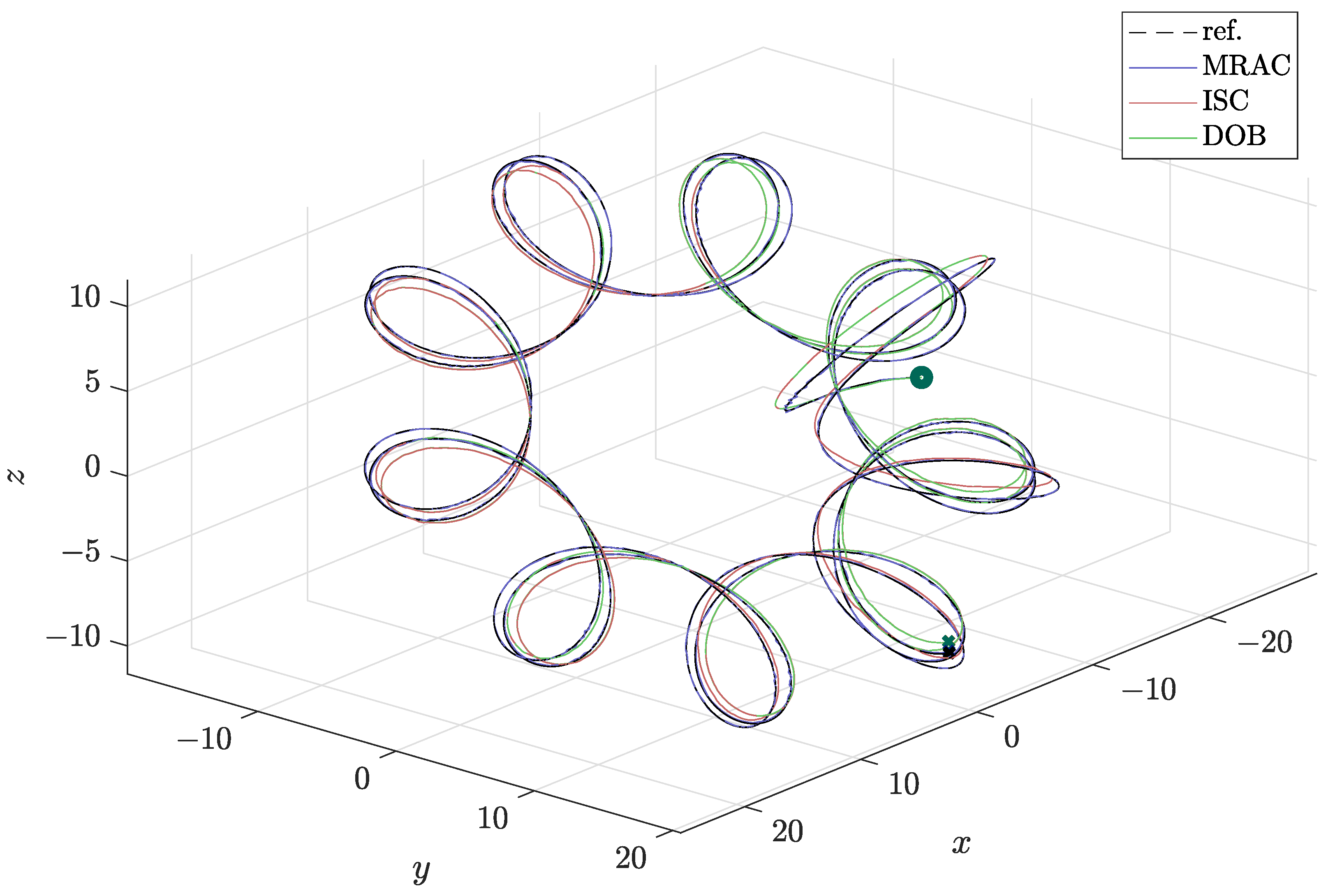
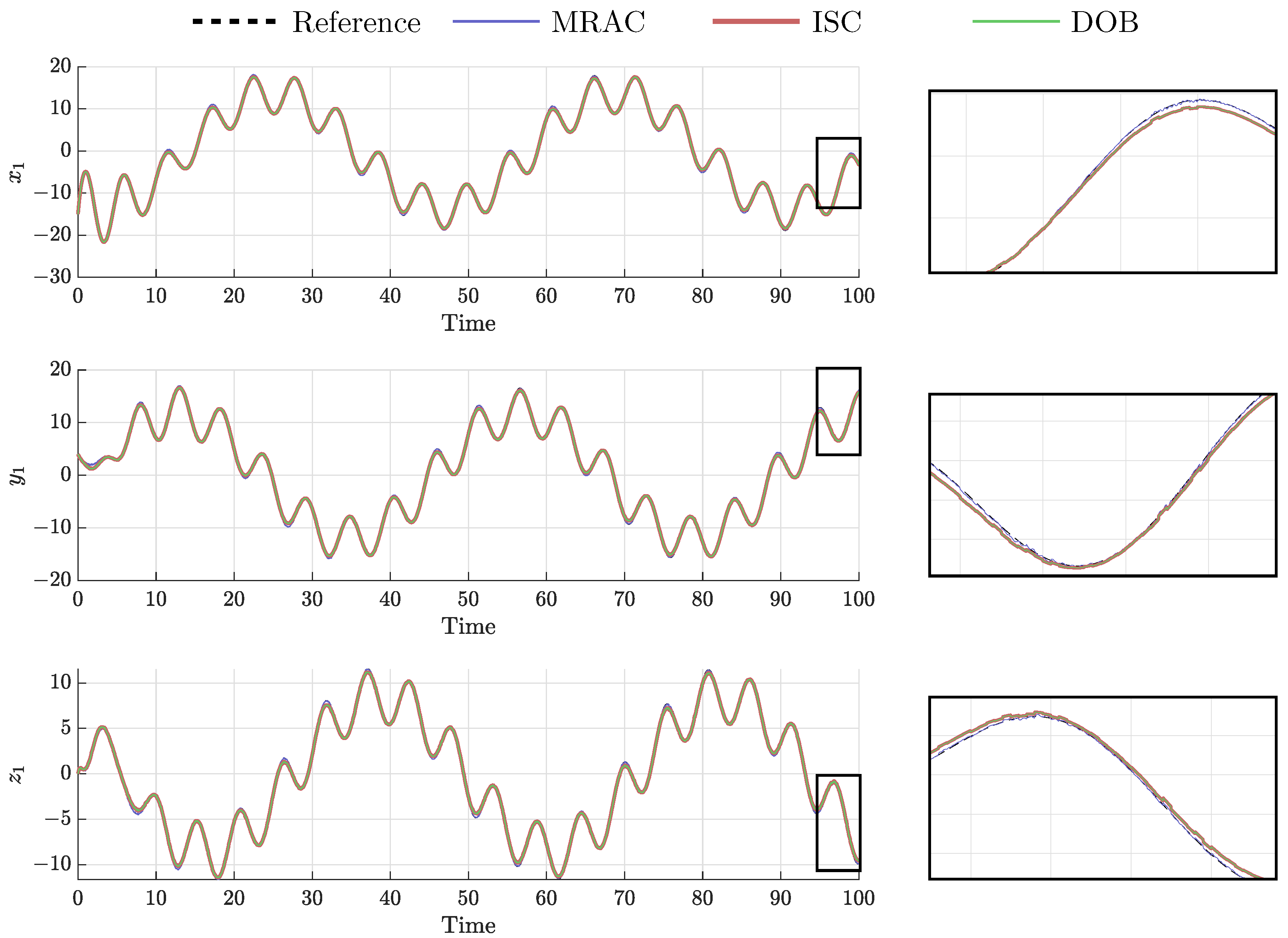
In order to compare the different controllers, the pattern of agent 1 is depicted in three dimensions in Figure 7 and the evolution of x, y, and z component are depicted in Figure 8.
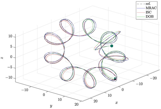
Figure 7.
Three-dimensional pattern of agent 1.
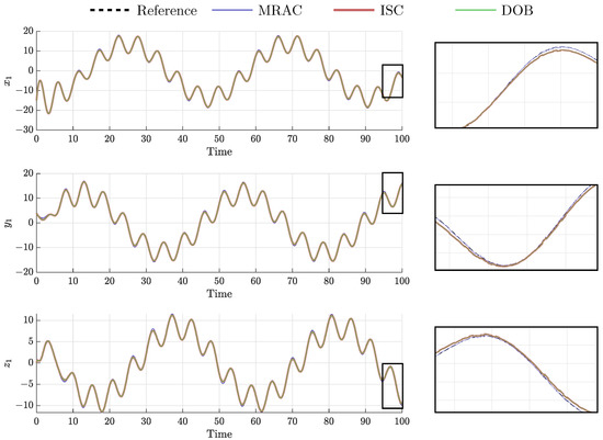
Figure 8.
Spatial component of agent 1’s pattern.
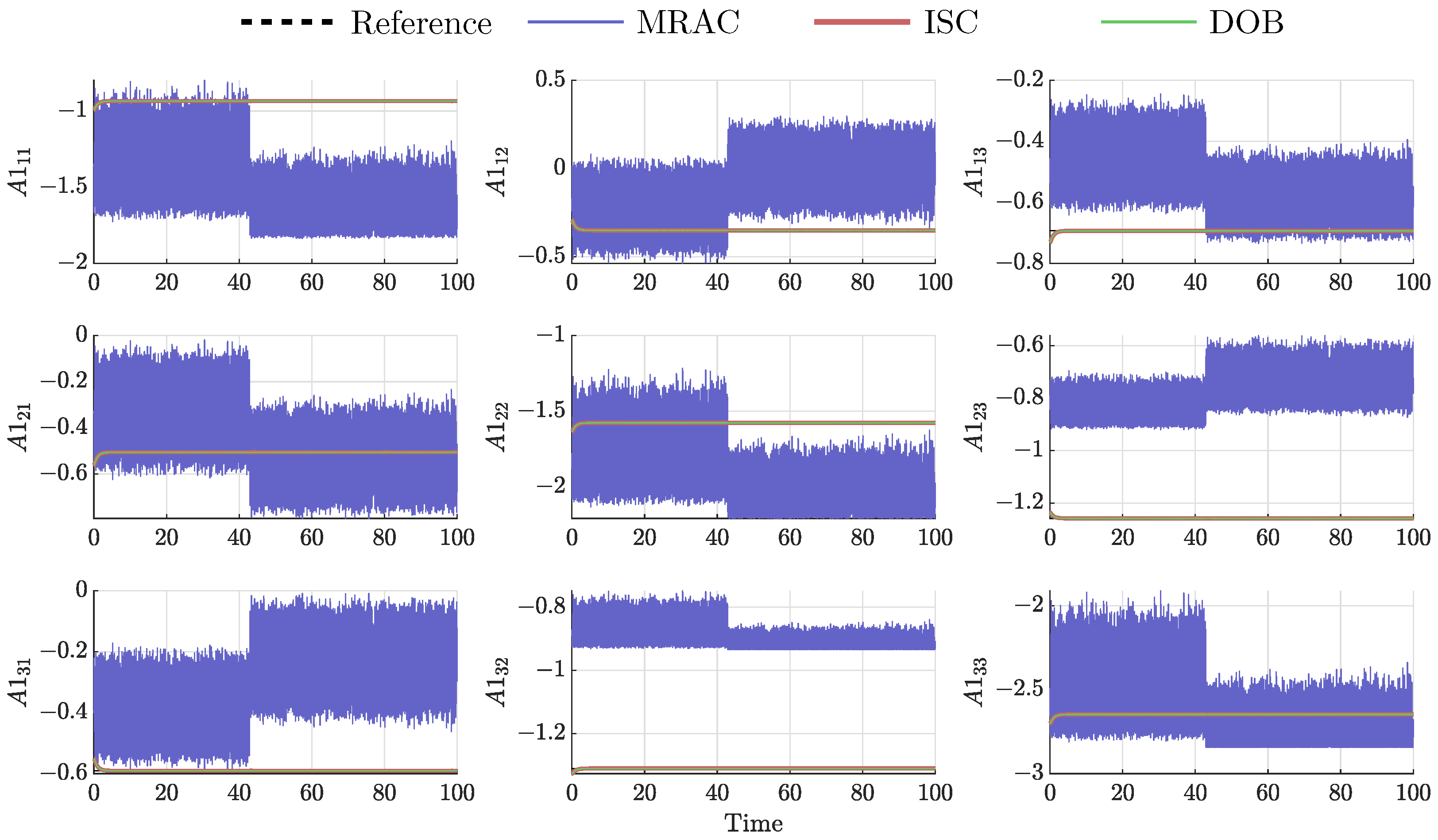
MRAC differs from the robust controllers in that it does not need previous knowledge of the bounds of uncertain or time-varying parameters; robust control guarantees that if the changes are within given bounds the control law need not be changed, while adaptive control is concerned with control law changing itself. It can be seen that the three controllers handle the uncertainties in their gains and show very satisfactory results. Every agent obeys the trajectory law (5), which, in its developed version, is a matrix for each agent. This matrix represents the gains’ evolution under uncertainties and correction. We denote for agent 1
As the focus is on the gains’ variation, their evolution is plotted for agent 1 in Figure 9.
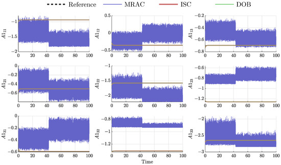
Figure 9.
Gains evolution of agent 1.
As seen, MRAC presents huge changes in the gains’ value, while ISC and DOB tend to a constant one. Therefore, MRAC presents very satisfactory result at a price of high-frequency change in the gains.
As they are robust controllers, DOB and ISC are compared for the rest of the experiment. As observed in Figure 8, the ISC and DOB present very similar results as their curves overlay. The main difference is found in the evolution of and in the control effort required, see Figure 10. It is observed that, under the same nominal controller, the ISC requires a larger control effort.
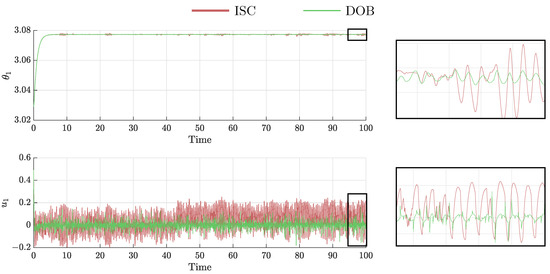
Figure 10.
(Top): Evolution of ; (Bottom): Control effort required.
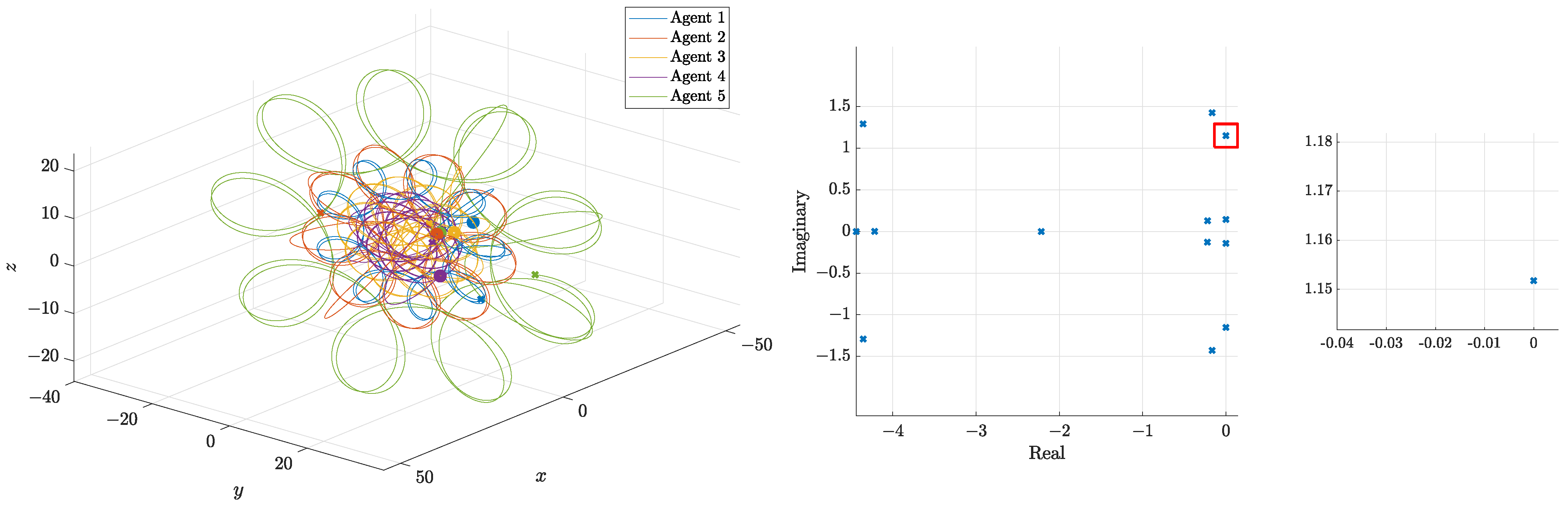
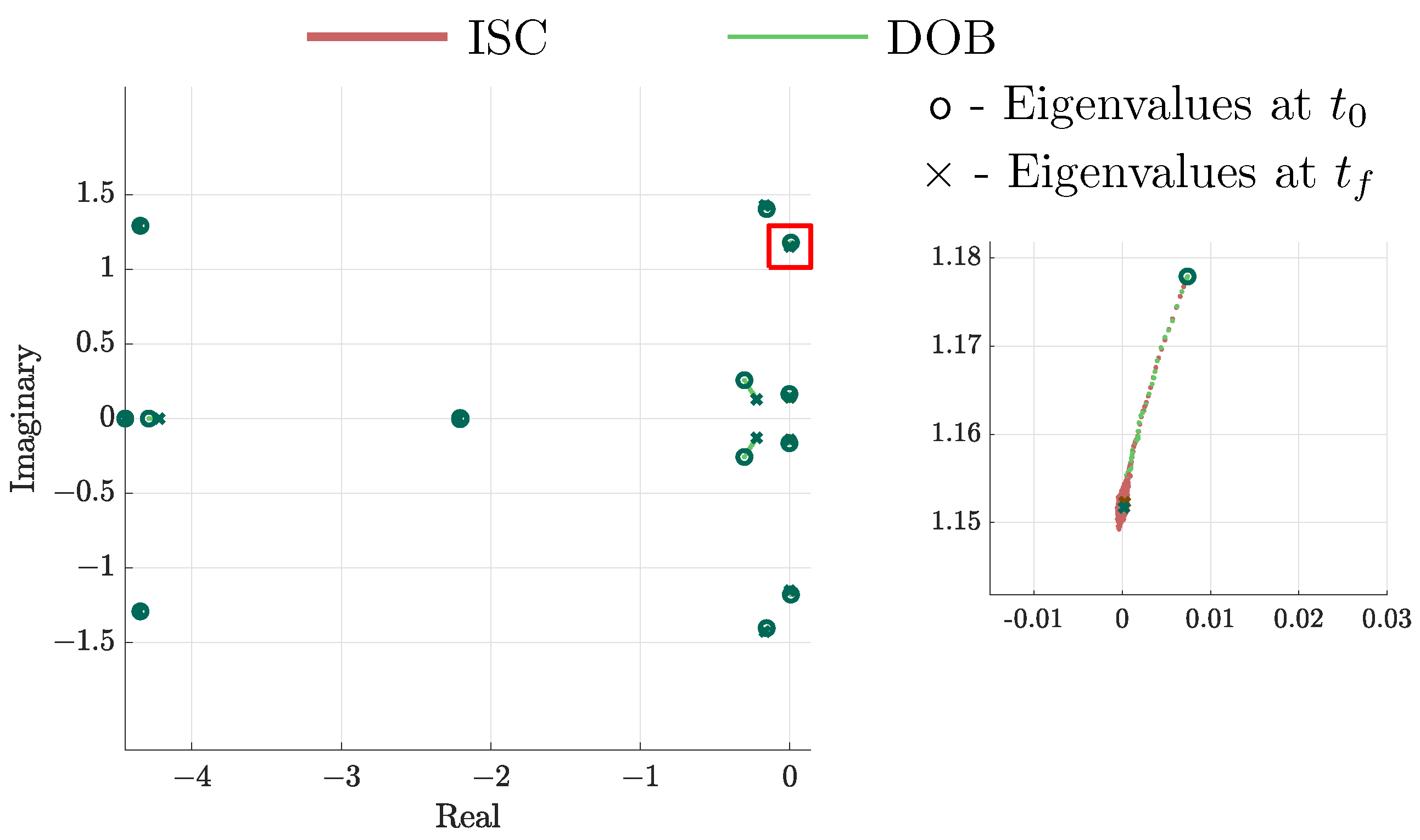
A final comparison is the evolution of the positions of the eigenvalues. As expected, both controllers bring the eigenvalues to their desired places, as seen in Figure 11; the circle marks the origin, while the cross marks the final position. It is clear that the eigenvalues reach the desired positions and maintain their designed values. As a result, the formation pattern is maintained despite uncertainties in the gains.
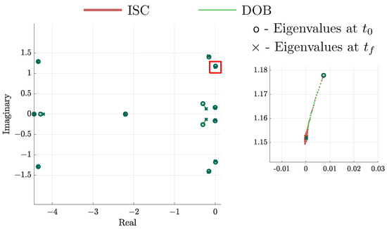
Figure 11.
Eigenvalues of agent 1 evolution under ISC and DOB.
It can be seen that the agent’s angles reach the desired final value with an acceptable control effort. Both robust controllers ensure the stability of the gains. The ISC has the cons of requiring a higher control effort, compared to the DOB. For the same nominal controller , it is a trade-off for the designer to chose between ISC and DOB. We can see that both controllers present very similar attitudes that evolve in the same manner.
Table 2 presents a quantitative comparison. As a precision, the control effort 1 is the highest, and the other values are expressed relatively, and the error is computed between the perfect position of agent i and its corrected position. The DOB controller presents the advantage of requiring less control effort than MRAC under the same disturbances and for similar performance (see Table 2); hence, DOB is a better choice. In conclusion, the MRAC controller presents excellent results in trajectory and formation maintenance, slightly better than agents under ISC or DOB. However, it induces a high-frequency change in the gains’ values. The agents under ISC or DOB present very similar results, the difference being in the control effort required, to which the DOB is lesser.
Table 2.
Quantitative comparison between the controllers.
5. Conclusions and Future Work
A group of n agents under general topology pursuit may exhibit a trochoid-like pattern. To do so, careful selection of their gains was previously designed, with the drawback of having a marginally stable network. In practice, it is desired to come up with a design that is robust against variations and disturbances. In the paper, previous methods using MRAC or ISC were reviewed, and the DOB scheme was developed. Comparisons between these three robust controllers for formation maintenance were made and trade-offs were analyzed. MRAC presents the best trajectory result but the highest control cost. ISC and DOB are robust controllers and present analogous results, DOB having the advantage of lesser control effort. By using these controllers, the formation is sustained in the presence of uncertainties.
However, there are some limitations as the model used is a single integrator, meaning that there are no physical constraints. Future research can include unicycle models or quadrotor models to be closer to reality. Moreover, this type of dynamic gains control can be applied to similar MAS with structurally unstable networks, e.g., to systems in [18].
Author Contributions
A.A. conceptualized and performed the experiments, analyzed the data, and wrote the manuscript. K.G.R. brought knowledge regarding graph theory, performed the experiments, and wrote the manuscript. J.-C.J. supervised the research, providing guidance theory, analyzed the data, and revised the paper. All authors have read and agreed to the published version of the manuscript.
Funding
The research is supported by the Ministry of Science and Technology (MOST), Taiwan, under grant MOST 109-2218-E-006-032.
Conflicts of Interest
The authors declare no conflict of interest.
Abbreviations
The following abbreviations are used in this manuscript:
| DOB(C) | Disturbance Observer (Control(ler)) |
| GCP | Generalized Cyclic Pursuit |
| GTP | Generalized Topology Pursuit |
| ISC | Integral Sliding (Mode) Control(ler) |
| MAS | Multi-Agent System(s) |
| MRAC | Model Reference Adaptive Control(ler) |
| PID | Proportional–Integral–Derivative (Control(ler)) |
Appendix A. Kronecker Product
The Kronecker product “⊗” is an operation on two matrices of arbitrary size resulting in a block matrix [43]. If is an matrix whose elements are and , and is a matrix, then the Kronecker product is the block matrix
Suppose that and are square matrices of size n and p, respectively. Let be the eigenvalues of , and be the eigenvalues of , then the eigenvalues of are
References
- Xiao, F.; Ligteringen, H.; Van Gulijk, C.; Ale, B. Nautical traffic simulation with multi-agent system for safety. In Proceedings of the 16th International IEEE Conference on Intelligent Transportation Systems (ITSC 2013), The Hague, The Netherlands, 6–9 October 2013; pp. 1245–1252. [Google Scholar]
- Dasgupta, P.; O’Hara, S.; Petrov, P. A multi-agent UAV swarm for automatic target recognition. In International Workshop on Defence Applications of Multi-Agent Systems; Springer: Berlin/Heidelberg, Germany, 2005; pp. 80–91. [Google Scholar]
- Abdelhameed, M.M.; Abdelaziz, M.; Hammad, S.; Shehata, O.M. Development and evaluation of a multi-agent autonomous vehicles intersection control system. In Proceedings of the 2014 International Conference on Engineering and Technology (ICET), Cairo, Egypt, 19–20 April 2014; pp. 1–6. [Google Scholar]
- Muylaert, J.; Reinhard, R.; Asma, C.; Buchlin, J.; Rambaud, P.; Vetrano, M. QB50, An International Network of 50 CubeSats for Multi-Point, In Situ Measurements in the Lower Thermosphere and Re-Entry Research. Available online: https://www.qb50.eu2012--2017 (accessed on 1 November 2011).
- Farrag, A.; Othman, S.; Mahmoud, T.; ELRaffiei, A.Y. Satellite swarm survey and new conceptual design for Earth observation applications. Egypt. J. Remote Sens. Space Sci. 2019, 24, 47–54. [Google Scholar] [CrossRef]
- Tan, Y. Handbook of Research on Design, Control, and Modeling of Swarm Robotics; IGI Global: Hershey, PA, USA, 2015. [Google Scholar] [CrossRef]
- Oh, K.K.; Park, M.C.; Ahn, H.S. A survey of multi-agent formation control. Automatica 2015, 53, 424–440. [Google Scholar] [CrossRef]
- Li, Y.; Tan, C. A survey of the consensus for multi-agent systems. Syst. Sci. Control Eng. 2019, 7, 468–482. [Google Scholar] [CrossRef] [Green Version]
- Tang, S.; Shinzaki, D.; Lowe, C.G.; Clark, C.M. Multi-Robot Control for Circumnavigation of Particle Distributions. In Distributed Autonomous Robotic Systems; Ani Hsieh, M., Chirikjian, G., Eds.; Springer: Berlin/Heidelberg, Germany, 2014; pp. 149–162. [Google Scholar]
- Mallik, G.; Sinha, A. Formation Control of Multi Agent System in Cyclic Pursuit with Varying Inter-Agent Distance. In Proceedings of the 1st Indian Control Conference, Chennai, India, 5–7 January 2015. [Google Scholar]
- Jin, L.; Yu, S.; Ren, D. Circular formation control of multiagent systems with any preset phase arrangement. J. Control Sci. Eng. 2018, 2018. [Google Scholar] [CrossRef] [Green Version]
- Briñón-Arranz, L.; Seuret, A.; Pascoal, A. Circular formation control for cooperative target tracking with limited information. J. Frankl. Inst. 2019, 356, 1771–1788. [Google Scholar] [CrossRef]
- Ghommam, J.; Saad, M.; Mnif, F. Finite-time circular formation around a moving target with multiple underactuated ODIN vehicles. Math. Comput. Simul. 2021, 180, 230–250. [Google Scholar] [CrossRef]
- Mischiati, M.; Krishnaprasad, P.S. Motion camouflage for coverage. In Proceedings of the 2010 American Control Conference, Baltimore, MD, USA, 30 June–2 July 2010; pp. 6429–6435. [Google Scholar] [CrossRef]
- Mischiati, M.; Krishnaprasad, P. Mutual motion camouflage in 3D. IFAC Proc. Vol. 2011, 44, 4483–4488. [Google Scholar] [CrossRef] [Green Version]
- DeVries, L.; Paley, D.A. Multivehicle control in a strong flowfield with application to hurricane sampling. J. Guid. Control Dyn. 2012, 35, 794–806. [Google Scholar] [CrossRef]
- Pavone, M.; Frazzoli, E. Decentralized Policies for Geometric Pattern Formation and Path Coverage. ASME J. Dyn. Syst. Meas. Control 2007, 129, 633–643. [Google Scholar] [CrossRef] [Green Version]
- Tsiotras, P.; Castro, L. Controls and Art; Chapter the Artistic Geometry of Consensus Protocols; Springer: Berlin/Heidelberg, Germany, 2014; pp. 129–153. [Google Scholar]
- Juang, J.C. On the Formation Patterns Under Generalized Cyclic Pursuit. IEEE Trans. Autom. Control 2013, 58, 2401–2405. [Google Scholar] [CrossRef]
- Juang, J.C. Cyclic pursuit control for dynamic coverage. In Proceedings of the 2014 IEEE Conference on Control Applications (CCA), Juan Les Antibes, France, 8–10 October 2014; pp. 2147–2152. [Google Scholar] [CrossRef]
- Jerome, M.M.; Sinha, A.; Boland, D. Geometric Pattern Formation on a Plane Under a General Graph Topology. IFAC PapersOnLine 2017, 50, 2391–2396. [Google Scholar] [CrossRef]
- Mose, J.M.; Sinha, A. Trochoidal patterns generation using generalized consensus strategy for single-integrator kinematic agents. Eur. J. Control 2019, 47, 84–92. [Google Scholar]
- DeLellis, P.; Garofalo, F. Novel decentralized adaptive strategies for the synchronization of complex networks. Automatica 2009, 45, 1312–1318. [Google Scholar] [CrossRef]
- Yu, W.; DeLellis, P.; Chen, G.; Di Bernardo, M.; Kurths, J. Distributed adaptive control of synchronization in complex networks. IEEE Trans. Autom. Control 2012, 57, 2153–2158. [Google Scholar] [CrossRef]
- Ding, W.; Yan, G.; Lin, Z. Pursuit formations with dynamic control gains. Int. J. Robust Nonlinear Control 2012, 22, 300–317. [Google Scholar] [CrossRef]
- Ansart, A.; Juang, J.C. Generalized Cyclic Pursuit: A Model-Reference Adaptive Control Approach. In Proceedings of the 2020 5th International Conference on Control and Robotics Engineering (ICCRE), Osaka, Japan, 24–26 April 2020; pp. 89–94. [Google Scholar] [CrossRef]
- Ansart, A.; Juang, J.C. Generalized Cyclic Pursuit: An Estimator-Based Model-Reference Adaptive Control Approach. In Proceedings of the 2020 28th Mediterranean Conference on Control and Automation (MED), Saint-Raphael, France, 15–18 September 2020; pp. 598–604. [Google Scholar] [CrossRef]
- Ansart, A.; Juang, J.C. Integral Sliding Control Approach for Generalized Cyclic Pursuit Formation Maintenance. Electronics 2021, 10, 1217. [Google Scholar] [CrossRef]
- Thien, R.T.; Kim, Y. Decentralized Formation Flight via PID and Integral Sliding Mode Control. IFAC PapersOnLine 2018, 51, 13–15. [Google Scholar] [CrossRef]
- Umeno, T.; Hori, Y. Robust speed control of DC servomotors using modern two degrees-of-freedom controller design. IEEE Trans. Ind. Electron. 1991, 38, 363–368. [Google Scholar] [CrossRef]
- Ohnishi, K.; Shibata, M.; Murakami, T. Motion control for advanced mechatronics. IEEE/ASME Trans. Mechatron. 1996, 1, 56–67. [Google Scholar] [CrossRef]
- Choi, Y.; Yang, K.; Chung, W.K.; Kim, H.R.; Suh, I.H. On the robustness and performance of disturbance observers for second-order systems. IEEE Trans. Autom. Control 2003, 48, 315–320. [Google Scholar] [CrossRef]
- Shim, H.; Jo, N.H. An almost necessary and sufficient condition for robust stability of closed-loop systems with disturbance observer. Automatica 2009, 45, 296–299. [Google Scholar] [CrossRef]
- Sariyildiz, E.; Oboe, R.; Ohnishi, K. Disturbance observer-based robust control and its applications: 35th anniversary overview. IEEE Trans. Ind. Electron. 2019, 67, 2042–2053. [Google Scholar] [CrossRef] [Green Version]
- Ha, S.W.; Park, B.S. Disturbance Observer-Based Control for Trajectory Tracking of a Quadrotor. Electronics 2020, 9, 1624. [Google Scholar] [CrossRef]
- Mesbahi, M.; Egerstedt, M. Graph Theoretic Methods in Multiagent Networks; Princeton University Press: Princeton, NJ, USA, 2010; Volume 33. [Google Scholar]
- Ren, W.; Beard, R. Consensus seeking in multiagent systems under dynamically changing interaction topologies. IEEE Trans. Autom. Control 2005, 50, 655–661. [Google Scholar] [CrossRef]
- Slotine, J.J.E.; Li, W. Applied Nonlinear Control; Prentice Hall: Englewood Cliffs, NJ, USA, 1991; Volume 199. [Google Scholar]
- Kersting, S.; Buss, M. Direct and Indirect Model Reference Adaptive Control for Multivariable Piecewise Affine Systems. IEEE Trans. Autom. Control 2017, 62, 5634–5649. [Google Scholar] [CrossRef]
- Chen, W.H.; Ballance, D.J.; Gawthrop, P.J.; O’Reilly, J. A nonlinear disturbance observer for robotic manipulators. IEEE Trans. Ind. Electron. 2000, 47, 932–938. [Google Scholar] [CrossRef] [Green Version]
- Davis, P.J. Circulant Matrices, 2nd ed.; American Mathematical Society: Providence, RI, USA, 1994. [Google Scholar]
- Eugene Lavretsky, K.A.W. Robust and Adaptive Control with Aerospace Applications; Springer: Berlin/Heidelberg, Germany, 2013. [Google Scholar]
- Graham, A. Kronecker Products and Matrix Calculus: With Applications; Ellis Horwood Limited: New York, NY, USA, 1981. [Google Scholar]

Publisher’s Note: MDPI stays neutral with regard to jurisdictional claims in published maps and institutional affiliations. |
© 2021 by the authors. Licensee MDPI, Basel, Switzerland. This article is an open access article distributed under the terms and conditions of the Creative Commons Attribution (CC BY) license (https://creativecommons.org/licenses/by/4.0/).