Trajectory Tracking and Stabilization of Nonholonomic Wheeled Mobile Robot Using Recursive Integral Backstepping Control

Abstract

In this paper, a generalized nontriangular normal form is presented to facilitate designing a recursive integral backstepping control for the class of underactuated nonholonomic systems, i.e., wheeled mobile robots (WMRs) that perform posture stabilization and trajectory tracking in environments without obstacles. Based on the differential geometry theory, we develop a multiple input multiple output (MINO) generalization of normal form using the input-output feedback linearization technique. Then, the change of variables (diffeomorphism) transform the state-space model of WMR, incorporating both kinematic and dynamic models into nontriangular normal form. As a result, the system dynamics can be represented as internal and external dynamics. The nonlinear internal dynamics of WMR pose serious challenges to design a suitable controller due to its internal dynamics being not minimum phase and non-strict feedback form structure. The proposed backstepping controller is designed in two steps. First, a standard integral backstepping controller is designed to stabilize the robot’s orientation angle. Then, a recursive integral backstepping control technique is applied to achieve asymptotic convergence of position error to zero. Hence, both asymptotic posture stabilization and trajectory tracking are achieved in semi-global regions, except the nonzero initial condition of the orientation angle. The asymptotic stability of the entire closed-loop system is shown using the Lyapunov criteria.

1. Introduction

Over the last decade, feedback control for the class of mechanical systems that possess both underactuated and nonholonomic behavior has gained remarkable interest among control researchers. Examples of these systems are wheeled mobile robot (WMR), legged robot, marine, and aerospace vehicles [1,2]. The control and stabilization of nonholonomic WMR are considered as one of the challenging benchmark problems due to their restricted mobility [3,4]. In an obstacle-free environment, motion planning and control tasks of WMR can be well defined as stabilization to an equilibrium point (posture stabilization) and stabilization to an equilibrium manifold (trajectory tracking) [5]. Conversely, posture stabilization for nonholonomic WMR is considered the most difficult task in comparison with trajectory tracking [6]. However, in [7], it was shown that the nonholonomic system does not satisfy Brockett’s necessary condition. As a result, any smooth state feedback control law cannot be applied to stabilize the WMR at the desired posture.

In the literature, various nonlinear control techniques have been suggested for posture stabilization that can be categorized into exact and dynamic feedback linearization [6,8], continuous time-varying feedback controller [9], and discontinuous feedback controller [10]. Similarly, for the trajectory tracking problem, various approaches have been presented, such as static and dynamic-based input-output feedback linearization [2,5,6,11,12,13,14,15,16,17,18,19], backstepping control [20,21,22,23,24,25,26], and sliding mode control [27].

Because of the peculiar nature and structural obstruction of the nonholonomic system, input-output feedback linearization has proved to be an effective and successful technique to control mobile robots [11,12,13,14,15,16,17,18]. The basic idea of this approach is to apply coordinates transformation to transform the overall system into nonlinear internal and linear external dynamics [28]. In these papers, the control law is designed to achieve only trajectory tracking without taking into account posture stabilization because the control law is only able to maneuver the external dynamics of the system. In contrast, the posture stabilization problem requires the asymptotic stabilization of a full closed-loop system, including both external and internal dynamics of WMR.

To date, some of the research papers have analyzed the stability of internal dynamics. In [16,17,18], the authors examined the behavior of internal dynamics of type (2,0) WMR using the dynamic model. They showed that the internal dynamics of WMR is stable but not asymptotically stable during the stabilization of the position vector. Furthermore, Ref. [5] observed the stability of internal dynamics of a car-like robot type (1,1) using the kinematic model. It showed that zero dynamics of tracking error is uniformly asymptotically stable under certain conditions. Moreover, Ref. [19] analyzed the internal dynamics of WMR during trajectory tracking and point stabilization with front-wheel steering and driving. They observed asymptotically stable internal dynamics during trajectory tracking provided that the steering angle is zero and the mobile robot moves forward and ultimately uniformly stable during point stabilization. It should be pointed out that three main reasons can be summarized that hinder the achievement of posture stabilization using the input-output feedback linearization approach: (1) The WMR can not be input-state linearizable by a smooth feedback control due to nonholonomic constraint [1,15], (2) internal dynamics of WMR are not minimum phase [1,16], and (3) the underactuated nonholonomic system (WMR) provides nontriangular normal form the structure [29]. Therefore, the internal dynamics of nonholonomic WMR are very complex and can not be feedback linearizable.

However, because of the above challenges, control of WMR necessitates advanced control techniques to achieve asymptotic stabilization of internal dynamics during both scenarios. In the recent literature, the backstepping approach has developed as an efficient design technique to control nonlinear systems. It is a Lyapunov-based design technique, which provides a recursive method that ensures the asymptotic stabilization of the entire system represented in strict-feedback form [21,28,30,31,32,33]. Conversely, many underactuated nonholonomic systems, including the state-space model or normal form structure [16,29], of WMR fail to obtain a strict feedback form. Therefore, to take the advantageous features of the integral backstepping design, many modified backstepping controllers have been presented in recent years [34,35,36,37].

In [22], a recursive backstepping approach is presented for the stabilization of a car-like robot, and [23] proposed the stabilization solution of the nonstationary motion of NWMR based on the backstepping technique. Similarly, trajectory tracking of a WMR using backstepping control is proposed by various researchers [3,24,25,38]. Nevertheless, the aforementioned techniques have proposed a solution either for tracking or stabilization, and as a result, most tracking controllers do not apply to the stabilization problems and require separate solutions for both problems. However, in a practical environment, trajectory tracking and stabilization are often performed simultaneously in one task, so it is better to implement a single controller that can handle both problems.

A single time-varying controller is designed to solve simultaneous stabilization and tracking problems using a kinematic model [39]. Another unified control for both problems based on dynamic feedback linearization using a kinematic model is presented in [6]. The results showed the exponential convergence of robot position $(x_0,y_0)$ to zero with an orientation angle stabilized to horizontal tangent ($\theta =0°$ or $\pi$), but having constrained on linear velocity to avoid the singularity. In [37], the authors presented a block-backstepping approach to achieve tracking and stabilization for a wheeled mobile robot. The proposed controller was further enhanced by incorporating integral action to improve steady-state performance but had a complex mathematical formulation and slow transient performance.

This paper proposes a generalized nontriangular normal form, as a special class of the Byrnes–Isidori normal form introduced in [40], to facilitate the recursive integral backstepping control for the class of MIMO underactuated nonholonomic system, i.e., WMR to solve trajectory tracking and posture stabilization. Based on the differential geometry theory, we develop a MIMO generalization of normal form using the input-output feedback linearization technique. Then, the change of variables (diffeomorphism) transform the dynamics of nonholonomic WMR into a nontriangular normal form. This normal form is distributed in two portions, internal and external dynamics. The nonlinear state feedback controller is applied to the external dynamics of the system and decouples the input-output map into two subsystems with a double-integrator linear part. Moreover, nonlinear internal dynamics will remain complicated and generally not feedback linearizable, as introduced in [40]. Afterward, the proposed backstepping controller will be designed in two steps. First, a standard integral backstepping controller is proposed to stabilize the robot’s orientation angle. Then, a recursive integral backstepping control technique is applied to achieve asymptotic convergence of position error to zero. This research work is noteworthy because it provides a solution for the stabilization and tracking of a large class of underactuated nonholonomic systems represented in nontriangular normal form. To our knowledge, trajectory tracking and posture stabilization based on a globally defined normal form using the backstepping technique has not been solved yet.

The main contributions of this research can be summarized as follows:

• We have proposed a novel generalized nontriangular normal form by a suitable change of coordinates (diffeomorphism) transformation. During the formulation of generalized nontriangular normal form, the output vector is selected in such a way that the decoupling matrix would be nonsingular, even when the look-ahead distance (coordinates of virtual reference point in front of the mobile robot) or linear velocity is zero, as compared with previous work [5,6,8,16,17,18,19]. The proposed internal dynamics of WMR is one dimension, where nonholonomic constraints of WMR has been sensibly exploited to reduce the complexity of nonlinear internal dynamics, with structural properties that provide ease to the design controller. In contrast to the previous research [16,18], internal dynamics were two-dimension coupling with the derivative of output functions.
• We have proposed a systematic method of ensuring asymptotic stabilization of internal dynamics during trajectory tracking and posture stabilization, unlike the previous research [16,17,18,19]. Furthermore, the proposed method used an exact model of nonlinear internal dynamics rather than a linear approximation of internal dynamics [5].
• This paper proposes a novel recursive integral backstepping control based on generalized nontriangular normal form structure for differential drive WMR. The proposed single controller can perform trajectory tracking and posture stabilization better than existing backstepping-based tracking/stabilization controllers [3,22,23,24,25,38]. Using a normal form representation of WMR makes the proposed algorithm simpler because of the features of regular backstepping technique as compared with modified backstepping control [20] and block-backstepping [37]. Moreover, the proposed controller provides a solution for the kinematic model cascaded with the dynamic model of WMR, as compared with previously designed controllers for kinematic and/or dynamics models [6,37,39]. In our approach, the actual robot motion commands are the wheel velocities rather than robot driving and steering velocities, calculated from the motor torques based on a dynamic model. Therefore, it would be more appropriate to represent the robot’s dynamic equations of motion based on wheel velocities to have a modular control structure unlike [37].

The outline of the remaining paper is organized as follows. Section 2 presents the stat-space model of WMR including both kinematic and dynamics models. The generalized nontriangular normal form of WMR using the input-output feedback linearization technique is presented in Section 3. The proposed backstepping controller for trajectory tracking is designed in Section 4. The proposed backstepping controller for posture stabilization is designed in Section 5. Section 6 illustrates the simulation results of the trajectory tracking and posture stabilization. Finally, Section 7 draws the conclusions.

2. Modeling of Nonholonomic WMR

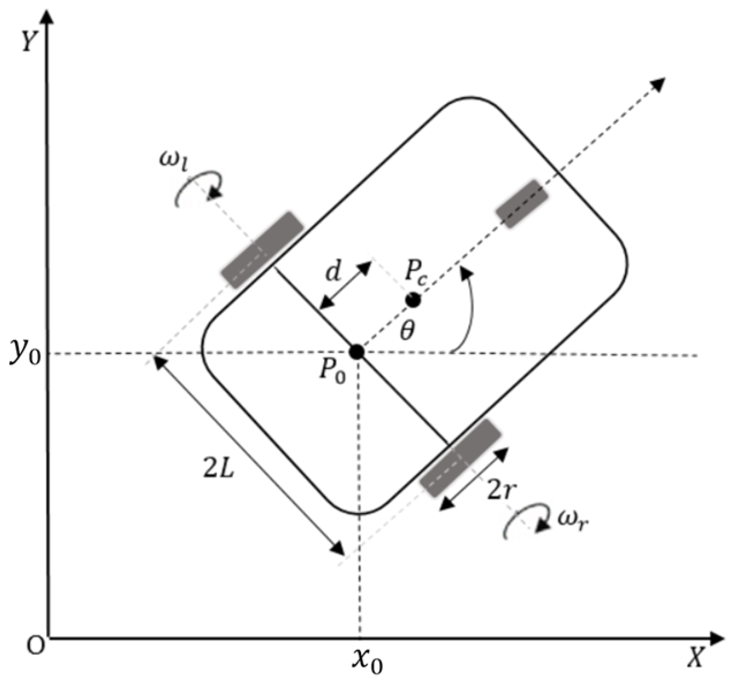
2.1. Kinematic Model of WMR

This section formulates the kinematic model of a differential drive wheeled mobile robot in Cartesian coordinates under nonholonomic constraints. The WMR represented in Figure 1 has two driving wheels on the same axis actuated by two independent motors providing torque to both right and left wheels. The radii of both wheels are indicated by r, which are separated by a distance of 2 L. The posture of WMR in the inertial Cartesian frame $\left\{O,X,Y\right\}$ can be describe by the position $(x_0,y_0)$, the coordinates of point $p_0$ and orientation angle $\theta$, measured with respect to the X-axis. The point $p_0$ defines the origin of the local coordinate frame, which is the intersection point of the driving wheel and axis of symmetry. The point $p_c$ denotes the center of the mass of mobile robot, which is d distance from point $p_0$.

Accordingly, the mobile robot in n-dimensional configuration space with n generalized coordinates $q={[x_0,y_0,\theta ]}^T,q\in R^n$, that is subject to m nonholonomic independent constraints can be describe as [11] (assuming that $m<n$):

$$A\left(q\right)\dot{q}=0$$

(1)

where $A\left(q\right)\in R^{m\ast n}$ is a full rank matrix linked with kinematic constraints. Assume a mobile robot satisfies the following nonholonomic constraint, i.e., two-wheel roll, and there is no lateral slip [27],

$$A\left(q\right)\dot{q}={\dot{x}}_0\sin \theta -{\dot{y}}_0\cos \theta =0$$

(2)

Let $S_1\left(q\right),\dots ..S_{n-m}\left(q\right)$ be linearly independent vector fields in the null space of A(q).

$$A\left(q\right)S\left(q\right)=0$$

(3)

The matrix S(q) can be defined as to verify the above condition

$$S\left(q\right)=\left[\begin{array}{cc}\cos \theta & 0\\ \sin \theta & 0\\ 0& 1\end{array}\right]$$

(4)

From Equations (2) and (3), it can be understood that constrained velocity will be in the null space of $A\left(q\right)$. So, it implores us to define velocity vector $\vartheta \left(t\right)\in R^{n-m}$ as such for all t.

$$\dot{q}=S\left(q\right)\vartheta \left(t\right)$$

(5)

The kinematic model of WMR under constraint condition can be defined as [6],

$$\dot{q}=\left[\begin{array}{c}{\dot{x}}_0\\ {\dot{y}}_0\\ \dot{\theta }\end{array}\right]=\left[\begin{array}{cc}\cos \theta & 0\\ \sin \theta & 0\\ 0& 1\end{array}\right]\left[\begin{array}{c}v\\ \omega \end{array}\right]$$

(6)

where v and $\omega$ can be defined as linear and angular velocities, respectively. The above model can be improved by transforming these velocities components into rotational velocities $({\omega }_r,{\omega }_l)$, provided by right and left wheel motor torque [21],

$$\left[\begin{array}{c}v\\ \omega \end{array}\right]=\frac{1}{2}\left[\begin{array}{cc}r& r\\ \frac{r}{L}& -\frac{r}{L}\end{array}\right]\left[\begin{array}{c}{\omega }_r\\ {\omega }_l\end{array}\right]$$

(7)

substituting Equation (7) into Equation (6), the more detailed kinematic model of WMR is formulated as:

$$\dot{q}=\left[\begin{array}{c}{\dot{x}}_0\\ {\dot{y}}_0\\ \dot{\theta }\end{array}\right]=S_k\left(q\right)\omega \left(t\right)=\underset{S_k\left(q\right)}{\underbrace{\left[\begin{array}{cc}a\cos \theta & a\cos \theta \\ a\sin \theta & a\sin \theta \\ b& -b\end{array}\right]}}\underset{\omega \left(t\right)}{\underbrace{\left[\begin{array}{c}{\omega }_r\\ {\omega }_l\end{array}\right]}}$$

(8)

where $a=\frac{r}{2},b=\frac{r}{2L}$.

2.2. Dynamic Model of WMR

The lagrange formulation will be used to drive the dynamic model of WMR given by [11],

$$M\left(q\right)\ddot{q}+C(q,\dot{q})\dot{q}=B\left(q\right)\tau -A^T\left(q\right)\lambda$$

(9)

where $M\left(q\right)\in R^{n\ast n}$ is a symmetric positive definite inertia matrix, $C(q,\dot{q})\in R^{n\ast n}$ represents the centripetal and coriolis fores, $B\left(q\right)\in R^{n\ast (n-m)}$ the input transformation matrix, $A\left(q\right)\in R^{m\ast n}$ constraints matrix, $\tau \in R^{n-m}$ the input torque vector, and $\lambda \in R^m$ the vector of constrain forces. These matrices can be defined as [14],

$$M\left(q\right)=\left[\begin{array}{ccc}m& 0& md\sin \theta \\ 0& m& -md\sin \theta \\ md\sin \theta & -md\cos \theta & I\end{array}\right],C(q,\dot{q})=\left[\begin{array}{ccc}0& 0& md\dot{\theta }\cos \theta \\ 0& 0& md\dot{\theta }\sin \theta \\ 0& 0& 0\end{array}\right]$$

$$B\left(q\right)=\frac{1}{r}\left[\begin{array}{cc}\cos \theta & \cos \theta \\ \sin \theta & \sin \theta \\ L& -L\end{array}\right],\tau ={\left[{\tau }_r{\tau }_l\right]}^T$$

where $m=m_c+2m_w,$ and $I=I_c+2I_m+m_c{d}^2+2m_w(L^2+d^2)$. $m_c$ is the mass of the robot platform, and $m_w$ is the mass of driving wheels with including rotors. $I_c$ is the moment of inertia of the mobile robot platform about a vertical axis through $p_c$. $I_m$ is the inertia of each wheel including the motor’s rotor about a wheel diameter.

2.3. State Space Model of WMR

The state-space model for a mobile robot can be developed by integrating the kinematic and dynamic model of the WMR to improvise the efficiency of the stabilizing and tracking controller. For the stabilization and tracking controller, the state-space model can be obtained by taking the time derivative of Equation (8), which gives:

$$\ddot{q}=\dot{S_k}\left(q\right)\omega \left(t\right)+S_k\left(q\right)\dot{\omega }\left(t\right)$$

(10)

Now, substituting Equations (8) and (10) into Equation (9) and then multiplying by $S_k^T$ and considering $S_k^T{A}^T\lambda =0$ because of Equation (3), we obtain

$$S_k^{T}M(\dot{S_k}\omega +S_k\dot{\omega })+S_k^{T}C\left(S_k\omega \right)=S_k^{T}B\tau$$

(11)

Simplifying the above Equation (11) for $\dot{\omega }$ gives,

$$\dot{\omega }=-{\overline{M}}^{-1}\overline{C}\omega +{\overline{M}}^{-1}\overline{B}\tau$$

(12)

where $\overline{M}=S_k^{T}M{S}_k,\overline{C}=S_k^{T}M\dot{S_k}+S_k^{T}C{S}_k,\overline{B}=S_k^{T}B$.

The state-space model of WMR based on Equations (8) and (12) is as follows:

$$\dot{x}=\left[\begin{array}{c}\dot{q}\\ \dot{\omega }\end{array}\right]=\left[\begin{array}{c}{\dot{x}}_0\\ {\dot{y}}_0\\ \dot{\theta }\\ {\dot{\omega }}_r\\ {\dot{\omega }}_l\end{array}\right]=\underset{f\left(x\right)}{\underbrace{\left[\begin{array}{c}{S}_k\omega \\ -{\overline{M}}^{-1}\overline{C}\omega \end{array}\right]}}+\underset{g\left(x\right)}{\underbrace{\left[\begin{array}{c}0\\ {\overline{M}}^{-1}\overline{B}\end{array}\right]}}\tau =f\left(x\right)+g\left(x\right)\tau$$

(13)

Hence, the matrices $\overline{M}$, $\overline{C}$, and $\overline{B}$ can be calculated as

$$\overline{M}=\left[\begin{array}{cc}{a}^{2}m+b^{2}I& a^{2}m-b^{2}I\\ a^{2}m-b^{2}I& a^{2}m+b^{2}I\end{array}\right],\overline{C}=\left[\begin{array}{cc}0& -2abdm\dot{\theta }\\ 2abdm\dot{\theta }& 0\end{array}\right],\overline{B}=\left[\begin{array}{cc}1& 0\\ 0& 1\end{array}\right]$$

Assumption 1.

Suppose the number of actuators inputs (r) satisfies the condition $(r\ge n-m)$, then the square matrix (${\overline{M}}^{-1}\overline{B}$) has full rank $(n-m)$.

Remark 1.

• The WMR (13) is not input-state feedback linearizable due to nonholonomic constraint, but it can be input-output feedback linearizable by choosing an appropriate output function [1,15].
• Input-output feedback linearization of WMR (13) cannot be achieved if the coordinates of point $p_0$, as shown in Figure 1, are selected as the output equation. To overcome this problem, either a new mathematical model is developed to a reference point $p_c$ or using the look-ahead control scheme [15].

Remark 2 (7, Theorem 1 (iii)). 

A Brockett’s necessary condition for the existence of a continuous state feedback law for Equation (13), which asymptotically stabilizes to $x_0\in R^{2n-m}$, is that the image of mapping $(x,\tau )$↦$\left(f\right(x)+g(x\left)\tau \right)$ contains a neighborhood of $0\in R^{2n-m}$ [41].

3. Input-Output Feedback Linearization: Normal form for WMR

In the literature, the input-output linearization technique is widely used for the application of trajectory tracking without taking into account posture stabilization. Due to its nonholonomic characteristics, the complicated nontriangular normal form structure of WMR makes it difficult to achieve asymptotic stabilization of internal dynamics. Conversely, the posture stabilization problem requires the asymptotic stabilization of an entire closed-loop system, including both external and internal dynamics of WMR. To overcome these challenges, an appropriate change of variables (diffeomorphism) by choosing a good output vector and internal dynamics variable allows us to develop a nontriangular normal form with structural properties, which can provide convenience to the design controller. This paper proposes the input-output feedback linearization approach in such a way that both posture stabilization and trajectory tracking can easily be implemented with the same output function. Since the system has two inputs, only a two-dimension output vector can be taken.

Proposition 1.

Consider that the multi-input nonlinear system (13) is partially input-output feedback linearizable with the following desired output vector $y\in R^{n-m}$,

$$\left[\begin{array}{c}{y}_1\\ y_2\end{array}\right]=\left[\begin{array}{c}{h}_1\left(x\right)\\ h_2\left(x\right)\end{array}\right]=\left[\begin{array}{c}\theta \\ x_0\cos \theta +y_0\sin \theta \end{array}\right]$$

(14)

Proof. 

Taking the Lie derivative of output (14), we obtain

$$\left[\begin{array}{c}{\dot{y}}_1\\ {\dot{y}}_2\end{array}\right]=\left[\begin{array}{c}{\dot{h}}_1\left(x\right)\\ {\dot{h}}_2\left(x\right)\end{array}\right]=\frac{\partial h}{\partial x}\dot{x}=L_{f}h\left(x\right)+L_{g}h\left(x\right)\tau =L_{f}h\left(x\right)$$

(15)

Similarly, rewriting the above equation yields

$$\begin{array}{cc}\hfill {\dot{y}}_1=& \dot{\theta }\hfill \\ \hfill {\dot{y}}_2=& {\dot{x}}_0\cos \theta +{\dot{y}}_0\sin \theta +(y_0\cos \theta -x_0\sin \theta )\dot{\theta }\hfill \end{array}$$

(16)

Substituting ${\dot{x}}_0,{\dot{y}}_0,$ and $\dot{\theta }$ from Equation (8) to Equation (16) results in

$$\left[\begin{array}{c}{\dot{y}}_1\\ {\dot{y}}_2\end{array}\right]=\underset{\phi \left(x\right)}{\underbrace{\left[\begin{array}{cc}b& -b\\ a-b(x_0\sin \theta -y_0\cos \theta )& a+b(x_0\sin \theta -y_0\cos \theta )\end{array}\right]}}\underset{\omega \left(t\right)}{\underbrace{\left[\begin{array}{c}{\omega }_r\\ {\omega }_l\end{array}\right]}}=\phi \left(x\right)\omega \left(t\right)$$

(17)

since $L_{g}h\left(x\right)\tau =0$ in Equation (15), we can take another derivative of Equation (17) until input $\tau$ appears

$$\ddot{y}=L_f^{2}h\left(x\right)+L_g{L}_{f}h\left(x\right)\tau =\dot{\phi }\left(x\right)\omega \left(t\right)+\phi \left(x\right)\dot{\omega }\left(t\right)$$

(18)

Substitute $\dot{\omega }$ from Equation (13) to the above equation, we have

$$\begin{array}{cc}\hfill \ddot{y}& =\dot{\phi }\omega +\phi (-{\overline{M}}^{-1}\overline{C}\omega +{\overline{M}}^{-1}\overline{B}\tau )\hfill \\ \hfill & =(\dot{\phi }\omega -\phi {\overline{M}}^{-1}\overline{C}\omega )+\left(\phi {\overline{M}}^{-1}\overline{B}\right)\tau =\alpha \left(x\right)+\beta \left(x\right)\tau \hfill \end{array}$$

(19)

where $\alpha \left(x\right)$ and $\beta \left(x\right)$ can be calculated as:

$$\begin{array}{cc}\hfill \alpha \left(x\right)=& \underset{\dot{\phi }\omega }{\underbrace{\left[\begin{array}{c}0\\ -{\dot{\theta }}^2(x_0\cos \theta +y_0\sin \theta )\end{array}\right]}}-\underset{\phi {\overline{M}}^{-1}\overline{C}\omega }{\underbrace{\left[\begin{array}{c}-{\gamma }_1({\omega }_r^2-{\omega }_l^2)\\ d{\dot{\theta }}^2+{\gamma }_1(x_0\sin \theta -y_0\cos \theta )({\omega }_r^2-{\omega }_l^2)\end{array}\right]}}\hfill \\ \hfill \beta \left(x\right)=& \underset{\phi {\overline{M}}^{-1}\overline{B}}{\underbrace{\left[\begin{array}{cc}{\gamma }_2& -{\gamma }_2\\ {\gamma }_3-{\gamma }_2(x_0\sin \theta -y_0\cos \theta )& {\gamma }_3+{\gamma }_2(x_0\sin \theta -y_0\cos \theta )\end{array}\right]}}\hfill \end{array}$$

(20)

and ${\gamma }_1=\frac{abdm}{I},{\gamma }_2=\frac{L}{rI},{\gamma }_3=\frac{1}{rm}$ are the physical parameters of WMR. After substituting $\alpha \left(x\right)$ and $\beta \left(x\right)$ into Equation (19), and the simplification of the resulting equation yields

$$\begin{array}{cc}\hfill \left[\begin{array}{c}{\ddot{y}}_1\\ {\ddot{y}}_2\end{array}\right]=& \left[\begin{array}{c}{\gamma }_1({\omega }_r^2-{\omega }_l^2)\\ -{\dot{\theta }}^2(x_0\cos \theta +y_0\sin \theta )-d{\dot{\theta }}^2-{\gamma }_1(x_0\sin \theta -y_0\cos \theta )({\omega }_r^2-{\omega }_l^2)\end{array}\right]\hfill \\ \hfill & +\left[\begin{array}{cc}{\gamma }_2& -{\gamma }_2\\ {\gamma }_3-{\gamma }_2(x_0\sin \theta -y_0\cos \theta )& {\gamma }_3+{\gamma }_2(x_0\sin \theta -y_0\cos \theta )\end{array}\right]\left[\begin{array}{c}{\tau }_r\\ {\tau }_l\end{array}\right]\hfill \end{array}$$

(21)

Therefore, the system (Equation(13)) has a relative degree four in $R^5$ (relative degree of each output is two). The necessary and sufficient requirement to check whether the system (13) is input-output feedback linearizable and decoupled with the proposed output (Equation (14)) is that det $\left(\beta \right(x\left)\right)\ne 0$.

$$det\left(\phi {\overline{M}}^{-1}\overline{B}\right)=\frac{2L}{r^{2}mI}$$

(22)

Hence, the determinant of $\beta \left(x\right)$ is nonsingular, the WMR (Equation (13)) is partially input-output feedback linearizable, with the nonlinear feedback control achieving input-output linearization and decoupling in the following form:

$$\tau =\beta {\left(x\right)}^{-1}(u-\alpha \left(x\right))$$

(23)

where u is an auxiliary control input.  □

Proposition 2.

Suppose there exists a globally defined change of variables given by

$$z=T\left(x\right)=\left[\begin{array}{c}\psi \left(x\right)\\ h_1\left(x\right)\\ L_f{h}_1\left(x\right)\\ h_2\left(x\right)\\ L_f{h}_2\left(x\right)\end{array}\right]\stackrel{\mathrm{def}}{=}\left[\begin{array}{c}\psi \left(x\right)\\ h_1\left(x\right)\\ {\dot{h}}_1\left(x\right)\\ h_2\left(x\right)\\ {\dot{h}}_2\left(x\right)\end{array}\right]\stackrel{\mathrm{def}}{=}\left[\begin{array}{c}\eta \\ {\xi }_1\\ {\xi }_2\\ {\xi }_3\\ {\xi }_4\end{array}\right]$$

(24)

that transform the dynamics of the system (Equation (13)) in the globally defined nontriangular normal form given by

$$\begin{array}{cc}\hfill \dot{\eta }& =\frac{\partial \psi }{\partial x}f\left(x\right)=f_0({\xi }_2,{\xi }_3)\hfill \\ \hfill {\dot{\xi }}_1& ={\xi }_2\hfill \\ \hfill {\dot{\xi }}_2& =L_f^2{h}_1\left(x\right)+L_g{L}_f{h}_1\left(x\right)\tau \hfill \\ \hfill {\dot{\xi }}_3& ={\xi }_4\hfill \\ \hfill {\dot{\xi }}_4& =L_f^2{h}_2\left(x\right)+L_g{L}_f{h}_2\left(x\right)\tau \hfill \end{array}$$

(25)

where $\psi \left(x\right)$ is chosen such that $T\left(x\right)$ in Equation (24) is a valid diffeomorphism on a domain $D_0\subset D$ in $R^5$ and satisfies the conditions:

$$\psi \left(0\right)=0 and \frac{\partial \psi }{\partial x}g\left(x\right)=0,\forall x\in D_0$$

(26)

Proof. 

It can be verified that, if we choose $\eta =\psi \left(x\right)=x_0\sin \theta -y_0\cos \theta$, it must satisfy the conditions in Equation (26) to obtain:

$$z=T\left(x\right)=\left[\begin{array}{c}{x}_0\sin \theta -y_0\cos \theta \\ \theta \\ b{\omega }_r-b{\omega }_l\\ x_0\cos \theta +y_0\sin \theta \\ a{\omega }_r+a{\omega }_l-(x_{0}sin\theta -y_{0}cos\theta )\dot{\theta }\end{array}\right]=\left[\begin{array}{c}\eta \\ {\xi }_1\\ {\xi }_2\\ {\xi }_3\\ {\xi }_4\end{array}\right]$$

(27)

the map $T\left(x\right)$ in Equation (27) will be diffeomorphism if and only if Jacobian matrix $\left[\begin{array}{c}\frac{\partial T}{\partial x}\end{array}\right]$ is nonsingular at a point $(x_0,y_0,\theta )\in D$, where D is domain of T.

$$\frac{\partial T}{\partial x}=\left[\begin{array}{ccccc}\sin \theta & -\cos \theta & x_0\cos \theta +y_0\sin \theta & 0& 0\\ 0& 0& 1& 0& 0\\ 0& 0& 0& b& -b\\ \cos \theta & \sin \theta & -x_0\sin \theta +y_0\cos \theta & 0& 0\\ -\dot{\theta }\sin \theta & \dot{\theta }\cos \theta & -(x_0\cos \theta +y_0\sin \theta )\dot{\theta }& a-b(x_0\sin \theta -y_0\cos \theta )& a+b(x_0\sin \theta -y_0\cos \theta )\end{array}\right]$$

It can be verified that $\frac{\partial T}{\partial x}$ has a full rank for all $x\in R^5$, so map $T\left(x\right)$ is global diffeomorphism. Clearly, $T\left(x\right)$ must be invertible, such that $x=T^{-1}$(z) for all $z\in T\left(D\right)$

$$\begin{array}{cc}\hfill x=& {\xi }_3\cos {\xi }_1+\eta \sin {\xi }_1\hfill \\ \hfill y=& \frac{({\xi }_3\cos {\xi }_1+\eta \sin {\xi }_1)\sin {\xi }_1-\eta }{\cos {\xi }_1}\hfill \\ \hfill \theta =& {\xi }_1\hfill \\ \hfill \left[\begin{array}{c}{\omega }_r\\ {\omega }_l\end{array}\right]=& {\left[\begin{array}{cc}b& -b\\ a-b\eta & a+b\eta \end{array}\right]}^{-1}\left[\begin{array}{c}{\xi }_2\\ {\xi }_4\end{array}\right]\hfill \end{array}$$

(28)

Now, the change of variables in Equation (27) will transform the system (Equation (13)) into the globally defined nontriangular normal form given by:

$$\begin{array}{cc}\hfill \dot{\eta }=& \dot{\theta }(x_0\cos \theta +y_0\sin \theta )={\xi }_2{\xi }_3\hfill \\ \hfill \dot{\xi }=& A_c\xi +B_c[\alpha \left(x\right)+\beta \left(x\right)\tau ]\hfill \\ \hfill y=& C_c\xi \hfill \end{array}$$

(29)

where $\xi \in R^4,\eta \in R^1$.

$$A_c=\left[\begin{array}{cccc}0& 1& 0& 0\\ 0& 0& 0& 0\\ 0& 0& 0& 1\\ 0& 0& 0& 0\end{array}\right],B_c=\left[\begin{array}{cc}0& 0\\ 1& 0\\ 0& 0\\ 0& 1\end{array}\right],C_c=\left[\begin{array}{cccc}1& 0& 0& 0\\ 0& 0& 1& 0\end{array}\right]$$

 □

This nontriangular normal form (Equation (29)) is divided into two parts, internal ($\eta$) and external ($\xi$) dynamics. The nonlinear feedback controller from Equation (23) will be applied to the external dynamics of the system and decouples the input-output map into two subsystems with a double-integrator linear part, while the nonlinear internal dynamics will remain complicated and generally is not feedback linearizable.

$$\begin{array}{cc}\hfill \dot{\eta }=& f_0({\xi }_2,{\xi }_3)={\xi }_2{\xi }_3\hfill \\ \hfill {\dot{\xi }}_1=& {\xi }_2\hfill \\ \hfill {\dot{\xi }}_2=& u_1\hfill \\ \hfill {\dot{\xi }}_3=& {\xi }_4\hfill \\ \hfill {\dot{\xi }}_4=& u_2\hfill \end{array}$$

(30)

Proposition 3.

The zero dynamics of $\dot{\eta }$ subsystems (Equation (30)) is not minimum phase.

$$\dot{\eta }=f_0(0,0)=0$$

Proof. 

The zero dynamics of the WMR (Equation (30)) can be obtained by setting ${\xi }_2={\xi }_3=0$ in $\dot{\eta }$ dynamics of above system, which results in

$$\dot{\eta }=0$$

it can be observed that zero dynamics of WMR is stable but not asymptotically stable. Hence, the internal dynamics is not minimum phase [28].  □

4. Backstepping Control Design for Trajectory Tracking

In this section, trajectory tracking control of WMR is presented using the backstepping approach to force the state trajectories of WMR (Equation (30)) to track a reference trajectory given by,

$$\begin{array}{cc}\hfill {\dot{\eta }}_r& ={\xi }_{2r}{\xi }_{3r}\hfill \\ \hfill {\dot{\xi }}_{1r}& ={\xi }_{2r}\hfill \\ \hfill {\dot{\xi }}_{2r}& =u_{1r}\hfill \\ \hfill {\dot{\xi }}_{3r}& ={\xi }_{4r}\hfill \\ \hfill {\dot{\xi }}_{4r}& =u_{2r}\hfill \end{array}$$

(31)

Now, tracking error can be formulated as:

$$\begin{array}{cc}\hfill {\eta }_e& =\eta -{\eta }_r\hfill \\ \hfill {\xi }_{ie}& ={\xi }_i-{\xi }_{ir}1\le i\le 4\hfill \end{array}$$

(32)

Taking the time derivative of error in Equation (32) gives us error dynamics of the trajectory tracking model:

$$\begin{array}{cc}\hfill {\Delta }_1& \left\{\begin{array}{c}\begin{array}{cc}\hfill {\dot{\xi }}_{1e}& ={\xi }_{2e}\hfill \\ \hfill {\dot{\xi }}_{2e}& =u_1-{\dot{\xi }}_{2r}\hfill \end{array}\end{array}\right.\hfill \end{array}$$

(33)

$$\begin{array}{cc}\hfill {\Delta }_2& \left\{\begin{array}{c}\begin{array}{cc}\hfill {\dot{\eta }}_e& =({\xi }_{2e}+{\xi }_{2r}){\xi }_{3e}+{\xi }_{2e}{\xi }_{3r}\hfill \\ \hfill {\dot{\xi }}_{3e}& ={\xi }_{4e}\hfill \\ \hfill {\dot{\xi }}_{4e}& =u_2-{\dot{\xi }}_{4r}\hfill \end{array}\end{array}\right.\hfill \end{array}$$

(34)

Assumption 2.

Assume ${\xi }_{ir}$ and its derivatives up to $i=1,\dots ,4,$ are all bounded for all $t\ge 0$ and ${\xi }_{ir}$, and its derivatives are available on-line.

However, to implement the backstepping control technique, the error dynamical equations are divided into two subsystems, where the ${\Delta }_1$ subsystem (Equation (33)) defines the error dynamics of orientation angle and the ${\Delta }_2$ subsystem (Equation (34)) describes the position error dynamics. Therefore, the proposed backstepping controller is designed in two steps. First, a standard integral backstepping controller is designed to stabilize the robot’s orientation angle. Then, a recursive integral backstepping control technique is applied to achieve asymptotic convergence of position error to zero.

Step 1: Stabilization of ${\Delta }_{\mathbf{1}}$ Subsystem

Proposition 4.

The error dynamics of orientation angle ${\xi }_{1e}$ in Equation (33) can be asymptotically stabilized by the state feedback control

$${\xi }_{2e}={\varphi }_1\left({\xi }_{1e}\right)=-k_1{\xi }_{1e}with{\varphi }_1\left(0\right)=0$$

(35)

where ${\xi }_{2e}$ is viewed as a virtual control input, and $k_1>0$.

Proof. 

Consider the Lyapunov candidate as $V_1\left({\xi }_{1e}\right)=\frac{1}{2}{\xi }_{1e}^2$, and it satisfies

$${\dot{V}}_1=-k_1{\xi }_{1e}^2$$

(36)

Hence, ${\dot{V}}_1$ is negative definite; therefore, the dynamics of ${\xi }_{1e}$ is asymptotically stable around the origin, i.e., ${\xi }_{1e}\to 0$ as $t\to \infty$.  □

To backstepping, we apply the change of variables $z_1={\xi }_{2e}-{\varphi }_1\left({\xi }_{1e}\right)={\xi }_{2e}+k_1{\xi }_{1e}$ to transform the dynamics of system (33) and (34) into the form

$$\begin{array}{cc}\hfill {\Delta }_1& \left\{\begin{array}{c}\begin{array}{cc}\hfill {\dot{\xi }}_{1e}& =-k_1{\xi }_{1e}+z_1\hfill \\ \hfill {\dot{z}}_1& =u_1-{\dot{\xi }}_{2r}-{\dot{\varphi }}_1\left({\xi }_{1e}\right)\hfill \end{array}\end{array}\right.\hfill \end{array}$$

(37)

$$\begin{array}{cc}\hfill {\Delta }_2& \left\{\begin{array}{c}\begin{array}{cc}\hfill {\dot{\eta }}_e& =({\xi }_{2r}-k_1{\xi }_{1e}){\xi }_{3e}-k_1{\xi }_{3r}{\xi }_{1e}+({\xi }_{3e}+{\xi }_{3r})z_1\hfill \\ \hfill {\dot{\xi }}_{3e}& ={\xi }_{4e}\hfill \\ \hfill {\dot{\xi }}_{4e}& =u_2-{\dot{\xi }}_{4r}\hfill \end{array}\end{array}\right.\hfill \end{array}$$

(38)

where ${\dot{\varphi }}_1\left({\xi }_{1e}\right)=\frac{\partial {\varphi }_1}{\partial {\xi }_{1e}}{\dot{\xi }}_{1e}=k_1^2{\xi }_{1e}-k_1{z}_1$.

Theorem 1.

The error dynamics of ${\Delta }_1$ subsystem (37) is asymptotically stable by the following state feedback control law

$$u_1=-{\xi }_{1e}+{\dot{\varphi }}_1+{\dot{\xi }}_{2r}-k_2{z}_1$$

(39)

where $k_2>0$.

Proof. 

Consider the Lyapunov function as

$$V_2({\xi }_{1e},z_1)=V_1+\frac{1}{2}{z}_1^2$$

(40)

The $\dot{V_2}$ along the trajectories of subsystem (37) gives

$${\dot{V}}_2=-k_1{\xi }_{1e}^2+z_1({\xi }_{1e}-{\dot{\varphi }}_1-{\dot{\xi }}_{2r}+u_1)$$

(41)

substituting the control law from Equation (39) into Equation (41), we obtain

$${\dot{V}}_2=-k_1{\xi }_{1e}^2-k_2{z}_1^2$$

(42)

Therefore, the origin of the ${\Delta }_1$ subsystem is asymptotically stable. Since ${\varphi }_1\left(0\right)=0$, then ${\xi }_{1e},{\xi }_{2e}\to 0$ as $t\to \infty$.  □

Step 2: Stabilization of ${\Delta }_{\mathbf{2}}$ Subsystem

Proposition 5.

The internal dynamics ${\eta }_e$ (Equation (38)) is asymptotically stabilizable using the following feedback control

$${\xi }_{3e}={\varphi }_2\left({\eta }_e\right)=-\frac{k_3{\eta }_e}{({\xi }_{2r}-k_1{\xi }_{1e})}with{\varphi }_2\left(0\right)=0,and{k}_3>0$$

(43)

Furthermore, the internal dynamics (Equation (38))

$$\begin{array}{cc}\hfill {\dot{\eta }}_e& =({\xi }_{2r}-k_1{\xi }_{1e}){\varphi }_2\left({\eta }_e\right)-\left(k_1{\xi }_{3r}\right){\xi }_{1e}+({\varphi }_2\left({\eta }_e\right)+{\xi }_{3r})z_1=F_1({\eta }_e,{\xi }_{1e},z_1)\hfill \end{array}$$

(44)

is input-to-state stable with respect to ${\xi }_{1e}$ and $z_1$, if the following condition is satisfied to avoid singularity, $\left|{\xi }_{2r}-k_1{\xi }_{1e}\right|$ = 0, for all $t⩾0$ in (Equation (43)),

C1. 

$∥{\xi }_{2r}\left(t\right)∥>k_1∥{\xi }_{1e}\left(t\right)∥$, for all $t⩾0$

Proof. 

Consider the Lyapunov function as $V_3\left({\eta }_e\right)=\frac{1}{2}{\eta }_e^2$. The derivative of $V_3$ along the trajectory of ${\eta }_e$ in (Equation (38)) is

$${\dot{V}}_3\left({\eta }_e\right)={\eta }_e[({\xi }_{2r}-k_1{\xi }_{1e}){\varphi }_2-\left(k_1{\xi }_{3r}\right){\xi }_{1e}+({\varphi }_2+{\xi }_{3r})z_1]$$

(45)

Now, substituting Equation (43) into Equation (45), it becomes

$$\begin{array}{cc}\hfill {\dot{V}}_3\left({\eta }_e\right)& ={\eta }_e[-k_3{\eta }_e-\left(k_1{\xi }_{3r}\right){\xi }_{1e}+({\varphi }_2+{\xi }_{3r})z_1]\hfill \end{array}$$

(46)

${\xi }_{1e},z_1$ converges to zero as $t\to \infty$, as shown in Theorem 1. Therefore, ${\xi }_{1e}=z_1\equiv 0$, Equation (46) reduces to, i.e., $F_1({\eta }_e,0,0)$

$${\dot{V}}_3\left({\eta }_e\right)=-k_3{\eta }_e^2$$

(47)

Since ${\dot{V}}_3\left({\eta }_e\right)$ is negative definite, ${\eta }_e$ remains bounded and converges to zero as $t\to \infty$, provided that the denominator term in Equation (43), $\left|{\xi }_{2r}-k_1{\xi }_{1e}\right|\ne 0$, for all $t⩾0$. To satisfy this condition, we simply require a suitable initialization of the reference trajectory ${\xi }_{2r}\left(0\right)$ and ${\xi }_{2e}\left(0\right)$. As condition C1. implies,

$$∥{\xi }_{2r}\left(0\right)∥>k_1∥{\xi }_{1e}\left(0\right)∥$$

(48)

This condition will preserve against singularity when the tracking error converges to zero during the initial transient. Hence, internal dynamics ${\eta }_e$ of system (38) is input-to-state stable, with ${\xi }_{1e}$ and $z_1$ as an input, and then ${\eta }_e$ dynamics of system (38) is uniformly asymptotically stable.  □

Now, the change of variable $z_2={\xi }_{3e}-{\varphi }_2\left({\eta }_e\right)$ transforms the dynamics of system (38) into new coordinates as:

$$\begin{array}{cc}\hfill {\Delta }_2& \left\{\begin{array}{c}\begin{array}{cc}\hfill {\dot{\eta }}_e& =-k_3{\eta }_e-k_1(z_2+{\xi }_{3r}){\xi }_{1e}+(z_2+{\varphi }_2+{\xi }_{3r})z_1+{\xi }_{2r}{z}_2=F_2({\eta }_e,z_2,{\xi }_{1e},z_1)\hfill \\ \hfill {\dot{z}}_2& ={\xi }_{4e}-{\dot{\varphi }}_2\hfill \\ \hfill {\dot{\xi }}_{4e}& =u_2-{\dot{\xi }}_{4r}\hfill \end{array}\end{array}\right.\hfill \end{array}$$

(49)

Proposition 6.

The error dynamics of ${\eta }_e$ and $z_2$ in subsystem (49) is asymptotically stable under the following state feedback control law

$${\xi }_{4e}={\varphi }_3({\eta }_e,z_2)=-{\eta }_e{\xi }_{2r}+{\dot{\varphi }}_2-k_4{z}_{2}with{\varphi }_3(0,0)=0$$

(50)

where ${\xi }_{4e}$ is viewed as a virtual control input, and $k_4$ is a positive scalar.

Proof. 

Let $V_4({\eta }_e,z_2)=V_3+\frac{1}{2}{z}_2^2$. Such that for $\dot{\eta }=F_2({\eta }_e,z_2,0,0)$, the derivative of $V_4({\eta }_e,z_2)$ along the trajectories of system (49) is

$${\dot{V}}_4=-k_3{\eta }_e^2+z_2({\eta }_e{\xi }_{2r}-{\dot{\varphi }}_2+{\xi }_{4e})$$

(51)

Now, substitute Equation (50) into Equation (51), which will produce

$${\dot{V}}_4=-k_3{\eta }_e^2-k_4{z}_2^2$$

(52)

Hence, ${\dot{V}}_4$ is negative definite; therefore, ${\eta }_e$ and $z_2$ remains bounded and exponentially converges to zero as $t\to \infty$.  □

Now, the change of variable $z_3={\xi }_{4e}-{\varphi }_3({\eta }_e,z_2)$ transforms system (49) into

$$\begin{array}{cc}\hfill {\Delta }_2& \left\{\begin{array}{c}\begin{array}{cc}\hfill {\dot{\eta }}_e& =-k_3{\eta }_e-k_1(z_2+{\xi }_{3r}){\xi }_{1e}+(z_2+{\varphi }_2+{\xi }_{3r})z_1+{\xi }_{2r}{z}_2\hfill \\ \hfill {\dot{z}}_2& =-k_4{z}_2-{\eta }_e{\xi }_{2r}+z_3\hfill \\ \hfill {\dot{z}}_3& =u_2-{\dot{\xi }}_{4r}-{\dot{\varphi }}_3({\eta }_e,z_2)\hfill \end{array}\end{array}\right.\hfill \end{array}$$

(53)

Theorem 2.

Consider the ${\Delta }_2$ subsystem (Equation (53)), the following state feedback control law

$$u_2=-k_5{z}_3-z_2+{\dot{\xi }}_{4r}+{\dot{\varphi }}_3$$

(54)

asymptotically stabilizes the ${\Delta }_2$ subsystem (Equation (53)).

Proof. 

Consider a composite Lyapunov function $V_5({\eta }_e,z_2,z_3)=V_4+\frac{1}{2}{z}_3^2$.

The time derivative of $V_5$ along the trajectories of system (53), we obtained

$${\dot{V}}_5=-k_3{\eta }_e^2-k_4{z}_2^2+(z_2-{\dot{\xi }}_{4r}-{\dot{\varphi }}_3+u_2)z_3$$

(55)

substituting control law $u_2$ from Equation (54) into Equation (55), which yields

$${\dot{V}}_5=-k_3{\eta }_e^2-k_4{z}_2^2-k_5{z}_3^2$$

(56)

Hence, the origin of the ${\Delta }_2$ subsystem is asymptotically stable. Since ${\varphi }_2\left(0\right),{\varphi }_3(0,0)=0$, ${\eta }_e,{\xi }_{3e},{\xi }_{4e}\to 0$ as $t\to \infty$.  □

The solution of control law $u_1$ (Equation (39)) can be expressed in original coordinates as

$$u_1=-(1+k_1{k}_2)(\theta -{\theta }_r)-(k_1+k_2)(\dot{\theta }-{\dot{\theta }}_r)+{\ddot{\theta }}_r$$

(57)

Similarly, the control law $u_2$ (Equation (54)) can be expressed in original coordinates after calculating ${\dot{\varphi }}_2$ and ${\dot{\varphi }}_3$. where ${\dot{\varphi }}_2\left({\eta }_e\right)=\frac{\partial {\varphi }_2}{\partial {\eta }_e}{\dot{\eta }}_e=-\frac{k_3}{{\xi }_{2r}-k_1{\xi }_{1e}}{\dot{\eta }}_e$ and ${\dot{\varphi }}_3({\eta }_e,z_2)=\frac{\partial {\varphi }_3}{\partial {\eta }_e}{\dot{\eta }}_e+\frac{\partial {\varphi }_3}{\partial z_2}{\dot{z}}_2=-({\xi }_{2r}+\frac{k_3{k}_4}{{\xi }_{2r}-k_1{\xi }_{1e}}){\dot{\eta }}_e-k_4{\dot{z}}_2$

Now, substituting $z_2,z_3,{\dot{\varphi }}_2,{\dot{\varphi }}_3$ into Equation (54) yields

$$\begin{array}{cc}\hfill u_2=& -(k_5{\dot{h}}_{1r}+\frac{k_3{k}_4{k}_5}{D}+\frac{k_3}{D})(\eta -{\eta }_r)-(k_4{k}_5+1)(h_2-h_{2r})-(k_4+k_5)({\dot{h}}_2-{\dot{h}}_{2r})\hfill \\ \hfill & -(\frac{k_3{k}_5}{D}+{\dot{h}}_{1r}+\frac{2k_3{k}_4}{D})[{\dot{h}}_1(h_2-h_{2r})+({\dot{h}}_1-{\dot{h}}_{1r})+h_{2r}]+{\ddot{h}}_{2r}\hfill \end{array}$$

(58)

where $D={\dot{h}}_{1r}-k_1(h_1-h_{1r})$

5. Backstepping Control Design for Posture Stabilization

Consider systems (33) and (34), by setting all reference signals to zero, it can be rewritten in the following form

$$\begin{array}{cc}\hfill {\Delta }_1& \left\{\begin{array}{c}\begin{array}{cc}\hfill {\dot{\xi }}_1& ={\xi }_2\hfill \\ \hfill {\dot{\xi }}_2& =u_1\hfill \end{array}\end{array}\right.\hfill \end{array}$$

(59)

$$\begin{array}{cc}\hfill {\Delta }_2& \left\{\begin{array}{c}\begin{array}{cc}\hfill \dot{\eta }& ={\xi }_2{\xi }_3\hfill \\ \hfill {\dot{\xi }}_3& ={\xi }_4\hfill \\ \hfill {\dot{\xi }}_4& =u_2\hfill \end{array}\end{array}\right.\hfill \end{array}$$

(60)

Using the same virtual state feedback control, formulated in Equations (35), (43), and (50) by setting all reference signals to zero, yields:

$$\begin{array}{cc}\hfill {\xi }_2& ={\varphi }_1\left({\xi }_1\right)=-k_1{\xi }_1\hfill \end{array}$$

(61)

$$\begin{array}{cc}\hfill {\xi }_3& ={\varphi }_2\left(\eta \right)=\frac{k_3\eta }{k_1{\xi }_1}\hfill \end{array}$$

(62)

$$\begin{array}{cc}\hfill {\xi }_4& ={\varphi }_3(\eta ,z_2)={\dot{\varphi }}_2-k_4{z}_2\hfill \end{array}$$

(63)

Similarly, with the change of variables,

$$\begin{array}{cc}\hfill z_1& ={\xi }_2-{\varphi }_1\left({\xi }_1\right)\hfill \end{array}$$

(64)

$$\begin{array}{cc}\hfill z_2& ={\xi }_3-{\varphi }_2\left(\eta \right)\hfill \end{array}$$

(65)

$$\begin{array}{cc}\hfill z_3& ={\xi }_4-{\varphi }_3(\eta ,z_2)\hfill \end{array}$$

(66)

transform the dynamics of system (59) and (60) into the form

$$\begin{array}{cc}\hfill {\Delta }_1& \left\{\begin{array}{c}\begin{array}{cc}\hfill {\dot{\xi }}_1& =-k_1{\xi }_1+z_1\hfill \\ \hfill {\dot{z}}_1& =u_1-{\dot{\varphi }}_1\left({\xi }_1\right)\hfill \end{array}\end{array}\right.\hfill \end{array}$$

(67)

$$\begin{array}{cc}\hfill {\Delta }_2& \left\{\begin{array}{c}\begin{array}{cc}\hfill \dot{\eta }& =-k_3\eta -\left(k_1{z}_2\right){\xi }_1+(z_2+{\varphi }_2)z_1\hfill \\ \hfill {\dot{z}}_2& =-k_4{z}_2+z_3\hfill \\ \hfill {\dot{z}}_3& =u_2-{\dot{\varphi }}_3(\eta ,z_2)\hfill \end{array}\end{array}\right.\hfill \end{array}$$

(68)

Theorem 3.

Consider systems (67)–(68). Setting ${\xi }_{1r}={\xi }_{2r}={\xi }_{3r}={\xi }_{4r}=0$ in state feedback control law (39) and (54), i.e., choosing

$$\begin{array}{cc}\hfill u_1& =-{\xi }_1+{\dot{\varphi }}_1-k_2{z}_1\hfill \\ \hfill u_2& =-k_5{z}_3-z_2-{\dot{\varphi }}_3\hfill \end{array}$$

(69)

yields exponential convergence of systems (67)–(68) to originate from any initial configuration belonging to the set $\mathsf{\Omega }=\left\{{(\eta \left(0\right),{\xi }_1\left(0\right),z_1\left(0\right),z_2\left(0\right),z_3\left(0\right))}^T\in R^5/{\xi }_1\left(0\right)\ne 0\right\}$, if the following conditions are satisfied to ensure a bounded solution of Equation (62), which has directly linked with the stability of internal dynamics η in Equation (60),

C1. 

${(k_1+k_2)}^2-4(1+k_1{k}_2)>0$

C2. 

$∥{\xi }_1\left(t\right)∥\ne 0$ for all $t⩾0$

Proof. 

We break up the proof in two steps. In a first step, we show that Equation (62) will remain bounded as ${\xi }_1\left(t\right)$ converges to the origin. In the second step, we prove that the dynamics of systems (67)–(68) exponentially converge to origin under state feedback control (Equation (69)). (i) The solution of subsystem (59) can be obtained under state feedback control law $u_1$ (69) expressed in original coordinates $({\xi }_1=\theta$, ${\xi }_2=\dot{\theta })$ as

$$\begin{array}{cc}\hfill {\Delta }_1& \left\{\begin{array}{c}\begin{array}{cc}\hfill {\dot{\xi }}_1& ={\xi }_2\hfill \\ \hfill {\dot{\xi }}_2& =-(1+k_1{k}_2){\xi }_1-(k_1+k_2){\xi }_2\hfill \end{array}\end{array}\right.\hfill \end{array}$$

(70)

The solution of the above equations ${\xi }_1\left(t\right)$ and ${\xi }_2\left(t\right)$ can be written as

$$\left[\begin{array}{c}{\xi }_1\left(t\right)\\ {\xi }_2\left(t\right)\end{array}\right]=e^{At}\left[\begin{array}{c}{\xi }_1\left(0\right)\\ {\xi }_2\left(0\right)\end{array}\right]$$

(71)

where

$$e^{At}=\left[\begin{array}{cc}-\frac{(k_1+k_2-{\lambda }_1)}{({\lambda }_1-{\lambda }_2)}{e}^{-{\lambda }_1\left(t\right)}+\frac{(k_1+k_2-{\lambda }_2)}{({\lambda }_1-{\lambda }_2)}{e}^{-{\lambda }_2\left(t\right)}& -\frac{1}{({\lambda }_1-{\lambda }_2)}{e}^{-{\lambda }_1\left(t\right)}+\frac{1}{({\lambda }_1-{\lambda }_2)}{e}^{-{\lambda }_2\left(t\right)}\\ \\ \frac{(1+k_1{k}_2)}{({\lambda }_1-{\lambda }_2)}{e}^{-{\lambda }_1\left(t\right)}-\frac{(1+k_1{k}_2)}{({\lambda }_1-{\lambda }_2)}{e}^{-{\lambda }_2\left(t\right)}& \frac{{\lambda }_1}{({\lambda }_1-{\lambda }_2)}{e}^{-{\lambda }_1\left(t\right)}-\frac{{\lambda }_2}{({\lambda }_1-{\lambda }_2)}{e}^{-{\lambda }_2\left(t\right)}\end{array}\right]$$

and

$${\lambda }_{1,2}=\frac{(k_1+k_2)\pm \sqrt{{(k_1+k_2)}^2-4(1+k_1{k}_2)}}{2}$$

Since condition C1. ensures that the eigenvalues are real, trajectories of both ${\xi }_1$ and ${\xi }_2$ never cross zero (origin). Similarly, with the choice of initial condition, ${\xi }_1\left(0\right)\ne 0$ will avoid singularity during the initial transient in Equation (62) under the condition C2. Hence, we can say that ${\xi }_1\left(t\right)\ne 0$ for all $t⩾0$. Now, the dynamics of $\dot{\eta }$ can be rewritten after substituting Equations (61) and (62) into Equation (60) as

$$\dot{\eta }=(-k_1{\xi }_1)\frac{k_3\eta }{k_1{\xi }_1}=-k_3\eta$$

(72)

(ii) Consider a composite Lyapunov function $V_{c1}({\xi }_1,z_1)=\frac{1}{2}{\xi }_1^2+\frac{1}{2}{z}_1^2$ and $V_{c2}(\eta ,z_2,z_3)=\frac{1}{2}{\eta }^2+\frac{1}{2}{z}_2^2+\frac{1}{2}{z}_3^2$ for the two subsystems (67) and (68), respectively.

$$V=V_{c1}({\xi }_1,z_1)+V_{c2}(\eta ,z_2,z_3)$$

(73)

Since $\dot{V}$ is negative definite along the trajectories of closed-loop systems (67) and (68). Hence, the origin of closed-loop systems (67) and (68) is asymptotically stable.  □

6. Simulation Results

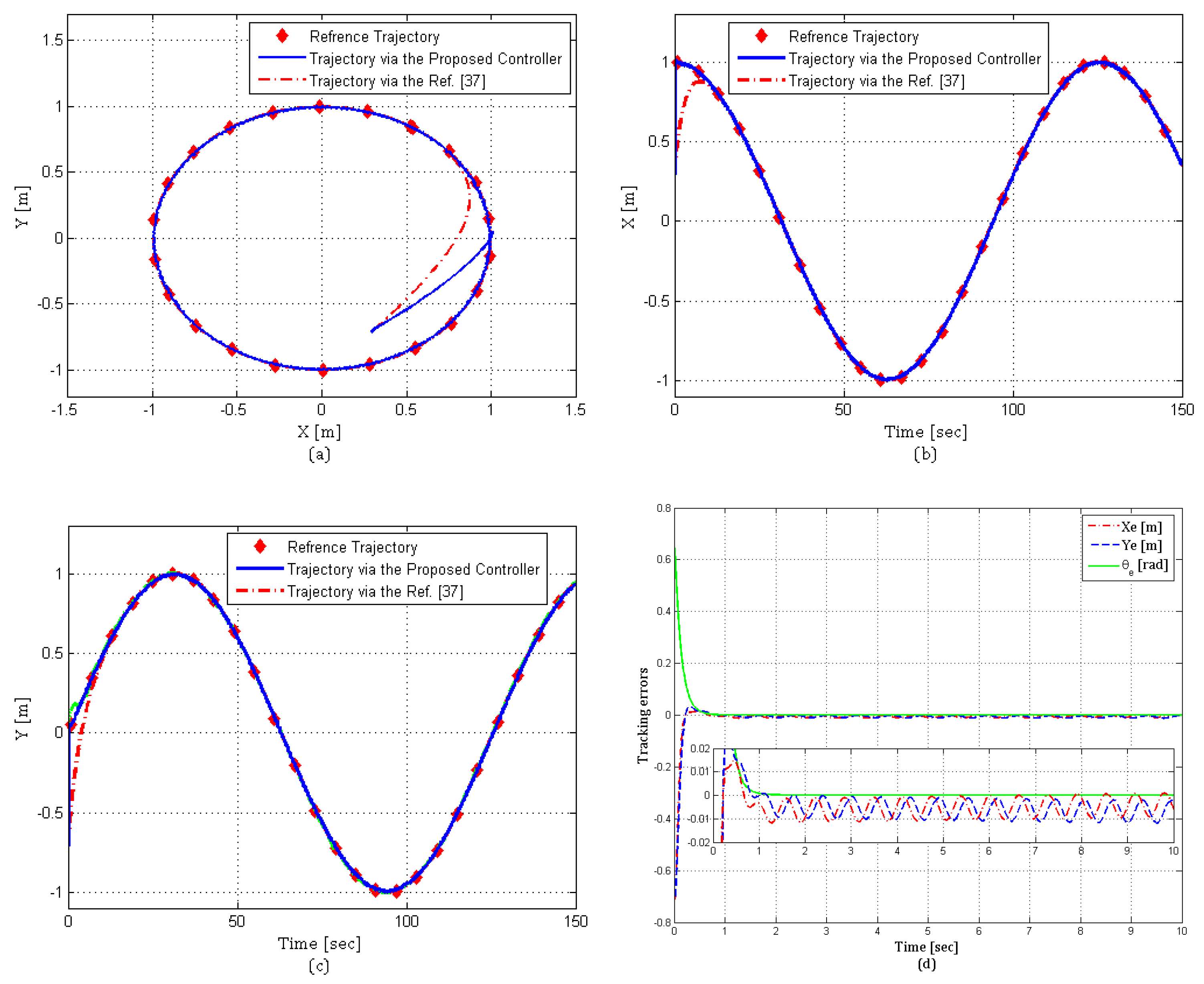
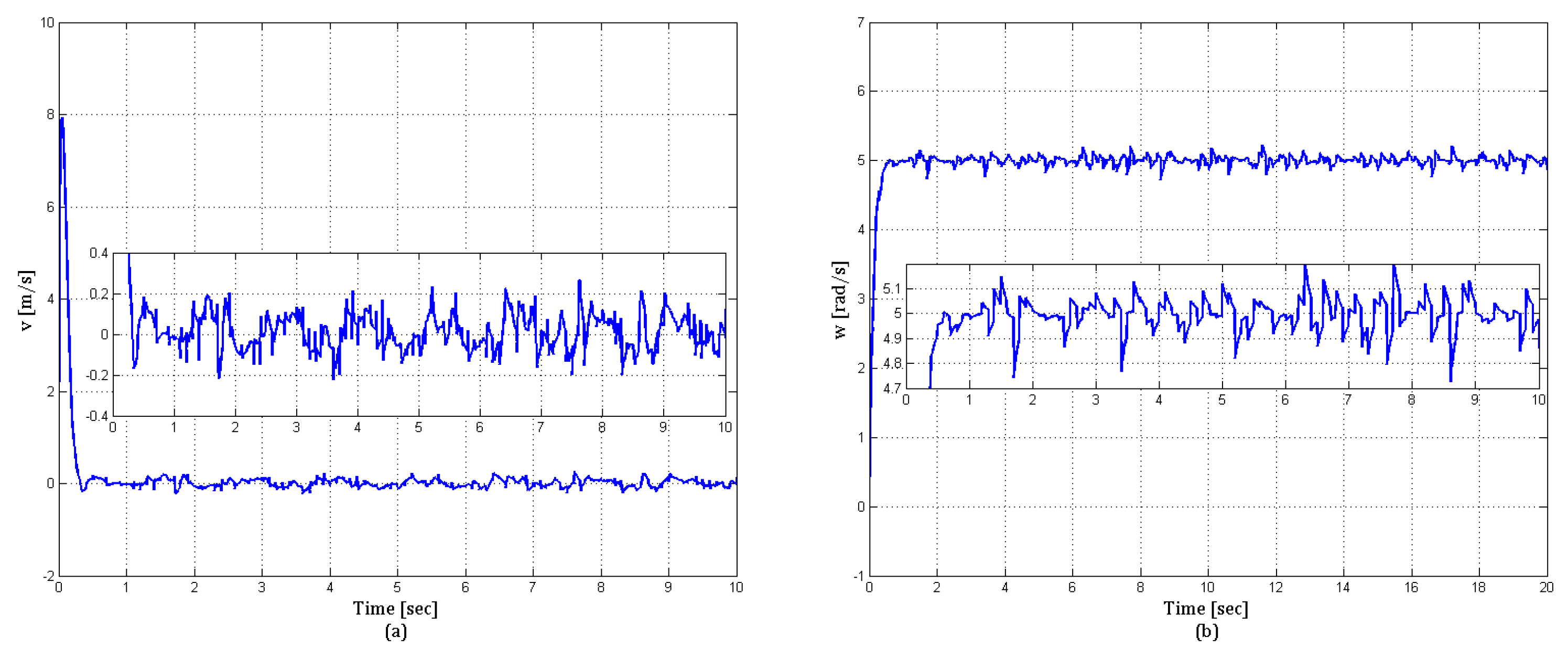
6.1. Simulation Results for Trajectory Tracking

The state-space model of WMR (Equation (13)) is simulated under the control law (Equation (23)), with the substitution of auxiliary control input u from Equations (57) and (58) calculated using the backstepping control technique. The block diagram of the backstepping controller is displayed in Figure 2. The performance of the proposed controller is compared with the previous method [37] during circular trajectory tracking. Moreover, the efficiency of the proposed controller is tested in the presence of white noise during the lemniscate curve trajectory. WMR physical parameters are selected to match with a real-world mobile robot, as summarized in

Table 1. System parameters.

Parameter	Description	Value
r	Radius of wheels	0.05 m
$2L$	Distance between two driving wheels	0.27 m
m	Mass of robot	4 kg
I	Moment of inertia of whole robot	2.5 kg·m${}^2$
d	Distance from point $p_0$ to point $p_c$	0.05 m

. During the first simulation, a circular trajectory can be defined as:

$$\begin{array}{cc}\hfill x_r\left(t\right)& =\cos \left(0.05t\right)\hfill \\ \hfill y_r\left(t\right)& =\sin \left(0.05t\right)\hfill \end{array}$$

(74)

The second simulation is performed on a lemniscate curve trajectory, which produces constantly changing both linear and angular velocities as WMR is subject to a real application problem. Lemniscate trajectory can be obtained as:

$$\begin{array}{cc}\hfill x_r\left(t\right)& =\sin \left(0.04t\right)\hfill \\ \hfill y_r\left(t\right)& =\sin \left(0.08t\right)\hfill \end{array}$$

(75)

Simulation results of circular and lemniscate curve trajectories are shown in Figure 3 and Figure 4 and Figure 5 and Figure 6, respectively. We used the same control parameters for both simulations, as shown in

Table 2. Controller parameters.

Parameter	Trajectory Tracking	Posture Stabilization
$k_1$	2.5	2.5
$k_2$	8	6
$k_3$	6.5	6
$k_4$	60	20
$k_5$	9	10
${\dot{\theta }}_r$	5 (rad/s)	0
$\left(x\right(0),y(0),\theta (0\left)\right)$	(0.3, −0.7, $37°$)	(−5, −5, $90°$), Figure 7 and Figure 8 and
		(0, −1, $180°$), Figure 9 and Figure 10

.

In particular, Figure 3a shows the trajectory tracking of WMR to a reference trajectory appropriately in the $x-y$ plane. Conversely, Figure 3b,c displays the mobile robot trajectory tracking in x and y coordinates, respectively. The obtained results show that both generalized coordinates follow the reference trajectories smoothly with a good transient response as compared with that of the previous control law in [37]. Figure 3d, displays the asymptotic convergence of error trajectories ($x_e$, $y_e$, ${\theta }_e$) to zero to ensure successful tracking of mobile robot in x, y, and $\theta$ directions. The key advantage of using normal form representation of WMR made the proposed controllers in Equations (57) and (58) simple proportional-derivative (PD) controllers because of the features of the regular backstepping technique as compared with block-backstepping controller in Equations (21) and (31) in [37]. The aforementioned controller in [37] has a complex mathematical formulation that required a large computational effort by incorporating proportional, integral, and derivative action. Figure 4a,b shows the linear and angular velocities of WMR, respectively, which are computed using the actual robot motion commands (7), i.e., wheels velocities.

The higher controller gain of $k_4$ leads to minimizing tracking error in x and y trajectories and a lower settling time (mobile robot cancels the position error quickly to track the reference trajectory). Conversely, a lower controller gain will degrade tracking performance and result in more tracking errors in x and y directions.

The performance of the proposed controller is further tested in the presence of white noise. The white noise with signal power 0.01 and 0.05 are introduced in right and left wheel velocities, respectively. It can be observed in Figure 5a–c that proposed controller successfully tracks the lemniscate curve trajectory in the $x-y$ plane. Furthermore, Figure 5d, displays the asymptotic convergence of error trajectories ($x_e$, $y_e$, and ${\theta }_e$) to zero in the presence of white noise. Figure 6a and Figure 6b show the linear and angular velocities of WMR, respectively, due to the measurement noise in wheel velocities. The RMS error of both trajectories is shown in

Table 3. Root mean square error (RMSE) of trajectory tracking.

Parameter	Circular Trajectory	Lamniscate Curve Trajectory
x (m)	0.0114	0.0123
y (m)	0.0117	0.0123
$\theta$ (rad)	0.0097	0.0109

.

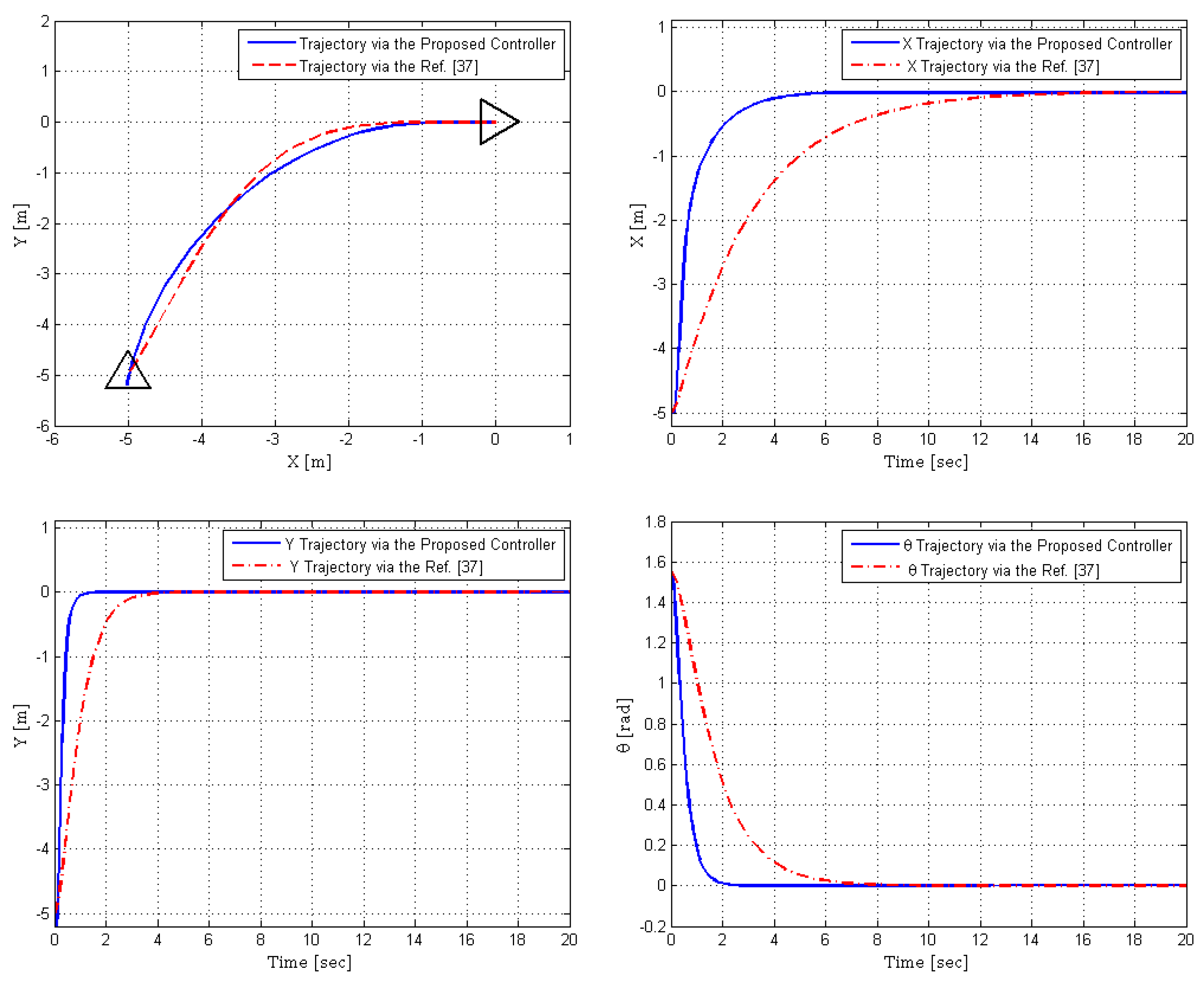
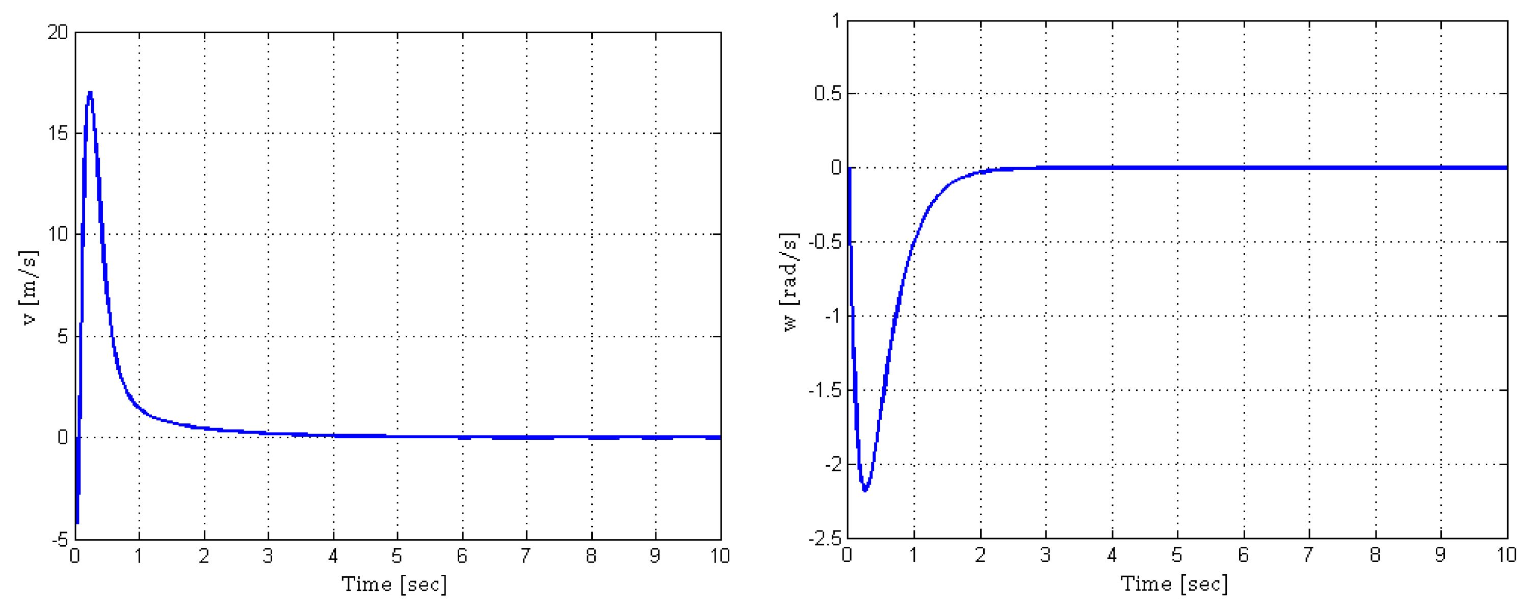
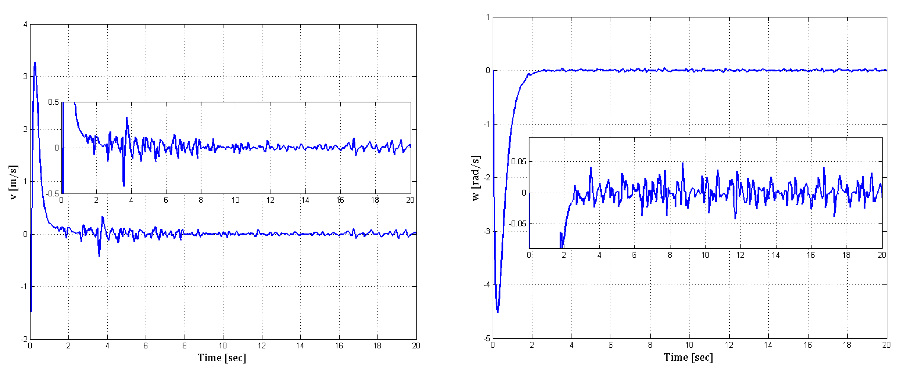
6.2. Simulation Results for Posture Stabilization

The simulation results show the posture stabilization of WMR for two scenarios: (1) forward parking and (2) parallel parking. We used the same control parameters for both scenarios, as shown in Table 2. The performance of the proposed controller is compared with the previous method in [37] during forward parking. Moreover, the efficiency of the proposed controller is tested in the presence of white noise during parallel parking. Figure 7 demonstrates the posture stabilization of the mobile robot for forward parking. The results show the posture stabilization of WMR to origin from the initial posture (−5, −5, $90°$) in the $x-y$ plane. Moreover, the state trajectories of the robot’s $(x,y)$ position and orientation angle quickly converge to zero as compared with that of the previous controller in [37]. Figure 8 shows the linear and angular velocities of WMR, which are computed using the actual robot motion commands (Equation (7)), i.e., wheels velocities.

Conversely, Figure 9 and Figure 10 show the posture stabilization of the mobile robot during parallel parking in the presence of white noise. The white noise with signal powers 0.015 and 0.001 are introduced in right and left wheel velocities, respectively. It can be observed in Figure 9 that the proposed controller successfully stabilizes the WMR to origin from initial posture (0, −1, $180°$) even in the presence of disturbance. Furthermore, Figure 9 shows the state trajectories of the robot’s $(x,y)$ position and orientation angle convergence to zero with negligible error due to external disturbance. Figure 10 shows some distortion in linear and angular velocities of WMR due to the measurement noise in wheel velocities.

7. Conclusions

This research proposes a novel generalized nontriangular normal form for a class of underactuated nonholonomic systems, i.e., WMR by a suitable change of coordinates (diffeomorphism) transformation, with structural properties that provide ease of design to the controller. Based on the generalized nontriangular normal form, a novel backstepping approach is proposed to achieve stabilization and tracking of WMR, which has not been achieved in the past. The most challenging part of this research is the asymptotic stabilization of the internal dynamics of the proposed nontriangular normal form. Due to its internal dynamics being not minimum phase and non-strict feedback form structure during both scenarios. During trajectory tracking, the effectiveness of the proposed controller is tested on different trajectories, including a circular and lemniscate curve. Conversely, for posture stabilization, both forward parking and parallel parking are examined. With the input-to-state stability of internal dynamics, the Lyapunov stability function was used to ensure the semi-global asymptotic stability of the entire closed-loop system, except around the origin of $\theta \left(0\right)\ne 0$. The silent features of the proposed controller are the fast transient response and tracking error rejection. From a practical perspective, the proposed backstepping controller would provide simple control law expression to implement in the hardware platform and robustness against the uncertainties. Indeed, one of the significant features of the proposed normal form for WMR would be the design of an output feedback controller using a high gain observer that can recover the performance of the state feedback controller for systems represented in normal form to leave out velocity sensors that can cause measurement noise. From a practical viewpoint, the controller can be further improved in order to provide an actuator-level control signal.

References

1. Bloch, A.M.; Reyhanoglu, M.; McClamroch, N.H. Control and stabilization of nonholonomic dynamic systems. IEEE Trans. Autom. Control 1992, 37, 1746–1757. [Google Scholar] [CrossRef]
2. Campion, G.; d’Andrea-Novel, B.; Bastin, G. Modelling and state feedback control of nonholonomic mechanical systems. In Proceedings of the 30th IEEE Conference on Decision and Control, Brighton, UK, 11 December 1991; pp. 1184–1189. [Google Scholar]
3. Sun, W.; Tang, S.; Gao, H.; Zhao, J. Two time-scale tracking control of nonholonomic wheeled mobile robots. IEEE Trans. Control Syst. Technol. 2016, 24, 2059–2069. [Google Scholar] [CrossRef]
4. Xiao, H.; Li, Z.; Yang, C.; Zhang, L.; Yuan, P.; Ding, L.; Wang, T. Robust stabilization of a wheeled mobile robot using model predictive control based on neurodynamics optimization. IEEE Trans. Ind. Electron. 2016, 64, 505–516. [Google Scholar] [CrossRef] [Green Version]
5. Wang, D.; Xu, G. Full-state tracking and internal dynamics of nonholonomic wheeled mobile robots. IEEE/ASME Trans. Mechatron. 2003, 8, 203–214. [Google Scholar] [CrossRef]
6. Oriolo, G.; De Luca, A.; Vendittelli, M. WMR control via dynamic feedback linearization: Design, implementation, and experimental validation. IEEE Trans. Control Syst. Technol. 2002, 10, 835–852. [Google Scholar] [CrossRef]
7. Brockett, R.W. Asymptotic stability and feedback stabilization. Differ. Geom. Control Theory 1983, 27, 181–191. [Google Scholar]
8. Sun, S.; Cui, P. Path tracking and a practical point stabilization of mobile robot. Robot. Comput. Integr. Manuf. 2004, 20, 29–34. [Google Scholar] [CrossRef]
9. Chen, H. Robust stabilization for a class of dynamic feedback uncertain nonholonomic mobile robots with input saturation. Int. J. Control Autom. Syst. 2014, 12, 1216–1224. [Google Scholar] [CrossRef]
10. Liang, Z.; Wang, C. Robust exponential stabilization of nonholonomic wheeled mobile robots with unknown visual parameters. J. Control Theory Appl. 2011, 9, 295–301. [Google Scholar] [CrossRef]
11. Coelho, P.; Nunes, U. Path-following control of mobile robots in presence of uncertainties. IEEE Trans. Robot. 2005, 21, 252–261. [Google Scholar] [CrossRef]
12. Montoya-Villegas, L.; Moreno-Valenzuela, J.; Pérez-Alcocer, R. A feedback linearization-based motion controller for a UWMR with experimental evaluations. Robotica 2019, 37, 1073–1089. [Google Scholar] [CrossRef]
13. Liang, X.; Wang, H.; Chen, W.; Guo, D.; Liu, T. Adaptive image-based trajectory tracking control of wheeled mobile robots with an uncalibrated fixed camera. IEEE Trans. Control Syst. Technol. 2015, 23, 2266–2282. [Google Scholar] [CrossRef]
14. Sarrafan, N.; Shojaei, K. High-Gain Observer-Based Neural Adaptive Feedback Linearizing Control of a Team of Wheeled Mobile Robots. Robotica 2020, 38, 69–87. [Google Scholar] [CrossRef]
15. Yamamoto, Y.; Yun, X. Coordinating locomotion and manipulation of a mobile manipulator. In Proceedings of the 31st IEEE Conference on Decision and Control, Tucson, AZ, USA, 16 December 1992; pp. 2643–2648. [Google Scholar]
16. Yun, X.; Yamamoto, Y. Stability analysis of the internal dynamics of a wheeled mobile robot. J. Robot. Syst. 1997, 14, 697–709. [Google Scholar] [CrossRef]
17. Coelho, P.; Nunes, U. Lie algebra application to mobile robot control: A tutorial. Robotica 2003, 21, 483–493. [Google Scholar] [CrossRef]
18. Al-Mutib, K.; Abdessemed, F.; Hedjar, R.; Alsulaiman, M.; Bencherif, M.; Faisal, M.; Algabri, M.; Mekhtiche, M. Mobile robot nonlinear feedback control based on Elman neural network observer. Adv. Mech. Eng. 2015, 7, 1–14. [Google Scholar] [CrossRef]
19. Eghtesad, M.; Necsulescu, D.S. Study of the internal dynamics of an autonomous mobile robot. Robot. Auton. Syst. 2006, 54, 342–349. [Google Scholar] [CrossRef]
20. Chwa, D. Tracking control of differential-drive wheeled mobile robots using a backstepping-like feedback linearization. IEEE Trans. Syst. Man Cybern.-Part A Syst. Hum. 2010, 40, 1285–1295. [Google Scholar] [CrossRef]
21. Chwa, D. Robust distance-based tracking control of wheeled mobile robots using vision sensors in the presence of kinematic disturbances. IEEE Trans. Ind. Electron. 2016, 63, 6172–6183. [Google Scholar] [CrossRef]
22. Mnif, F. Recursive backstepping stabilization of a wheeled mobile robot. Int. J. Adv. Robot. Syst. 2004, 1, 25. [Google Scholar] [CrossRef] [Green Version]
23. Andreev, A.; Peregudova, O. Lyapunov vector function method in the motion stabilisation problem for nonholonomic mobile robot. Int. J. Syst. Sci. 2017, 48, 2003–2012. [Google Scholar] [CrossRef]
24. Alshamali, S. A backstepping design approach to a class of mobile robots. In Proceedings of the 11th Asian Control Conference (ASCC), Gold Coast, QLD, Australia, 17–20 December 2017; pp. 1341–1344. [Google Scholar]
25. Wu, X.; Jin, P.; Zou, T.; Qi, Z.; Xiao, H.; Lou, P. Backstepping trajectory tracking based on fuzzy sliding mode control for differential mobile robots. J. Intell. Robot. Syst. 2019, 96, 109–121. [Google Scholar] [CrossRef]
26. Ascencio, P.; Astolfi, A.; Parisini, T. Backstepping pde design: A convex optimization approach. IEEE Trans. Autom. Control 2017, 63, 1943–1958. [Google Scholar] [CrossRef] [Green Version]
27. Asif, M.; Khan, M.J.; Memon, A.Y. Integral terminal sliding mode formation control of non-holonomic robots using leader follower approach. Robotica 2017, 35, 1473–1487. [Google Scholar] [CrossRef]
28. Memon, A.Y.; Khalil, H.K. Output regulation of nonlinear systems using conditional servocompensators. Automatica 2010, 46, 1119–1128. [Google Scholar] [CrossRef]
29. Olfati-Saber, R. Nonlinear Control of Underactuated Mechanical Systems with Application to Robotics and Aerospace Vehicles. Ph.D. Thesis, Massachusetts Institute of Technology, Cambridge, MA, USA, 2001. [Google Scholar]
30. Zhang, X.; Wang, R.; Fang, Y.; Li, B.; Ma, B. Acceleration-level pseudo-dynamic visual servoing of mobile robots with backstepping and dynamic surface control. IEEE Trans. Syst. Man Cybern. Syst. 2017, 49, 2071–2081. [Google Scholar] [CrossRef]
31. Sun, K.; Sui, S.; Tong, S. Fuzzy adaptive decentralized optimal control for strict feedback nonlinear large-scale systems. IEEE Trans. Cybern. 2017, 48, 1326–1339. [Google Scholar] [CrossRef]
32. Jiang, J.; Astolfi, A. Under-actuated back-stepping: An introduction. In Proceedings of the IEEE Conference on Decision and Control (CDC), Miami Beach, FL, USA, 17–19 December 2018; pp. 5910–5915. [Google Scholar]
33. Herzig, N.; Moreau, R.; Redarce, T.; Abry, F.; Brun, X. Nonlinear position and stiffness Backstepping controller for a two Degrees of Freedom pneumatic robot. Control Eng. Pract. 2018, 73, 26–39. [Google Scholar] [CrossRef]
34. Moghanni-Bavil-Olyaei, M.R.; Ghanbari, A.; Keighobadi, J. Trajectory Tracking Control of a Class of Underactuated Mechanical Systems with Nontriangular Normal Form Based on Block Backstepping Approach. J. Intell. Robot. Syst. 2019, 96, 209–221. [Google Scholar] [CrossRef]
35. Fu, J.; Chai, T.; Su, C.Y.; Jin, Y. Motion/force tracking control of nonholonomic mechanical systems via combining cascaded design and backstepping. Automatica 2013, 49, 3682–3686. [Google Scholar] [CrossRef]
36. Zhao, X.; Wang, X.; Zhang, S.; Zong, G. Adaptive neural backstepping control design for a class of nonsmooth nonlinear systems. IEEE Trans. Syst. Man Cybern. Syst. 2018, 49, 1820–1831. [Google Scholar] [CrossRef]
37. Rudra, S.; Barai, R.K.; Maitra, M. Design and implementation of a block-backstepping based tracking control for nonholonomic wheeled mobile robot. Int. J. Robust Nonlinear Control 2016, 26, 3018–3035. [Google Scholar] [CrossRef]
38. Fu, J.; Tian, F.; Chai, T.; Jing, Y.; Li, Z.; Su, C.Y. Motion tracking control design for a class of nonholonomic mobile robot systems. IEEE Trans. Syst. Man Cybern. Syst. 2018, 50, 2150–2156. [Google Scholar] [CrossRef]
39. Wang, Z.; Li, G.; Chen, X.; Zhang, H.; Chen, Q. Simultaneous stabilization and tracking of nonholonomic WMRs with input constraints: Controller design and experimental validation. IEEE Trans. Ind. Electron. 2018, 66, 5343–5352. [Google Scholar] [CrossRef]
40. Byrnes, C.I.; Isidori, A. A frequency domain philosophy for nonlinear systems, with applications to stabilization and to adaptive control. In Proceedings of the 23rd IEEE Conference on Decision and Control, Las Vegas, NV, USA, 12–14 December 1984; pp. 1569–1573. [Google Scholar]
41. Rubio Hervas, J. Dynamics and Control of Higher-Order Nonholonomic Systems. Ph.D. Thesis, Embry-Riddle Aeronautical University, Daytona Beach, FL, USA, 2013. [Google Scholar]
Figure 1. The wheel mobile robot.
Electronics 10 01992 g001
Figure 2. Block diagram of the backstepping controller for stabilization and tracking of WMR.
Electronics 10 01992 g002
Figure 3. Circular trajectory tracking of WMR. In (a) x-y plot. (b) Trajectory tracking in x direction. (c) Trajectory tracking in y direction. (d) Tracking errors ( x e , y e , θ e ).
Electronics 10 01992 g003
Figure 4. Circular trajectory tracking: (a) linear velocity v (m/s) and (b) angular velocity ω (rad/s).
Electronics 10 01992 g004
Figure 5. Lemniscate curve trajectory tracking of WMR with white noise. In (a) x-y plot. (b) Trajectory tracking in x direction. (c) Trajectory tracking in y direction. (d) Tracking errors ( x e , y e , θ e ).
Electronics 10 01992 g005
Figure 6. Lemniscate curve trajectory tracking with white noise: (a) linear velocity v (m/s) and (b) angular velocity ω (rad/s).
Electronics 10 01992 g006
Figure 7. Posture stabilization (forward parking with initial heading angle at 90 ° ).
Electronics 10 01992 g007
Figure 8. Posture stabilization (forward parking with initial heading angle at 90 ° ): linear velocity v (m/s) and angular velocity ω (rad/s).
Electronics 10 01992 g008
Figure 9. Posture stabilization with White Noise (parallel parking with initial heading angle at 180 ° ).
Electronics 10 01992 g009
Figure 10. Posture stabilization with White Noise (parallel parking with initial heading angle at 180 ° ): linear velocity v (m/s) and angular velocity ω (rad/s).
Electronics 10 01992 g010