Designing 1D Chaotic Maps for Fast Chaotic Image Encryption

Abstract

Chaotic maps that can provide highly secure key sequences and ease of structure implementation are predominant requirements in image encryption systems. One Dimensional (1D) chaotic maps have the advantage of a simple structure and can be easily implemented by software and hardware. However, key sequences produced by 1D chaotic maps are not adequately secure. Therefore, to improve the 1D chaotic maps sequence security, we propose two chaotic maps: 1D Improved Logistic Map (1D-ILM) and 1D Improved Quadratic Map (1D-IQM). The proposed maps have shown higher efficiency than existing maps in terms of Lyapunov exponent, complexity, wider chaotic range, and higher sensitivity. Additionally, we present an efficient and fast encryption method based on 1D-ILM and 1D-IQM to enhance image encryption system performance. This paper also introduces a key expansion method to reduce the number of chaotic map iteration needs, thereby decreasing encryption time. The security analyses and experimental results are confirmed that 2D Correlation Coefficient (CC) Information Entropy (IE), Number of Pixels Change Rate (NPCR), Unified Average Changing Intensity (UACI), Mean Absolute Error (MAE), and decryption quality are able to meet the encryption security demands (CC = −0.00139, IE = 7.9990, NPCR = 99.6114%, UACI = 33.46952% and MAE = 85.3473). Furthermore, the proposed keyspace reaches 10²⁴⁰, and the encryption time is 0.025s for an image with a size of 256 × 256. The proposed system can yield efficacious security results compared to obtained results from other encryption systems.

1. Introduction

Due to the massive multimedia technology progression, transmitting digital images through the Internet and mobile communications networks have gained increasing popularity. At the same time, digital image processing technology and the security of images transmitted through public networks have also gained much attention. Image encryption is an effective technique to prohibit unauthorised access of images from public networks. Due to the inherent characteristics of the digital images, such as the bulk data capacity, high redundancy, and robust correlation, conventional methods of the image encryption such as the International Data Encryption Algorithm, Data Encryption Standard (DES), and Advanced Encryption Standard (AES), could not meet the demands of acceptable digital image encryption [1]. To overcome this problem, the researchers suggested numerous cipher methods from several perspectives, in providing sufficient security for the multimedia information, for example, the substitution box (S-box)-based encryption [2], DNA coding-based encryption [3], wave function-based encryption [4], compressive sensing-based encryption [5], Latin square [6], and chaos [7,8,9]. Among the technologies, the Chaos method of image encryption is an excellent and effective one. This is so because chaotic maps have a significant level of sensitivity to the control parameters and initial values, and are characterised by non-convergence, chaotic, and ergodicity. For these reasons, a considerable number of algorithms of chaotic image encryption were developed by the direct utilisation of the available chaotic maps to their processes of encryption [10]. Generally, an algorithm of chaos-based image encryption includes two essential parts: a chaotic map and an image encryption system. The chaotic maps in algorithms of image encryption can be categorised into two classes: high dimensional (HD) and one dimensional (1D). HD chaotic maps have an increased image security applications [11] due to the fact that they have multiple parameters and highly complicated structures. In spite of the fact that the HD chaotic maps have highly complicated structures, their execution time is slow, and their hardware/software implementations are difficult [12]. On the other hand, 1D chaotic maps have problems with their chaotic behaviour and chaotic range. Nevertheless, due to their simple structure and ease of implementation [13], the 1D chaotic maps have been widely utilised. It has been found that the main problems of 1D chaotic maps are: (a) the chaotic range is relatively limited; (b) there is non-uniform distribution of data of the output chaotic sequences; (c) the proposed key is not sufficiently secure; (d) the attacks on random sequences are fast with a rather low computational cost. Consequently, some researchers have suggested an improved version of existing 1D chaotic maps in order to overcome 1D chaotic maps problems [14,15,16,17,18], while other researchers have suggested some novel 1D chaotic maps [19,20].

In the image encryption system that is based on chaotic maps, the encryption system includes a pair of linear (i.e., permutation) -non-linear (i.e., diffusion) conversions. Some of the encryption systems are repeating this procedure to raise the encryption strength [21,22,23,24,25]. However, in those algorithms, a large number of iterations of chaotic maps is required to produce large sequences to be utilised in permutation and diffusion steps. Consequently, a high number of iterations can lead to high encryption time. For chaotic cryptosystems, the chaotic maps have a significant impact in developing excellent chaotic image encryption systems. Nonetheless, we must pay more attention to the steps of confusion and diffusion to make the encryption system valid against differential encryption attacks.

This research addresses the defects of the Logistic map and Quadratic map. Hence, an improved version of these maps (1D-ILM and 1D-IQM) is proposed in order to overcome the defects. In addition, an encryption system for images is proposed in this paper, which utilises the 1D-ILM and 1D-IQM to satisfy the security and protection needs of a digital image before being transmitted in a public network. The proposed image scheme is designed to meet the requirements of security to defeat several encryption-attack types. The implementation of encryption and decryption’s scheme is simple and fast.

The key contributions of this paper are summarised as follows:

• A new method to improve 1D chaotic maps is designed to overcome the problems of 1D chaotic maps.
• A new key generation scheme is designed to update the initial keys according to information of plaintext image, and a new key expansion method is used to reduce the number of chaotic map iterations.
• In the diffusion phase, not only is the value of pixel modified but it is also shifted based on the location value of pixels and chaotic sequences.
• The proposed system not only provides a high degree of security but also ensures a low encryption time and a simple computational process.

This article is organised as follows. Section 2 presents related work. Section 3 reviews the performance of existing chaotic maps. Section 4 introduces the new chaotic map and demonstrate its accuracy. Section 5 includes the proposed encryption method. Section 6 provides experimental results and analysis, and Section 7 concludes the paper.

2. Related Work

Over the previous decade, many researchers have attention to present developed and improved image encryption algorithms.

In [26], Herbadji et al. presented an enhanced Quadratic map with enhanced chaotic range to be utilised in colour image cryptosystem. The encryption system includes two rounds of the permutation-diffusion process. The diffusion step is applied in which the three image components are simultaneously encrypted. The security analysis demonstrates the efficiency of the proposed cryptosystem in colour images, although it is not able to encrypt grey-scale images.

In [27], Pak et al. proposed an improved 1D chaotic map made with output sequences of two of the same classical 1-D chaotic maps. The proposed map applications are successfully employed in colour and grey images cryptosystem consisting of permutation, diffusion, and linear transformation steps. In the case of colour image encryption, the chaotic sequence generated in this algorithm needs a high number of iterations to fit all image pixels, thus, taking up a high execution time.

In [28], Ge et al. proposed a symmetric encryption algorithm based on a new chaotic map. The proposed map is used in an encryption system, consisting of two phases: bit-pair level process and pixel-level diffusion. The proposed chaotic map has multiple parameters which can provide good security. On the other hand, the proposed map is relatively complex and needs a high execution time. This is because the map consists of complex trigonometric functions and many conditions determined in each iteration.

In [29], Huang et al. introduced a tweak-cube cryptosystem based on a new 1D chaotic map and a 4D hyper-chaotic map. The suggested map is associated with a 4D map to generate key streams utilised in diffusion and scramble steps. The proposed 1D map behaviour becomes chaotic only in specific regions. Tiny perturbation to the chaotic map parameter can make the parameter enter a nonchaotic part, thereby making the encryption key not secure.

In [30], Pak and Huang suggested enhanced 1D chaotic maps. The enhanced chaotic maps have been generated by combining two classical 1D chaotic maps. Based on those enhanced maps, a cryptosystem with steps of linear-nonlinear-linear conversion is introduced to improve the security of image encryption. The enhanced chaotic maps show superior chaotic properties compared with the classical maps. The proposed encryption system shows adequate security results, but the number of chaotic map iteration needs is considerably high, making the encryption system relatively slow.

In [31], Yavuz et al. suggested encryption based on two chaotic functions, where the encryption system consists of confusion and diffusion principles. In order to provide high resistance against differential attacks, additional operations of circular rotation and XOR are applied on the encrypted image. The algorithm has a good security analysis, but the process of encryption/decryption is complicated and hard to implement, thus making the encryption system not applicable. Furthermore, ideal encryption needs more than three encryption rounds.

Wang et al. [32] have suggested a fast algorithm for encrypting images based on logistic maps that simultaneously performed the operations of diffusion and permutation. Therefore, the number of iterations is decreased to reduce the computational time. The suggested algorithm is capable of resisting the chosen plain text attacks. However, its keyspace is not adequately large in order to endure the statistical attacks, and the effect of the scrambling step is not optimal.

In [33], Liu et al. introduced a fast scheme that simultaneously performs the diffusion and permutation. This cryptosystem has good capability for withstanding the chosen plaintext attacks and low execution time. Nonetheless, it was unsuccessful in resisting the data loss and noise attacks.

In [34], a grey image encryption scheme is presented using a 6D chaotic map combined with Fibonacci Q-matrix. The 6D chaotic map is used to scramble the positions of image pixels, where the Fibonacci Q-matrix is used to diffuse the pixels. The 6D chaotic map provides sufficient keyspace that is able to challenge the differential attacks.

In [35], Liu et al. have introduced a fast method for image encryption in which the processes of permutation and diffusion are simultaneously performed. The row and the column techniques are performed in this method to reduce the processing time. This proposed method showed efficient security and good speed performance.

In [36], Ding and Ding combine 2D chaotic map and 4D Chaotic map with 2D Discrete Wavelet Transform (DWT) to produce a new image encryption system. The authors prove that the encrypted image has high keyspace and security. However, the utilisation of HD chaotic map with DWT increases the complexity in hardware/software implementation.

In [37], a fast encryption method based on chaos, DNA encryption technique, and parallel compressive sensing is introduced. The parallel compressive sensing technique is employed to speed up the encryption system by minimizing the size of the image.

3. D Chaotic Map

The chaotic map has been produced with a non-linear dynamic system. A specific range of its control parameters can have a strong sensitivity to its initial values. In this section, we will discuss the Logistic map and Quadratic map in brief.

3.1. Logistic Map

The Logistic map is an efficient and simple 1D chaotic map that has a complicated, chaotic behaviour, and it can be represented by the equation below:

$$x_{n+1}=LM\left({m,x}_n\right) {=m\times x}_n{\times (1-x}_n)$$

(1)

m represents a control parameter with ranges of (0, 4], and $x_n$ represents the chaotic output sequence with range [0, 1]. The Logistic map can be chaotic only when $m$ is in the range of [3.57, 4.0], and if the control parameter m is higher than the range, the logistic map cannot be having chaotic behaviours [30]. The bifurcation diagram of the map is capable of the objective reflection of the state and the region of a map’s chaotic behaviour. The Logistic map’s bifurcation diagram is depicted in Figure 1a. The 1D chaotic map includes a single largest Lyapunov exponent (LE), used to measure whether a map is chaotic. If the value of the LE is bigger than 0, the map can be considered chaotic and the other way around. With the increase of the value of the LE, the complexity of the map is increased (i.e., it becomes less predictable). The LE for the 1D maps is defined in Equation (2), and Figure 2a shows the LE diagram of the Logistic chaotic map.

$$\mathrm{LE}=\underset{n\to \infty }{\lim }\frac{1}{n}{\displaystyle \sum }_{i=0}^{n-1}\ln \left|f^{\prime }\left(x_i\right)\right|,$$

(2)

where $f^{\prime }\left(x\right)$ indicates the derivative function of function f (x), while f (x) indicates a 1D chaotic map. n is the number of chaotic map iterations.

For the Logistic map output sequence, there are two main drawbacks that are illustrated as follows:

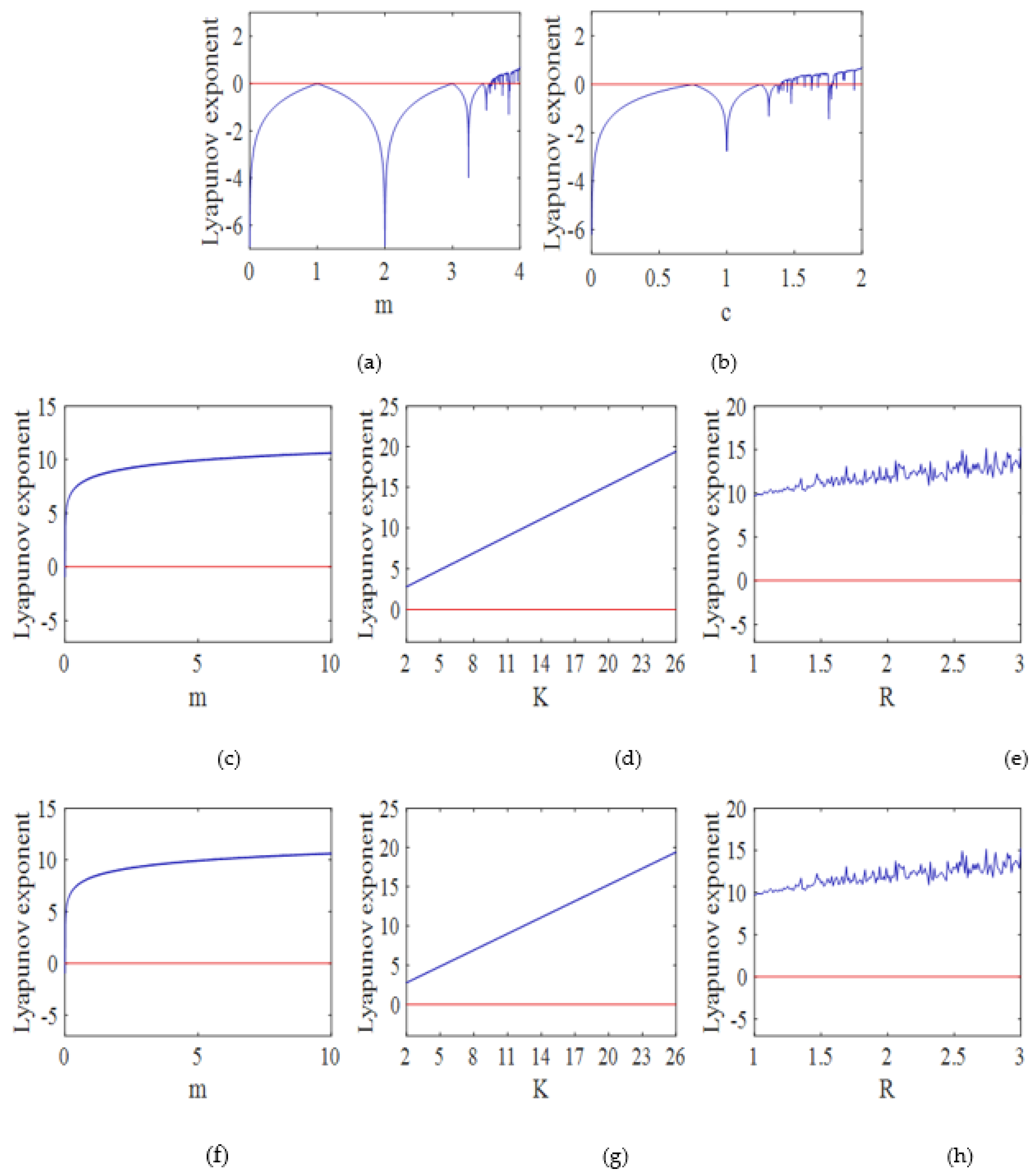
• The sequence of the Logistic map can be chaotic only when parameter $m$ in the range of [3.57, 4.0], which has been verified by the negative values in the curve of LE diagram that is shown in Figure 2a.
• Even in the range of $m$ ∈ [3.57, 4.0], there are values that result in no chaotic behaviours in the Logistic map. This has been verified by the blank area in the diagram of the bifurcation that is shown in Figure 1a.

The encryption system must have a close relation to the encryption key, so it is essential to use a sufficient and secure encryption key. The encryption key produced by the Logistic map is relatively small. Only parameter $m$ and initial state $x_0$ are utilised as initial keys for the Logistic chaotic sequence causing the Logistic map applications to be narrowed down. As a result, it is essential to select a high complexity chaotic map to design the encryption algorithm.

3.2. Quadratic Map

The conventional Quadratic map can be defined as the famed chaotic map that has high complexity dynamic behaviour. This map is commonly utilised in the applications of cryptography. The Quadratic map equation can be seen below:

$$v_{n+1}=QM\left({c,v}_n\right) =c- {{(v}_n)}^2$$

(3)

Here, $c$ represents the controlling parameter that has the range [0, 2], $v_n$ ∈ [−2, 2] represents the produced chaotic sequence. In the case of parameter $c$ ∈ [1.4, 2.0], the Quadratic map has a chaotic behaviour [26]. Even when $c$ ∈ [1.4, 2.0], there are some values that make the quadratic map has no chaotic sequence. Similar to the logistic map, the Quadratic map has the same problems. The bifurcation and LE diagrams are illustrated in Figure 1b and Figure 2b.

4. New Chaotic Maps

This section includes the proposed new chaotic map. To verify its precision, the abovementioned 1D chaotic maps have been utilised.

4.1. System Designing

The new chaotic map has been characterised using the equation below,

$$x_{n+1}{=F(m,x}_n{,K,R)=(\left(\right(F}_{chaos}{(m,x}_n{\left)\right)\times 2}^K{)/sin(x}_n{)}^R)\mathrm{mod}1$$

(4)

where ${F(m,x}_n,K,R)$ represents a new chaotic map. $F_{chaos}\left(m,x_n\right)$ is an existing 1D chaotic map (one of the abovementioned). m, K and R represent control parameters with a wide range. The mod represents module operation, which is utilised to make sure that the produced chaotic sequence is confined in the [0, 1] range. ${F(m,x}_n,K,R)$ has a chaotic characteristic in an expanded range that is larger than the existing range of 1D chaotic maps. In the case of the parameters K and R in the range of [2, 26] and [1, 3], respectively, the new suggested chaotic map has a high complex chaotic behaviour. The m, K and R range has been experimentally confirmed by bifurcation and LE in the following subsection. The new suggested chaotic system structure is simple, and it can be easily implemented by hardware as well as software.

4.2. System Verified

To verify the suggested chaotic system’s efficiency, the abovementioned 1D chaotic maps have been utilised as follows.

4.2.1. 1D-ILM

In this subsection, the improved version of the Logistic map (1D-ILM) is presented using Equation (4). The presented chaotic map can overcome the problems mentioned in Section 3, making it more appropriate for designing cryptosystems. The improved Logistic map (1D-ILM) can be represented in Equation (5),

$$x_{n+1} {=F}_L\left({m,x}_n\right) =\left(\right((m {\times x}_n {\times (1-x}_n{\left)\right)\times 2}^K)/sin{\left(x_n\right)}^R)\mathrm{mod}1$$

(5)

where the parameter m ∈ (0, $10$]. Parameters K and R in the range of [2, 26] and [1, 3], $x_n$ represents the initial value of the sequence, where $x_n\ne 0$. $n$ represents the number of iterations. The bifurcation diagram of 1D-ILM is shown in Figure 1c–e. The 1D-ILM sequence can exhibit uniform distributions in the range within [0, 1]. Additionally, according to the LE curve that is shown in Figure 2c–e, the results of LE are positive at all values of m ∈ (0.1, 10] K ∈ [2, 26] and R ∈ [1, 3]. As a result, the chaotic range and the chaotic characteristics of 1D-ILM are efficient, and 1D-ILM is appropriate to be employed in the encryption algorithm.

4.2.2. 1D-IQM

For the purpose of generating a chaotic sequence that has an adequate chaotic efficiency, the Quadratic map is modified with the use of Equation (4). The map is referred to as the 1D-Improved Quadratic Map (1D-IQM). The modified equation is as follows:

$$v_{n+1} {=F}_Q\left({c,v}_n\right) {=\left(\right((c-(v}_n{)}^2{)\times 2}^K{)/sin(v}_n{)}^R)\mathrm{mod}1$$

(6)

c, K, and R represent the control parameters, and $v_n$ represents the initial map’s value within (0, 1]. K ∈ [2, 26] and R ∈ [1, 3]. According to the observations that have been provided in Figure 2f–h, the proposed 1D-IQM exhibits positive LE values (its chaotic conduct) when c ∈ [0, 10], K ∈ [2, 26] and R ∈ [1, 3]. The chaotic sequences that are generated using 1D-IQM are uniformly distributed in the range of [0, 1], as illustrated in Figure 1f–h.

4.2.3. Application to Other Maps

Numerous 1D chaotic maps are able to be improved with the use of the suggested system designing (Equation (4)).

4.3. Performance Evaluation

The new chaotic maps will be evaluated using phase diagram (Attractor), approximate entropy, sensitivity, and uniformity. For simplicity, the value of K and R of 1D-ILM and 1D-IQM are set to 12 and 1 respectively.

4.3.1. Phase Diagram of Chaotic Map

Chaotic systems have outputs of higher randomness in the case where its chaos phase diagram is capable of occupying a bigger phase space. As observed in Figure 3c,d, the output sequence of 1D-ILM and 1D-IQM maps fill a bigger region than the regular Logistic and Quadratic maps sequences in the 2D phase diagram. This means that the 1D-ILM and 1D-IQM sequences have better randomness and ergodicity and are more convenient to be used in image encryption systems. From Figure 4, the Logistic and Quadratic maps have a closed trajectory and significant structure in 3D phase space. On the contrary, the 1D-ILM and 1D-IQM show no closed trajectory, indicating better randomness.

4.3.2. Approximate Entropy (Complexity)

The fundamental concept of the Approximate Entropy (ApEn) algorithm is using a non-negative value to quantify the time series irregularity, unpredictability, and complexity. Moreover, the larger the computed value of the ApEn, the more complex is the sequence produced by a chaotic map [38]. The specific details of the ApEn calculation can be found in [39]. Besides the proposed chaotic maps, three chaotic maps (1DSP [20], LFHCM [29], EQM3 [26]) are compared with the proposed maps. The ApEn diagrams are shown in Figure 5. From Figure 5, the suggested chaotic maps have better ApEn, proving that they can produce sequences with higher unpredictability and complexity.

4.3.3. Map Sensitivity

The chaotic maps used in the cryptosystem should be sensitive to the initial value and the control parameters [28]. In order to test the sensitivity level of the proposed chaotic maps, the following procedures will be followed:

• The chaotic map is iterated 100 times to form the first chaotic sequence.
• The chaotic map is re-iterated after tiny changes to one of its parameters to form the second sequence.
• The trajectories of the two generated sequences are compared.

Figure 6 shows the map sensitivity results. The difference between the two trajectories of 1D-ILM and 1D-IQM can be visually distinguishable after nearly five iterations, as shown in Figure 6c,d. In regard to the Logistic map and Quadratic map in Figure 6a,b, the difference is distinguishable after nearly 50 iterations. From this result, the 1D-ILM and 1D-IQM have better sensitivity to their parameters.

4.3.4. Sequence Uniformity

The uniform distribution of the sequences is an indication of the fact that the sequence is robustly random and it has preferable secure performance [40]. On the other hand, in the case of the non-uniform distribution of the sequences, the sequences are not secure, and the statistical attacks have sufficient attack effects. The uneven distribution is an indication that the output sequence randomness is insufficient. The sequence uniformity analysis for chaotic maps can be shown in Figure 7, where the distribution of the Logistic map and Quadratic map is uneven. Consequently, their randomness is relatively poor, and their safety performance, weak. On the other hand, the proposed maps 1D-ILM and 1D-IQM are uniformly distributed, thereby proving significant randomness and preferable security performance.

5. Image Encryption System Based on 1D-ILM and 1D-IQM

The architecture for the proposed encryption system is shown in Figure 8, which consists of two main phases: permutation phase and diffusion phase.

5.1. Key Generation Scheme

Key generation scheme steps of the encryption scheme with the use of Message-Digest Algorithm (MD5) are introduced in this subsection, where MD5 is a cryptographic hash function that plays an essential role in image encryption. MD5 can generate a 128-bit hash value [41]. As MD5 is irreversible, it can resist different types of attacks, such as known-plaintext attacks.

In the proposed encryption scheme, the initial values, and parameters of 1D-ILM and 1D-IQM are the secret keys. To make the secret key mainly dependent on image pixels and image size, the following steps will be followed:

Step 1: Suppose the plaintext image P$\left(M,N\right)$, where M indicates the number of the rows while N indicates the number of columns, we calculate ${sum}_P$, where ${sum}_P$ represents the sum of all pixel values of P.

Step 2: We calculate two vectors: ${sum}_R$ with the size of M and ${sum}_C$ with the size of $N$, where ${sum}_R$ is the sum of each row of P and ${sum}_C$ is the sum of each column of $P$. Then, the MD5 hash of $su{m}_R$ and $su{m}_C$ is calculated to generate $R_{hash}$ and $C_{hash}$ with 128-bit hash value. Divide $R_{hash}$ and $C_{hash}$ into 8-bit (2-byte) blocks in decimal format as expressed in the following equations.

$$\left\{\begin{array}{c}{R}_{hash}=\mathrm{MD}5\left({sum}_R\right)\hfill \\ R_{hash}= \left\{r_1{,r}_2{,\dots r}_{16}\right\}\hfill \end{array}\right.$$

(7)

$$\left\{\begin{array}{c}{C}_{hash}=\mathrm{MD}5\left({sum}_C\right)\hfill \\ C_{hash}= \left\{c_1{,c}_2{,\dots c}_{16}\right\}\hfill \end{array}\right.$$

(8)

Since the MD5 is very sensitive to any minor changes, one-bit change in $P$ can lead to a significant difference in the hash values ($R_{hash}{,C}_{hash}$). After that, we generate four values based on hash values ($R_{hash}{,C}_{hash}$) using XOR operation $\left(\oplus \right)$ as in the following equations,

$$\left\{\begin{array}{c}{R}_{Key1}{=r}_1\oplus r_2\oplus \dots \oplus r_8\hfill \\ R_{Key2} {=r}_9\oplus r_{10}\oplus \dots \oplus r_{16}\hfill \end{array}\right.$$

(9)

$$\left\{\begin{array}{c}{C}_{Key1}= c_1\oplus c_2\oplus \dots \oplus c_8\hfill \\ C_{Key2}= c_9\oplus c_{10}\oplus \dots \oplus c_{16}\hfill \end{array}\right.$$

(10)

Step 3: Suppose the initial keys ${\ddot{x}}_1$, ${\ddot{x}}_2$, ${\ddot{v}}_1$, ${\ddot{v}}_2$, ${\ddot{m}}_1$, ${\ddot{m}}_2$, ${\ddot{c}}_1$ and ${\ddot{c}}_2$ are randomly selected. Then, the initial keys are updated according to the plain image pixel value as follows:

$$\left\{\begin{array}{c}{x}_1= ({\ddot{x}}_1{\mathrm{mod}R}_{Key1})/256\\ x_2= ({\ddot{x}}_2{\mathrm{mod}R}_{Key2})/256\\ v_1= ({\ddot{v}}_1{\mathrm{mod}C}_{Key1})/256\\ v_2= ({\ddot{v}}_2{\mathrm{mod}C}_{Key2})/256\end{array}\right.$$

(11)

$$\left\{\begin{array}{c}{m}_1= \left(\left({sum}_{p}mod{\ddot{m}}_1\right)\times \left({sum}_P/M\right)\right)\mathrm{mod}9+1\\ m_2= \left(\left({sum}_{p}mod{\ddot{m}}_2\right)\times \left({sum}_P/M\right)\right)\mathrm{mod}9+1\\ c_1= \left(\left({sum}_{p}mod{\ddot{c}}_1\right)\times \left({sum}_P/N\right)\right)\mathrm{mod}9+1\\ c_2= \left(\left({sum}_{p}mod{\ddot{c}}_2\right)\times \left({sum}_P/N\right)\right)\mathrm{mod}9+1\end{array}\right.$$

(12)

Step 4: 1D-ILM is firstly iterated ($M$ + 100 times) using $x_1$ and $m_1$ and secondly iterated using $x_2$ and $m_2$ to form two chaotic sequences $X1$ and $X2,$ respectively. After that, the 1D-IQM is firstly iterated ($N$ + 100 times) using $v_1$ and $c_1$ and secondly iterated using $v_2$ and $c_2$ to form two chaotic sequences $Y1$ and $Y2,$ respectively. The First 100 elements of sequences $X1$, $X2$, $Y1$ and $Y2$ are discarded in order to improve the sensitivity of initial values and parameters of the map (to avert transient effect).

Step 5: After the chaotic sequences $X1(M,1)$, $X2(M,1)$, $Y1(1,N)$ and $Y2(1,N)$ are generated by 1D-ILM and 1D-IQM, we propose a key expansion method to reduce the number of iteration as well as the encryption time especially in large-sized images. By using a multiply operation between $X1(M,1)$ and $Y1(1,N)$ and between $X2(M,1)$ and $Y2(1,N)$, we obtain two chaotic matrices $S_1$ $(M,N)$ and $S_2(M,N)$ respectively. Then, they are manipulated together to form a chaotic matrix $S$($M,N$) as expressed in Equation (13), which has the same size as the input image.

$$S= (\left(S_1{+S}_2\right)\times 1000)\mathrm{mod} E_{key}$$

(13)

where $E_{key}$ is a secret key. For each value of $E_{key}$, we have a unique chaotic sequence of $S$. Numerical example of the key expansion method is depicted in Figure 9. The chaotic sequences of the proposed encryption system are directly related to the plaintext image. In the case of minor changes in pixel value or size of plaintext image that occurs, the value of $su{m}_P$, $su{m}_R$ and $su{m}_C$ will change. Consequentially, the initial value ($x_1$, $x_2$, $v_1$, $v_2$), parameters ($m_1$, $m_2$, $c_1$, $c_2$) and chaotic sequences ($X1$, $X2$, $Y1$, $Y2$) will significantly change. This is because the proposed chaotic maps and the proposed key generation scheme are extremely sensitive to any minor changes.

5.2. Permutation Phase

There is a natural high correlation between the neighbouring pixels in the relevant plaintext image. A good encryption method has to be capable of decreasing that correlation and obscuring the positions of the pixels and making the original image to meaningless chaotic image so that the pixel positions are arranged in a random and unorderly manner.

In the proposed permutation phase, a new permutation scheme using chaotic matrix $S$ to alter the location of all pixels of plaintext image chaotically is proposed. The permutation phase is illustrated in the following steps:

Step 1: Sort the $S$ in ascending order by performing Equation (14)

$$\left[S_{\mathit{sorted}}{,S}_{\mathit{index}}\right] =\mathit{sort}\left(S\right),$$

(14)

where $S_{\mathit{sorted}}$ represents the sorted sequence of $S$, and $S_{\mathit{index}}$ represents the index value of $S_{\mathit{sorted}}$.

Step 2: The pixels positions of P are re-arranged according to the index matrix ($S_{\mathit{index}}$). After all the pixels of P are moved to their new positions, the permuted image $P_P$ is generated.

5.3. Diffusion Phase

Chosen plaintext attacks have been designed for breaking the encryption system by examining how a minor change in plaintext images can affect the system’s encryption results. An efficient diffusion phase is able to make an image encryption system withstand those types of attacks. In the proposed diffusion phase, the column diffusion and row diffusion techniques are used in which the pixels of an image are diffused by columns and then by rows. The diffusion steps are illustrated in the following steps:

Step 1: Convert the chaotic sequences $X1$, $X2$, $Y1$ and $Y2$ into integer sequences by using the following equations,

$$\begin{gathered} I_{X1}{= \lceil X1\times R}_{Key1}\times L1\rceil \mathrm{mod}M, \\ {I}_{Y1}{ = \lceil Y1\times C}_{Key1}\times L2\rceil \mathrm{mod}N, \\ {I}_{X2}{ = \lceil X2\times R}_{Key2}\times L3\rceil \mathrm{mod}M, \\ {I}_{Y2}{ = \lceil Y2\times C}_{Key2}\times L4\rceil \mathrm{mod}N, \end{gathered}$$

(15)

where $\lceil .\rceil$ represents floor function, $L1$, $L2$, $L3,$ and $L4$ are integer values $\in \left(1000,4000\right)$.

Step 2: Chaotic matrix $S$ is converted into integer form to produce diffusion matrix $D$ as in Equation (16).

$$D {= \lfloor S\times (R}_{Key1}{+C}_{Key1})\times L5\rfloor \mathrm{mod}256,$$

(16)

where $\lfloor .\rfloor$ represents ceil function, $L5$ $\in \left(1000,4000\right)$.

Step 3: Apply Column Diffusion. The image pixels can be chaotically encrypted by using the value of two previous encrypted pixels to encrypt the current one. For column diffusion, Equation (17) is applied.

$$\left\{\begin{array}{c}{E}^C\left(.,1\right) = \left[\left(P_P\left(.,1\right) + \left(C_{Key1}\times I_{Y1}\left(1\right)\right)\right) \mathrm{mod}256\right] \oplus D\left(.,I_{Y1}\left(1\right)\right)\hfill \\ E^C\left(.,2\right) = \left[\left(P_P\left(.,2\right) + \left(E^C\left(.,1\right) + C_{Key1}\right) \times I_{Y1}\left(2\right)\right) \mathrm{mod}256\right] \oplus D\left(.,I_{Y1}\left(2\right)\right)\hfill \\ E^C\left(.,j\right) = \left[\left(P_P\left(.,j\right) + \left(E^C\left(.,j-1\right) \times I_{Y1}\left(j - 1\right)\right) + \left(E^C\left(.,j - 2\right) \times I_{Y1}\left(j-2\right)\right) + \left(C_{Key2}\times I_{Y1}\left(j\right)\right)\right) \mathrm{mod}256\right] \oplus D\left(.,I_{Y1}\left(j\right)\right)\hfill \end{array}\right.$$

(17)

where j from 3 to N. And then chaotic column shift is applied to shuffle the columns as in the following expression,

$$\left\{\begin{array}{c}{E}_s^C\left(i,j\right){ =E}^C\left({i,j+I}_{Y2}\left(i\right)\right)\hspace{1em}\hspace{1em}\hspace{1em}\hspace{1em}\hspace{1em}\hspace{1em}\hspace{1em}\hspace{1em} j + I_{Y2}\left(i\right)\le N\\ E_s^C\left(i,j\right){ =E}^C\left({i,j+I}_{Y2}\left(i\right) - N\right)\hspace{1em}\hspace{1em}\hspace{1em}\hspace{1em}\hspace{1em}\hspace{1em}j + I_{Y2}\left(i\right)>N\end{array}\right.$$

(18)

where i from 1 to M, j from 1 to N.

Step 4: Apply row Diffusion. Encrypt the image rows according to Equation (19).

$$\left\{\begin{array}{c}{E}^R\left(1,.\right) = \left[\left(E_s^C\left(1,.\right) + \left(R_{Key1}\times I_{X1}\left(1\right)\right)\right) \mathrm{mod}256\right] \oplus D\left(I_{X1}\left(1\right),.\right)\hfill \\ E^R\left(2,.\right) = \left[\left(E_s^C\left(2,.\right) + \left(E^R\left(1,.\right) + R_{Key1}\right) \times I_{X1}\left(2\right)\right) \mathrm{mod}256\right] \oplus D\left(I_{X1}\left(2\right),.\right)\hfill \\ E^R\left(i,.\right) = \left[\left(E_s^C\left(i,.\right) + \left(E^R\left(i-1,.\right) \times I_{X1}\left(i - 1\right)\right) + \left(E^R\left(i - 2,.\right) \times I_{X1}\left(i-2\right)\right) + \left(R_{Key2}\times I_{X1}\left(i\right)\right)\right) \mathrm{mod}256\right] \oplus D\left(I_{X1}\left(i\right),.\right)\hfill \end{array}\right.$$

(19)

where i from 3 to M. After that, shift the rows of image as in Equation (20),

$$\left\{\begin{array}{c}{E}_s^R\left(i,j\right){ =E}^R\left({i+I}_{X2}\left(j\right),j\right){\hspace{1em}\hspace{1em}\hspace{1em}\hspace{1em}\hspace{1em}\hspace{1em}\hspace{1em}\hspace{1em} i+I}_{X2}\left(j\right)\le M\\ E_s^R\left(i,j\right){ =E}^R\left({i+I}_{X2}\left(j\right) - M,j\right){\hspace{1em}\hspace{1em}\hspace{1em}\hspace{1em}\hspace{1em}\hspace{1em}i+I}_{X2}\left(j\right)>M\end{array}\right.$$

(20)

where i from 1 to M, j from 1 to N.

The chaotic row and column shift is used to increase the security and is also used to increase the encryption system sensitivity. After the diffusion phase is completed, the encrypted image is generated. It is evident that the decryption process is similar to the encryption process but in a reverse way. The encrypted images can be shown in Figure 10.

5.4. Extended to Colour Images

In the case of a colour image, it is encrypted by splitting the image components, Red (R), Green (G) and Blue (B). We then treat each component as a grey image. In consequence, the encryption of each component is exactly similar to the proposed encryption steps. Following that, we combine the result of the encryption process of each component to obtain the encrypted image. The encrypted colour images are shown in Figure 11.

6. Performance Analysis

The test images consist of standard Lena image of size 512 × 512, and 9 grey images have been chosen from the USC-SIPI Image Database. The secret keys in the encryption algorithm are selected as follows:

${\ddot{x}}_1$ = 1000.567, ${\ddot{x}}_2=$ 1344.455, ${\ddot{v}}_1$ = 2000.345, ${\ddot{v}}_2$ = 1235.345, ${\ddot{m}}_1$ = 4, ${\ddot{m}}_2$ = 3, ${\ddot{c}}_1$ = 2, ${\ddot{c}}_2$ = 3, $L1=$ 2600, $L2=3500$, $L3=3000$ and $L4=$ $L5=1000.$ K and R for 1D-ILM and IQM are set to 12 and 1, respectively. MATLAB R2015a with Intel Core i7-4600 CPU @2.7GHz and 8GB RAM on Windows 10 operating system.

6.1. Statistical Analysis

In this work, three indicators used to evaluate the capability of the proposed image encryption system towards resisting statistical attacks are histogram analysis, correlation analysis, and entropy.

6.1.1. Histogram Analysis

The histogram exhibits the pixel intensity value distribution for a grey image. Figure 12a illustrates plain image histograms. Figure 12b shows that the encrypted image results of even distribution at a [0, 255] interval. It entirely differs from the histogram of the plain image. Based on Figure 12c, the decrypted image results completely preserve the plain image information. In consequence, it becomes hard for the attackers to predict plain images using statistical analyses.

To further prove the histogram uniformity of the proposed encryption system, the Chi-square test $\left(x^2\right)$ is utilised, where the Chi-square test ($x^2$) indicates a statistical measure of the distribution of pixels. The formula of the Chi-square test ($x^2$) can be justified below [42].

$$x^2={{\displaystyle \sum }}_i^{256}\frac{{{(P}_i-256)}^2}{256},$$

(21)

where $i$ represents the levels number of the grey-scale and $P_i$ ∈ (0–255) represents the observed frequency occurrences of the grey levels. The value of the Chi-square test ($x^2$) for the encrypted images should be close or below the theoretical value 293.24783 [35]. The results of Chi-square test ($x^2$) are tabulated in

Table 1. Chi-square test.

Image	Plain Image	Encrypted Image
Lena	114,486.457	233.779
Boat	383,969.687	239.060
Couple	298,865.244	261.164
Tank	957,952.570	259.609
Elaine	140,667.152	237.857
Stream and bridge	1,185,618.347	245.048
Man	709,340.680	293.547
Airport	1,974,776.136	278.427
Chemical plant	50,326.4453	246.375
Clock	282,061.562	255.359
Average	609,806.400	255.022

, where the Chi-square test ($x^2$) of encrypted images are close to the theoretical one.

6.1.2. Adjacent Pixels Correlation

The adjacent pixel correlation (${\mathrm{C}}_{\mathrm{xy}}$) can be defined as one of the common ways for the evaluation of the image encryption algorithm’s performance, and an efficient cryptosystem must eliminate such intrinsic relation for the purpose of improving the resistance against the statistical analyses [43]. Equation (22) is used to calculate the correlation of adjacent pixels (${\mathrm{C}}_{\mathrm{xy}}$).

$$\begin{gathered} E\left(x\right) =\frac{1}{N}{{\displaystyle \sum }}_{i=1}^N{x}_i \\ D\left(x\right) =\frac{1}{N}{{\displaystyle \sum }}_{i=1}^N{\left(x_i-E\left(x\right)\right)}^2 \\ \mathrm{cov}\left(x,y\right) =\frac{1}{N}{{\displaystyle \sum }}_{i=1}^N\left(x_i-E\left(x\right)\right)\left(y_i-E\left(y\right)\right) \\ {\mathrm{C}}_{\mathrm{xy}}=\mathrm{cov}\left(x,y\right) / \sqrt{D\left(x\right)}\sqrt{D\left(y\right)}, \end{gathered}$$

(22)

where x and y represent the grey-scale values of two pixels that are adjacent in location. N represents the entire number of the x and y obtained from an image.

Table 2. Correlation analysis.

Image	Plaintext Image			Encrypted Image			2D-CC
	Horizontal	Vertical	Diagonal	Horizontal	Vertical	Diagonal
Lena	0.97380	0.98564	0.96039	−0.000805	−0.000776	0.003297	0.001463
Boat	0.93812	0.97131	0.92216	0.001051	0.000723	0.000096	0.002264
Couple	0.93707	0.89264	0.85572	−0.00168	0.001695	−0.000275	0.001045
Tank	0.96566	0.93040	0.91676	0.000832	0.000673	−0.003580	−0.003580
Elaine	0.97565	0.97302	0.96925	0.000989	−0.001817	−0.001210	−0.000595
Stream and bridge	0.94041	0.92751	0.89749	0.000407	−0.003383	0.001103	−0.004226
Man	0.97745	0.98127	0.96715	0.001012	−0.000191	0.001548	−0.000125
Airport	0.90993	0.90337	0.85905	−0.001955	−0.000400	−0.000430	0.000143
Chemical plant	0.94662	0.89841	0.85291	0.0019064	−0.000793	−0.001858	−0.005777
Clock	0.95649	0.97408	0.93893	0.0080607	−0.001130	0.000842	−0.004517
Average	0.95212	0.943765	0.913981	0.000982	−0.00054	−0.000046	−0.00139

lists the Correlation (${\mathrm{C}}_{\mathrm{xy}}$) values for various plain images as well as their equivalent encrypted images.

The correlation values of the ideal ciphering system have to approach the 0 value. Table 2 shows that the correlation values of encrypted images are noticeably decreased (the values are very close to the 0 value). Additionally,

Table 3. Correlation comparison.

Algorithm	Proposed	Ref. [28]	Ref. [44]	Ref. [45]	Ref. [46]
Horizontal	−0.000805	0.0054	0.0019	−0.0056	−0.0022
Vertical	−0.000776	0.0064	−0.0024	0.0006	0.0015
Diagonal	0.003297	0.0046	0.0011	0.0018	0.0025

lists the comparison with different algorithms. In addition, the adjacent pixel distributions in three various directions are illustrated in Figure 13. As can be seen, from Figure 13a,c,e, the plaintext image has a robust correlation between the neighbouring pixels in the three directions; vertical, horizontal and diagonal. From Figure 13b,d,f, the cipher image points are full of space and are chaotically distributed. Evidently, the pixel value correlations between two neighbouring encrypted image points are considerably decreased.

6.1.3. Correlations between Original and Encrypted Image

The 2D Correlation Coefficient (CC) between different plain/cipher-image pairs have been analysed through the calculation of the 2D Correlations Coefficient (CC) between the plaintext image and its corresponding encrypted image [47]. The CC can be computed as in the following equation:

$$\mathrm{CC}=\frac{{{\displaystyle \sum }}_{i=1}^M{{\displaystyle \sum }}_{j=1}^N\left(X_{ij}-\overline{X}\right)\left(Y_{ij}-\overline{Y}\right)}{\sqrt{\left({{\displaystyle \sum }}_{i=1}^M{{\displaystyle \sum }}_{j=1}^N{\left(X_{ij}-\overline{X}\right)}^2\right)\left({{\displaystyle \sum }}_{i=1}^M{{\displaystyle \sum }}_{j=1}^N{\left(Y_{ij}-\overline{Y}\right)}^2\right)}}$$

(23)

$X_{ij}$ denotes plaintext image and $Y_{ij}$ denotes cipher-image. $\overline{X}$ and $\overline{Y}$ represent the average values of $X_{ij}$ and $Y_{ij}$ elements, respectively. M and N indicate the number of rows and columns of the cipher and plaintext images, respectively. The values of the CC of various plain images have been listed in Table 2. The values in Table 2 are very close to optimal value. i.e., 0.

6.1.4. Information Entropy (IE)

Here, IE is utilised for the evaluation of image randomness, and an information source entropy is:

$$\mathrm{IE}\left(n\right) ={{\displaystyle \sum }}_{i=0}^{N}P\left(n_i\right){\log }_2\frac{1}{P \left(n_i\right)}$$

(24)

$n_i$ denotes a source of the image, N represents a total number of the symbols and $P\left(n_i\right)$ denotes the symbol $n_i$ probability [48]. For the grey level images, the maximal IE equals 8. Results for various images are given in

Table 4. Information entropy (IE).

Image	IE
Lena	7.9994
Boat	7.9993
Couple	7.9993
Tank	7.9993
Elaine	7.9993
Stream and bridge	7.9993
Man	7.9998
Airport	7.9998
Chemical plant	7.9973
Clock	7.9972
Average	7.9990

. In addition, the entropy comparison of the encrypted Lena image is listed in

Table 5. Information entropy (IE) comparison.

Method	Proposed	Ref. [28]	Ref. [44]	Ref. [45]	Ref. [46]
IE	7.9994	7.9992	7.9993	7.9971	7.9991

. IE of the proposed algorithm remains tightly close to 8 in Table 4 and Table 5. Consequently, it is nearly impossible to obtain visual information from encrypted images.

6.2. Key Analysis

6.2.1. Key Space

A secure encryption system must have a massive keyspace that can resist attacks adequately. The keyspace size is obligated to be bigger than 2¹⁰⁰ to provide a high-security level [49]. For proposed image encryption, the parameters and initial values of chaotic maps are secret keys. The 1D-ILM has one initial value and three control parameters when R and K are considered, and 1D-IQM also has one initial value and three control parameters when R and K are considered. In the proposed scheme, each map is used twice to generate the key sequence. As a consequence, we have twelve control parameters and four initial values. In the case of precision of the initial values and parameter, it is set to 10⁻¹⁵, the keyspace equals 10^15×16 = 10²⁴⁰ ≈ 2⁷⁹⁷, which is bigger than 2¹⁰⁰. As a result, the suggested method has quite a sufficient keyspace to resist various brute-force attack types.

Table 6. Keyspace comparison.

Algorithm	Keyspace
Proposed	10240 ≈ 2797
Ref. [28]	10210 ≈ 2697
Ref. [44]	2564
Ref. [45]	2124
Ref. [46]	2199

lists the keyspace comparison between different algorithms.

6.2.2. Key Sensitivity

An efficient method of encryption must have efficient sensitivity to the secret keys. In our method, sensitivity is split into the two points below:

• Changing the key’s value throughout the encryption process causes a significant alteration to the encrypted image. The $m_1$ is tested in original secret keys. The results of the test following the slight change of $m_1$ by 10⁻¹⁵ are observed in Figure 14. The remaining secret keys are the same as above. Based on the results, the encrypted image undergoes a dramatic change in the case where the individual key has been changed 10⁻¹⁵. From such results, the proposed method has an efficient sensitivity of the encryption key.
• The slight change of the key value throughout the decryption process will have a considerable difference in the decrypted image. The test results in the case where the decryption key differs from the key of the encryption by 10⁻¹⁵ may be observed in Figure 15. Here, a considerable difference is seen between correctly and incorrectly decrypted images in the case where the decryption key differs from the key of encryption by 10⁻¹⁵. The accurately decrypted image in Figure 15d restores the original image successfully, while the inaccurately decrypted image in Figure 15c does not recognise any information compared to the original image. From this result, the proposed scheme has sufficient key sensitivity.

6.3. Analysis of the Permutation Performance

According to the permutation performance evaluation method [44], a white image with a small black square in the middle is permuted using the suggested permutation phase. The permutation phase aims to prevent the attackers from recognition of image information. If the permuted image has entirely failed in recognising the original image, it is an indication that the permutation phase is efficient. The permutation result is illustrated in Figure 16, where the black block pixels are dispersed over the whole image.

6.4. Diffusion Performance Analysis

The Differential attack, plaintext attack analysis and avalanche criterion analysis are widely utilised for the assessment of the diffusion efficiency.

6.4.1. Differential Attack Analysis

The Differential attack is considered to be a kind of plaintext attack [44]. The attackers usually make small changes to plain images and utilise the suggested encryption algorithm to encrypt the plain image of prior and post changes. By comparing those two encrypted images, they discover the correlations between the plaintext and cipher images. This type of attack is referred to as the differential attack. For the purpose of resisting the differential attacks, a small plaintext image change must result in a massive alteration in the corresponding encrypted image [50,51]. The number of Pixels Change Rate (NPCR), Unified Average Changing Intensity (UACI), and Mean Absolute Error (MAE) are three common measures that are often utilised. The NPCR and UACI can be measured according to the following equation [52].

$$\begin{gathered} D_{E_1{,E}_2}\left(i,j\right) = \left\{\begin{array}{c}{1,\hspace{1em}\hspace{1em}\hspace{1em}\hspace{1em}E}_1\left(i,j\right){ =E}_2\left(i,j\right)\\ {0,\hspace{1em}\hspace{1em}\hspace{1em}\hspace{1em}E}_1\left(i,j\right)\ne E_2\left(i,j\right)\end{array}\right. \\ \mathrm{NPCR}={{\displaystyle \sum }}_{i,j}\frac{D_{E_1{,E}_2}\left(i,j\right)}{M\times N}\times 100\% \end{gathered}$$

(25)

$$\mathrm{UACI}= \frac{1}{M\times N}{\displaystyle \sum }_{i,j}\frac{\left|E_1\left(i,j\right) - E_2\left(i,j\right)\right|}{255}\times 100\%$$

(26)

where $E_1$ and $E_2$ are equally sized images, which represent the cipher image prior and post-modification. $E_1$ represents the original ciphered image, while $E_2$ represents ciphered image after one pixel in the plaintext image is changed. The expected NPCR and UACI values for the random grey images should be within 99.6094% and 33.4635%, respectively [53]. The encrypted image results are given in

Table 7. Differential attacks.

Image	NPCR	UACI	MAE
Lena	99.6114%	33.5499%	85.5523
Boat	99.6151%	33.5107%	85.4523
Couple	99.5934%	33.4131%	85.2035
Tank	99.6063%	33.5461%	85.5426
Elaine	99.6155%	33.4066%	85.1868
Stream and bridge	99.6170%	33.4287%	85.2432
Man	99.6111%	33.4590%	85.3205
Airport	99.6066%	33.4751%	85.3615
Chemical plant	99.6124%	33.4435%	85.2808
Clock	99.6155%	33.4625%	85.3295
Average	99.6114%	33.46952%	85.3473

, and the comparison of the encrypted Lena image is listed in

Table 8. Differential attacks of Lena image.

Algorithm	Proposed	Ref. [28]	Ref. [44]	Ref. [46]
NPCR	99.61%	99.62%	99.61%	99.62%
UACI	33.54%	33.51%	33.46%	33.51%

. The NPCR and UACI of the encrypted image in Table 7 are close to the expected value (NPCR = 99.6094% and UACI = 33.4635). Therefore, the proposed encryption method has a high capability to resist differential attacks.

The Mean Absolute Error (MAE) test is another examination used to prove the validation of the encryption system in terms of differential attack [52]. MAE can be described as in the following equation.

$$\mathrm{MAE}=\frac{1}{M\times N}{\displaystyle \sum }_{i,j}\left|E_1\left(i,j\right) - E_2\left(i,j\right)\right|$$

(27)

In order to reach better encryption security, large value of $\mathrm{MAE}$ is needed. Table 7 shows the values of MAE.

6.4.2. Plaintext Attacks Analysis

The conventional cryptanalysis attacks include known-plaintext attacks, ciphertext-only attacks, chosen-ciphertext attacks, and chosen-plaintext attacks. In those four attacks, the chosen-plaintext attacks can be considered the most powerful type of attacks [54]. For this reason, it is presumed that when an encryption system is capable of resisting chosen plaintext attacks, it is capable of withstanding the other three as well [55]. Attackers usually use white or black image to recover the original images. For this reason, they are used to determine the resistance of the algorithm to the chosen plaintext attacks. The results are shown in Figure 17 and

Table 9. Chosen-plaintext attack results.

Image	Correlation			Information Entropy (IE)	Differential Attack
	Horizontal	Vertical	Diagonal		NPCR	UACI	MAE
White	0.003161	−0.000333	−0.002679	7.9992	99.6136	33.4224	85.2272
Black	0.001546	0.001025	−0.000541	7.9994	99.6143	33.4613	85.3262

. The encrypted white and black images are not comprehensible, and their histograms are uniform, as can be seen in Figure 17. From Table 9, it can be seen that the correlation in different directions is considerably decreased, and the two image entropies are close to the ideal value. Moreover, their NPCR and UACI are close to optimal values. As all tests are close to the optimum value, the chosen-plaintext attacks are efficiently resisted in the suggested algorithm of diffusion.

6.4.3. Avalanche Criterion (AC)

Evidently, changing a single bit in a plaintext image must theoretically result in a 50% difference in the bits of the cipher image [56]. The plain image will be encrypted in order to form cipher image $E_1$, and after that, a single bit of the original image is changed and the image is encrypted for forming $E_2$. Avalanche Criterion (AC) is applied between $E_1$ and $E_2$ based on Equation (28). The results are depicted in Figure 18. As shown in Figure 18, Avalanche Criterion (AC) results of the suggested model are quite close to the theoretical value.

$$\mathrm{AC}=\frac{\mathrm{Number}\mathrm{of}\mathrm{changed}\mathrm{bit}\mathrm{between} E_{1 }\mathrm{and} E_2}{\mathrm{Total}\mathrm{number}\mathrm{of}\mathrm{bit}}\times 100\%$$

(28)

6.5. Noise and Data Loss Attacks Analysis

In this subsection, the noise attacks and the data loss attacks of the proposed encryption algorithm are analysed, which is highly important in encrypted image transmission.

6.5.1. Noise Attack Analysis

For the purpose of testing the robustness of the suggested approach against the noise attacks, the following process has been performed. The original image $O_I$ has been encrypted with the use of the suggested algorithm of encryption. After that, a different density noise has been added to the encrypted image. Then, the noisy encrypted image is decrypted to form $D_I$. Results of the encrypted image with 1%, 5%, and 10% of noise density are shown in Figure 19. The Mean Square Error (MSE) is widely used to measure the average difference between $O_I$ and $D_I$. The MSE is calculated using Equation (29).

$$\mathrm{MSE}=\frac{1}{M\times N}{\displaystyle \sum }_{i=1}^M{\displaystyle \sum }_{j=1}^N{\left(O_I\left(i,j\right) - D_I\left(i,j\right)\right)}^2$$

(29)

M and N denote the entire number of rows and columns, while Peak Signal-to-Noise Ratio (PSNR) is a quantitative evaluation of similarity between $O_I$ and $D_I$. PSNR is calculated as follows:

$${\mathrm{PSNR}=10\log }_{10} \frac{I_{max}^2}{\mathrm{MSE}}$$

(30)

where $I_{max}^2$ is the maximum value of pixels of MSE. Both Figure 19 and

Table 10. Noise attack and data loss attack results.

Attack	Noise Attack			Data Lose Attack
	1% Noise	5% Noise	10% Noise	1/16 Crop	1/4 Crop	1/2 Crop
MSE	10.5007	43.0918	72.1406	17.2808	52.2921	59.7997
PSNR (dB)	19.8831	13.7393	11.4837	17.6868	12.8504	12.2726

confirmed that the encrypted images can be retrieved properly.

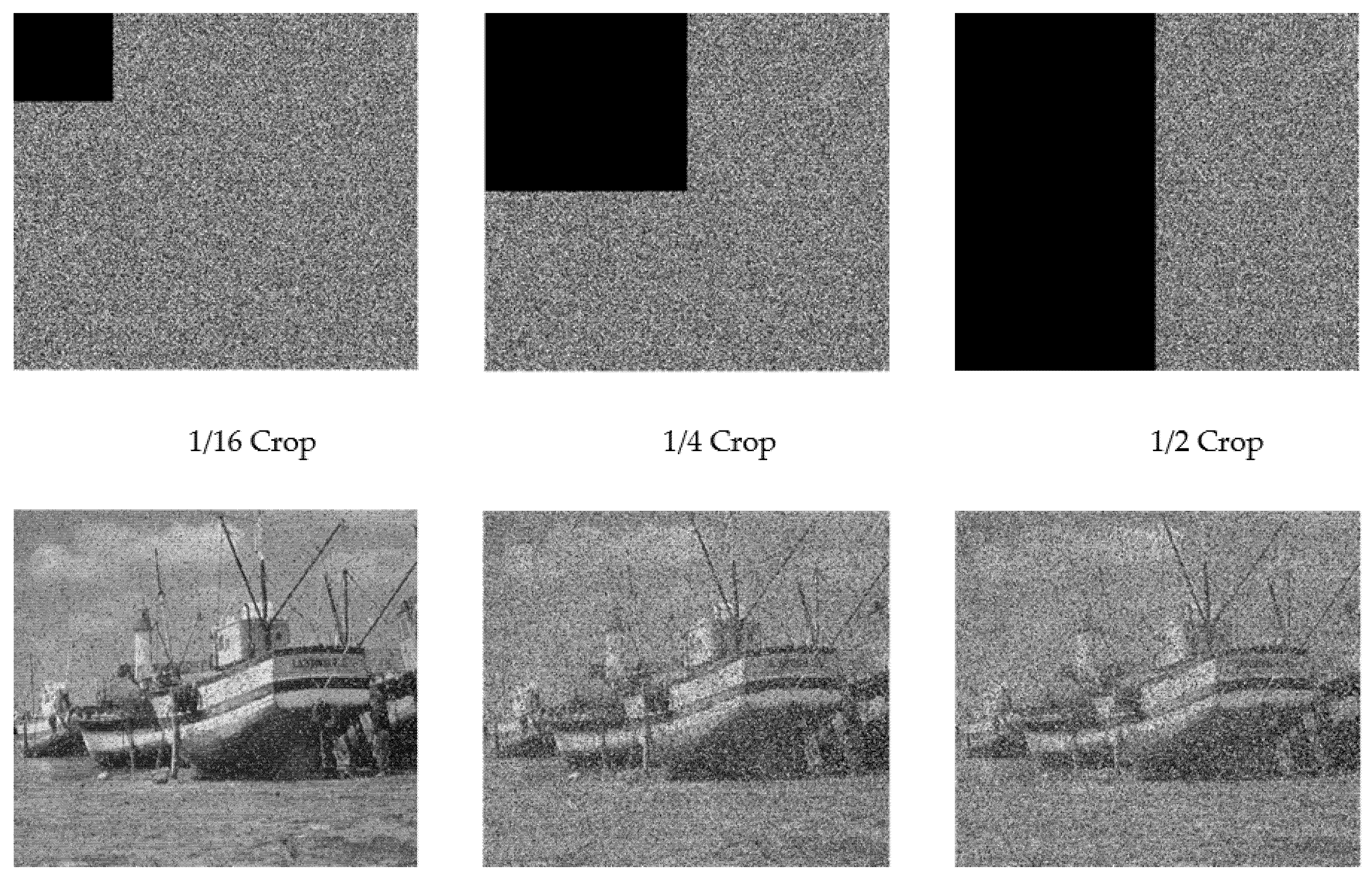
6.5.2. Data Loss Attack Analysis

Data in a different size in the encrypted image have been eliminated (Cropped) by substituting them with zeros. Following that, we try to recover the plaintext image from the encrypted image with data loss. Results of encrypted images with 1/16 data crop, 1/4 data crop and 1/2 data crop are illustrated in Figure 20. Those recovered images are also evaluated by calculating the respective MSE and PSNR. The larger calculated value of PSNR means better resistance to attacks. The result of MSE and PSNR are listed in Table 10. As can be seen from Figure 20 and Table 10, the suggested algorithm can resist various attacks (i.e., data loss attacks) in the spatial domain.

6.6. The Quality of Decryption

Decryption quality was assessed through the calculation of the 2D Correlation Coefficient (CC). For adequate decryption, CC has to be near or equal to 1. For the suggested decryption, the CC of every decrypted image equals 1, and it is proven that each decryption process is highly accurate. In other words, the decrypted image is identical to its corresponding plaintext image. Therefore, good quality has been shown in the suggested decryption.

6.7. Execution Time

Encryption speed is a necessary condition for evaluating the efficiency of cryptosystems. The experimental environment was the MATLAB R2015a with Intel Core i7-4600 CPU @2.7 GHz and 8 GB RAM on Windows 10 operating system. Taking the 256 × 256 image as an example, the results are shown in

Table 11. Encryption speed.

Algorithm	Encryption Time (s)	Processor Speed	Ram	Platform
Proposed	0.0256	2.70 GHz	8 GB	MATLAB R2015a
Ref. [28]	0.2219	2.60 GHz	8 GB	MATLAB R2013a
Ref. [44]	1.1708	3.90 GHz	4 GB	MATLAB R2014a
Ref. [45]	0.3820	3.30 GHz	4 GB	MATLAB R2016b

. In our algorithm, the result proves that the proposed encryption system has low encryption time as compared with the referenced systems.

7. Conclusions

Firstly, this paper improved two chaotic maps: 1D-ILM and 1D-ILM based on Logistic and Quadratic maps. Their performance evaluation showed that the improved maps have a large Lyapunov exponent, high complexity, wider chaotic range, and high sensitivity. Thus, they proposed efficient chaotic performance to be used in an image encryption system. Secondly, an image encryption system based on proposed maps is designed with a high-security level. The proposed scheme is very sensitive to the secret keys in which any changes can produce a completely different encrypted image. The NPCR and UACI values are close to the expected values, and the black and white image test has proven the capability of resisting the chosen-plaintext attacks. A high level of randomness of the encrypted image is proven by entropy measure and is very close to the ideal entropy value, i.e., eight. The histogram distribution is uniform for the encrypted image, and the correlation coefficient is considerably decreased between the adjacent pixels.

Additionally, the proposed scheme can effectively withstand noise and data loss attacks. Lastly, encryption schemes with a sufficient keyspace can be characterised by a long execution time. Nonetheless, the suggested system has sufficient keyspace in comparison with referenced schemes along with a shorter encryption time. This is because the proposed key expansion method can reduce the number of chaotic map iteration needs for the encryption/decryption process and thereby the execution time of the encryption system is enhanced. The proposed encryption system has a large keyspace that reaches 10²⁴⁰, and the encryption time for an image of the size of 256 × 256 is 0.025 s. In consequence, it can be efficiently utilised to transmit digital images in public networks. In future work, we will try to study three main points: (1) the effect of altering the chaotic maps on the encryption system efficiency; (2) the effect of simultaneously performing permutation and diffusion operations on processing time; (3) the effect of combining other encryption technique such as DNA technique and S-box technique with the proposed technique on encryption system robustness and security.

References

1. Zhu, H.; Zhao, C.; Zhang, X. A novel image encryption–compression scheme using hyper-chaos and Chinese remainder theorem. Signal Process. Image Commun. 2013, 28, 670–680. [Google Scholar] [CrossRef]
2. Belazi, A.; Khan, M.; El-Latif, A.A.; Belghith, S. Efficient cryptosystem approaches: S-boxes and permutation–substitution-based encryption. Nonlinear Dyn. 2017, 87, 337–361. [Google Scholar] [CrossRef]
3. Zhang, Y.; Xiao, D.; Wen, W.; Wong, K.-W. On the security of symmetric ciphers based on DNA coding. Inf. Sci. 2014, 289, 254–261. [Google Scholar] [CrossRef]
4. Huang, X.; Ye, G. An image encryption algorithm based on irregular wave representation. Multimed. Tools Appl. 2017, 77, 2611–2628. [Google Scholar] [CrossRef]
5. Li, Y.; Song, B.; Cao, R.; Zhang, Y.; Qin, H. Image Encryption Based on Compressive Sensing and Scrambled Index for Secure Multimedia Transmission. ACM Trans. Multimed. Comput. Commun. Appl. 2016, 12, 1–22. [Google Scholar] [CrossRef]
6. Panduranga, H.; Kumar, S.N. Kiran Image encryption based on permutation-substitution using chaotic map and Latin Square Image Cipher. Eur. Phys. J. Spéc. Top. 2014, 223, 1663–1677. [Google Scholar] [CrossRef]
7. Bao, L.; Zhou, Y.; Chen, C.L.P.; Liu, H. A new chaotic system for image encryption. In Proceedings of the 2012 International Conference on System Science and Engineering (ICSSE), Dalian, China, 30 June–2 July 2012; pp. 69–73. [Google Scholar]
8. Kumar, R.R.; Kumar, M.B. A new chaotic image encryption using parametric switching-based permutation and diffusion. ICTACT J. Image Video Process. 2014, 4, 795–804. [Google Scholar]
9. Liu, L.; Miao, S. An image encryption algorithm based on Baker map with varying parameter. Multimed. Tools Appl. 2017, 76, 16511–16527. [Google Scholar] [CrossRef]
10. Sathishkumar, G.A.; Sriraam, D.N. Image encryption based on diffusion and multiple chaotic maps. arXiv 2011, arXiv:1103.3792. [Google Scholar] [CrossRef]
11. Zhou, Y.; Bao, L.; Chen, C.L.P. A new 1D chaotic system for image encryption. Signal Process. 2014, 97, 172–182. [Google Scholar] [CrossRef]
12. Ye, G. Image scrambling encryption algorithm of pixel bit based on chaos map. Pattern Recognit. Lett. 2010, 31, 347–354. [Google Scholar] [CrossRef]
13. Zhang, W.; Zhu, Z.; Yu, H. A symmetric image encryption algorithm based on a coupled logistic–bernoulli map and cel-lular automata diffusion strategy. Entropy 2019, 21, 504. [Google Scholar] [CrossRef] [Green Version]
14. Hua, Z.; Zhou, Y.; Pun, C.M.; Chen, C.L.P. 2D Sine Logistic modulation map for image encryption. Inf. Sci. 2015, 297, 80–94. [Google Scholar] [CrossRef]
15. Lv-Chen, C.; Yu-Ling, L.; Sen-Hui, Q.; Jun-Xiu, L. A perturbation method to the tent map based on Lyapunov exponent and its application. Chin. Phys. B 2015, 24, 100501. [Google Scholar]
16. Herbadji, D.; Derouiche, N.; Belmeguenai, A.; Herbadji, A.; Boumerdassi, S. A Tweakable Image Encryption Algorithm Using an Improved Logistic Chaotic Map. Trait. Signal 2019, 36, 407–417. [Google Scholar] [CrossRef]
17. Song, C.-Y.; Qiao, Y.-L.; Zhang, X.-Z. An image encryption scheme based on new spatiotemporal chaos. Optik 2013, 124, 3329–3334. [Google Scholar] [CrossRef]
18. Huang, X.; Liu, L.; Li, X.; Yu, M.; Wu, Z. A New Two-Dimensional Mutual Coupled Logistic Map and Its Application for Pseudorandom Number Generator. Math. Probl. Eng. 2019, 2019, 1–10. [Google Scholar] [CrossRef] [Green Version]
19. Zhang, T.; Li, S.; Ge, R.; Yuan, M.; Ma, Y. A Novel 1D Hybrid Chaotic Map-Based Image Compression and Encryption Using Compressed Sensing and Fibonacci-Lucas Transform. Math. Probl. Eng. 2016, 2016, 1–15. [Google Scholar] [CrossRef] [Green Version]
20. Mansouri, A.; Wang, X. A novel one-dimensional sine powered chaotic map and its application in a new image encryp-tion scheme. Inf. Sci. 2020, 520, 46–62. [Google Scholar] [CrossRef]
21. Niyat, A.Y.; Moattar, M.H.; Torshiz, M.N. Color image encryption based on hybrid hyper-chaotic system and cellular automata. Opt. Lasers Eng. 2017, 90, 225–237. [Google Scholar] [CrossRef]
22. Hua, Z.; Jin, F.; Xu, B.; Huang, H. 2D Logistic-Sine-coupling map for image encryption. Signal Process. 2018, 149, 148–161. [Google Scholar] [CrossRef]
23. Shahna, K.U.; Mohamed, A. A novel image encryption scheme using both pixel level and bit level permutation with chaotic map. Appl. Soft Comput. 2020, 90, 106162. [Google Scholar]
24. Masood, F.; Driss, M.; Boulila, W.; Ahmad, J.; Rehman, S.U.; Jan, S.U.; Qayyum, A.; Buchanan, W.J. A Lightweight Chaos-Based Medical Image Encryption Scheme Using Random Shuffling and XOR Operations. Wirel. Pers. Commun. 2021, 1–28. [Google Scholar] [CrossRef]
25. Qayyum, A.; Ahmad, J.; Boulila, W.; Rubaiee, S.; Masood, F.; Khan, F.; Buchanan, W.J. Chaos-Based Confusion and Diffusion of Image Pixels Using Dynamic Substitution. IEEE Access 2020, 8, 140876–140895. [Google Scholar] [CrossRef]
26. Herbadji, D.; Belmeguenai, A.; Derouiche, N.; Liu, H. Colour image encryption scheme based on enhanced quadratic cha-otic map. IET Image Process. 2019, 14, 40–52. [Google Scholar] [CrossRef]
27. Pak, C.; An, K.; Jang, P.; Kim, J.; Kim, S. A novel bit-level color image encryption using improved 1D chaotic map. Multimedia Tools Appl. 2018, 78, 12027–12042. [Google Scholar] [CrossRef]
28. Ge, R.; Yang, G.; Wu, J.; Chen, Y.; Coatrieux, G.; Luo, L. A Novel Chaos-Based Symmetric Image Encryption Using Bit-Pair Level Process. IEEE Access 2019, 7, 99470–99480. [Google Scholar] [CrossRef]
29. Huang, L.-L.; Wang, S.-M.; Xiang, J.-H. A Tweak-Cube Color Image Encryption Scheme Jointly Manipulated by Chaos and Hyper-Chaos. Appl. Sci. 2019, 9, 4854. [Google Scholar] [CrossRef] [Green Version]
30. Pak, C.; Huang, L. A new color image encryption using combination of the 1D chaotic map. Signal Process. 2017, 138, 129–137. [Google Scholar] [CrossRef]
31. Yavuz, E.; Yazıcı, R.; Kasapbaşı, M.C.; Yamaç, E. A chaos-based image encryption algorithm with simple logical functions. Comput. Electr. Eng. 2016, 54, 471–483. [Google Scholar] [CrossRef]
32. Wang, X.; Wang, Q.; Zhang, Y. A fast image algorithm based on rows and columns switch. Nonlinear Dyn. 2015, 79, 1141–1149. [Google Scholar] [CrossRef]
33. Liu, W.; Sun, K.; Zhu, C. A fast image encryption algorithm based on chaotic map. Opt. Lasers Eng. 2016, 84, 26–36. [Google Scholar] [CrossRef]
34. Hosny, K.; Kamal, S.; Darwish, M.; Papakostas, G. New Image Encryption Algorithm Using Hyperchaotic System and Fibonacci Q-Matrix. Electronics 2021, 10, 1066. [Google Scholar] [CrossRef]
35. Liu, L.; Lei, Y.; Wang, D. A Fast Chaotic Image Encryption Scheme with Simultaneous Permutation-Diffusion Operation. IEEE Access 2020, 8, 27361–27374. [Google Scholar] [CrossRef]
36. Ding, L.; Ding, Q. A Novel Image Encryption Scheme Based on 2D Fractional Chaotic Map, DWT and 4D Hyper-chaos. Electronics 2020, 9, 1280. [Google Scholar] [CrossRef]
37. Wei, D.; Jiang, M. A fast image encryption algorithm based on parallel compressive sensing and DNA sequence. Optik 2021, 238, 166748. [Google Scholar] [CrossRef]
38. Pincus, S. Approximate entropy (ApEn) as a complexity measure. Chaos: Interdiscip. J. Nonlinear Sci. 1995, 5, 110–117. [Google Scholar] [CrossRef]
39. Wang, C.; Ding, Q. A Class of Quadratic Polynomial Chaotic Maps and Their Fixed Points Analysis. Entropy 2019, 21, 658. [Google Scholar] [CrossRef] [PubMed] [Green Version]
40. Li, R.; Liu, Q.; Liu, L. Novel image encryption algorithm based on improved logistic map. IET Image Process. 2019, 13, 125–134. [Google Scholar] [CrossRef]
41. Wang, X.; Liu, C. A novel and effective image encryption algorithm based on chaos and DNA encoding. Multimedia Tools Appl. 2016, 76, 6229–6245. [Google Scholar] [CrossRef]
42. Borujeni, S.E.; Eshghi, M. Chaotic image encryption system using phase-magnitude transformation and pixel substitution. Telecommun. Syst. 2011, 52, 525–537. [Google Scholar] [CrossRef]
43. Behnia, S.; Akhshani, A.; Mahmodi, H.; Akhavan, A. A novel algorithm for image encryption based on mixture of chaotic maps. Chaos Solitons Fractals 2008, 35, 408–419. [Google Scholar] [CrossRef]
44. Luo, Y.; Ouyang, X.; Liu, J.; Cao, L. An Image Encryption Method Based on Elliptic Curve Elgamal Encryption and Chaotic Systems. IEEE Access 2019, 7, 38507–38522. [Google Scholar] [CrossRef]
45. Lu, Q.; Zhu, C.; Deng, X. An Efficient Image Encryption Scheme Based on the LSS Chaotic Map and Single S-Box. IEEE Access 2020, 8, 25664–25678. [Google Scholar] [CrossRef]
46. Lee, W.-K.; Phan, R.C.-W.; Yap, W.-S.; Goi, B.-M. SPRING: A novel parallel chaos-based image encryption scheme. Nonlinear Dyn. 2018, 92, 575–593. [Google Scholar] [CrossRef]
47. Zhu, C. A novel image encryption scheme based on improved hyperchaotic sequences. Opt. Commun. 2012, 285, 29–37. [Google Scholar] [CrossRef]
48. Li, C.; Lin, D.; Feng, B.; Lü, J.; Hao, F. Cryptanalysis of a chaotic image encryption algorithm based on information entropy. IEEE Access 2018, 6, 75834–75842. [Google Scholar] [CrossRef]
49. Alvarez, G.; Li, S. Some basic cryptographic requirements for chaos-based cryptosystems. Int. J. Bifurc. Chaos 2006, 16, 2129–2151. [Google Scholar] [CrossRef] [Green Version]
50. Zhang, G.; Liu, Q. A novel image encryption method based on total shuffling scheme. Opt. Commun. 2011, 284, 2775–2780. [Google Scholar] [CrossRef]
51. Wu, Y.; Noonan, J.P.; Agaian, S. NPCR and UACI randomness tests for image encryption. Cyber J. Multidiscip. J. Sci. Technol. J. Sel. Areas Telecommun. 2011, 1, 31–38. [Google Scholar]
52. Mikhail, M.; Abouelseoud, Y.; Elkobrosy, G. Two-Phase Image Encryption Scheme Based on FFCT and Fractals. Secur. Commun. Netw. 2017, 2017, 1–13. [Google Scholar] [CrossRef]
53. Zefreh, E.Z. An image encryption scheme based on a hybrid model of DNA computing, chaotic systems and hash functions. Multimedia Tools Appl. 2020, 79, 24993–25022. [Google Scholar] [CrossRef]
54. Wang, X.; Teng, L.; Qin, X. A novel colour image encryption algorithm based on chaos. Signal Process. 2012, 92, 1101–1108. [Google Scholar] [CrossRef]
55. Zhu, C.; Wang, G.; Sun, K. Improved Cryptanalysis and Enhancements of an Image Encryption Scheme Using Combined 1D Chaotic Maps. Entropy 2018, 20, 843. [Google Scholar] [CrossRef] [PubMed] [Green Version]
56. Norouzi, B.; Seyedzadeh, S.M.; Mirzakuchaki, S.; Mosavi, M.R. A novel image encryption based on hash function with only two-round diffusion process. Multimed. Syst. 2014, 20, 45–64. [Google Scholar] [CrossRef]
Figure 1. Bifurcation diagrams: (a) Logistic map bifurcation diagram of parameter m; (b) Quadratic map bifurcation diagram of parameter c; (c) 1D−ILM bifurcation diagram of parameter m for K = 12 and R = 1; (d) 1D−ILM bifurcation diagram of parameter K for m = 4 and R = 1; (e) 1D−ILM bifurcation diagram of parameter R for m = 4 and K = 12; (f) 1D−IQM bifurcation diagram of parameter c for K = 12 and R = 1; (g) 1D−IQM bifurcation diagram of parameter K for c = 4 and R = 1; (h) 1D−IQM bifurcation diagram of parameter R for c = 4 and K = 12.
Electronics 10 02116 g001
Figure 2. Lyapunov exponent diagrams: (a) Logistic map Lyapunov exponent diagram of parameter m; (b) Quadratic map Lyapunov exponent diagram of parameter c; (c) 1D−ILM Lyapunov exponent diagram of parameter m for K = 12 and R = 1; (d) 1D−ILM Lyapunov exponent diagram of parameter K for m = 4 and R = 1; (e) 1D−ILM Lyapunov exponent diagram of parameter R for m = 4 and K = 12; (f) 1D−IQM Lyapunov exponent diagram of parameter c for K = 12 and R = 1; (g) 1D−IQM Lyapunov exponent diagram of parameter K for c = 4 and R = 1; (h) 1D−IQM Lyapunov exponent of parameter R for c = 4 and K = 12.
Electronics 10 02116 g002
Figure 3. 2D phase space diagrams: (a) 2D phase space diagram of Logistic map for m = 3.99; (b) 2D phase space diagram of Quadratic map for c = 1.99; (c) 2D phase space diagram of 1D−ILM for m = 3.99; (d) 2D phase space diagram of 1D−IQM for c = 1.99.
Electronics 10 02116 g003
Figure 4. 3D phase space diagrams: (a) 3D phase space diagram of Logistic map for m = 3.99; (b) 3D phase space diagram of Quadratic map for c = 1.99; (c) 3D phase space diagram of 1D−ILM for m = 3.99; (d) 3D phase space diagram of 1D−IQM for c = 1.99.
Electronics 10 02116 g004
Figure 5. Approximate Entropy (ApEn) of (a) 1D−ILM and Logistic map; (b) 1D−IQM and Quadratic map; (c) LFHCM, 1DSP and EQM3.
Electronics 10 02116 g005
Figure 6. Map sensitivity test: (a) Logistic map; (b) Quadratic map; (c) 1D−ILM; (d) 1D−IQM.
Electronics 10 02116 g006
Figure 7. Sequences uniformity diagrams: (a) Sequences uniformity diagram of Logistic map for m = 3.99; (b) Sequences uniformity diagram of Quadratic map for c = 1.99; (c) Sequences uniformity diagram of 1D−ILM for m = 3.99; (d) Sequences uniformity diagram of 1D−IQM for c = 1.99.
Electronics 10 02116 g007
Figure 8. Flowchart of encryption.
Electronics 10 02116 g008
Figure 9. A numerical example of the key expansion method.
Electronics 10 02116 g009
Figure 10. The simulation results of the proposed image encryption algorithm with grey images: (a) Plaintext images; (b) permuted images; (c) encrypted images; (d) decrypted Images.
Electronics 10 02116 g010
Figure 11. The simulation results of the proposed image encryption algorithm with colour images: (a) Plaintext images; (b) permuted images; (c) encrypted images; (d) decrypted Images.
Electronics 10 02116 g011
Figure 12. Histogram: (a) Histogram of plaintext image; (b) histogram of encrypted image; (c) histogram of decrypted image.
Electronics 10 02116 g012
Figure 13. Adjacent pixels correlation.
Electronics 10 02116 g013
Figure 14. Key sensitivity test: (a) Original image; (b) encrypted image with m 1 ; (c) encrypted image with m 1 + 10−15; (d) the difference between two encrypted images.
Electronics 10 02116 g014
Figure 15. Key sensitivity test of decryption: (a) Original image; (b) encrypted image; (c) decrypted image with wrong key; (d) decrypted image with proposed key.
Electronics 10 02116 g015
Figure 16. Permutation analysis, (a)—plaintext image, (b)—permuted image.
Electronics 10 02116 g016
Figure 17. Plaintext attacks: (a) Black image; (b) encrypted image of (a); (c) white image; (d) encrypted image of (c); (e) histogram of (a); (f) histogram of (b); (g) histogram of (c); (h) histogram of (d).
Electronics 10 02116 g017
Figure 18. Avalanche criterion.
Electronics 10 02116 g018
Figure 19. Noise attack analysis.
Electronics 10 02116 g019
Figure 20. Data loss attack analysis.
Electronics 10 02116 g020