A Middle-Level Learning Feature Interaction Method with Deep Learning for Multi-Feature Music Genre Classification

Abstract

Nowadays, music genre classification is becoming an interesting area and attracting lots of research attention. Multi-feature model is acknowledged as a desirable technology to realize the classification. However, the major branches of multi-feature models used in most existed works are relatively independent and not interactive, which will result in insufficient learning features for music genre classification. In view of this, we exploit the impact of learning feature interaction among different branches and layers on the final classification results in a multi-feature model. Then, a middle-level learning feature interaction method based on deep learning is proposed correspondingly. Our experimental results show that the designed method can significantly improve the accuracy of music genre classification. The best classification accuracy on the GTZAN dataset can reach 93.65%, which is superior to most current methods.

1. Introduction

With the rise of music streaming media services, tens of thousands of digital songs have been uploaded to the Internet. The key feature of these services is the playlist, which is usually grouped by genre [1]. The characteristics of different music genres have no strict boundaries, but music of the same genre has similar features. Through the analysis of these characteristics, humankind can label many music works according to their genre. These labels may come from people who publish songs, but it is not a good division. In recent years, with the rapid development and popularization of the Internet and multimedia technology, the number of musical works has shown explosive growth. The traditional way of analyzing and classifying mainly by professionals has gradually become inadequate. Using computer programs to automatically classify music genres can greatly reduce the pressure of professionals and improve the classification efficiency.

At present, some mature traditional machine learning algorithms can be selected to solve the problem of music genre classification, such as Support Vector Machine (SVM), K-Nearest Neighbor (KNN), Gaussian Mixture Models (GMM) with different fusion strategies, etc. [2,3,4]. For the traditional machine learning algorithm, when the amount of data exceeds a certain threshold, the algorithm performance often has no improvement. In recent years, intelligent algorithms [5,6,7] have received extensive attention, especially deep learning. Compared with deep learning, the traditional machine learning needs extra feature engineering. Feature engineering is a process of applying domain knowledge to the creation of feature extractors to reduce the complexity of data and make patterns more visible to learning algorithms. However, one can transfer the labeled data directly to a neural network without developing a new feature extractor for each problem. Therefore, in the fields of computer vision and natural language processing, the performance of most machine learning algorithms depends on the accuracy of feature recognition and extraction rather than too much data. Nowadays, deep learning has an excellent ability to solve practical problems in many fields. The method based on deep learning has made great progress in computer vision [8,9,10,11,12], natural language processing [13,14,15,16], and other fields. However, compared with the former two fields, the application degree and quantity of that method in Music Information Retrieval (MIR) are still very insufficient. Therefore, deep learning technology is popular for more and more researchers to solve the related problems in the MIR field [17,18,19]. This application method can dramatically reduce the burden of professionals and improve the work efficiency of related applications in the industry. Meanwhile, it provides a solid foundation and new ideas for solving more complex problems in the MIR field.

One of the effective tools to describe audio signals is the spectrum of music data. It is similar to the image, and also a visual representation of signal strength. A large amount of time-frequency information is stored in the texture of the spectral image [20], which is very important for distinguishing various kinds of audio. Hafemann et al. [21] confirmed that a Convolution Neural Network (CNN) can mine rich texture information from the spectrum and improve the performance of music classification, because CNN is very sensitive to the texture information of the image. For this reason, music genre classification based on visual features has achieved remarkable results in recent years. Most of the existing methods are mainly modified based on the CNN model of image recognition. These methods take audio spectrogram, Mel-frequency spectrogram and other visual features as the input. In addition, experiments show that the Mel-frequency spectrogram has more advantages than other visual features such as the spectrogram due to the perceptual characteristics of the human ear. Based on the linear CNN model, Zhang et al. [22] combined the max- and average-pooling operations to provide more statistical information for the upper neural network. In particular, the upper neural network refers to the following layers of the current network layer. Inspired by residual learning, Yang et al. [23] proposed a new CNN topology with the Mel-frequency spectrograms of audio as the input. The topology uses duplicated convolution layers with different pooling operations, and their outputs are directly connected to provide more feature information for the classifier. Choi et al. proposed a Convolutional Recurrent Neural Network (CRNN) model with Mel-frequency spectrogram as input [24]. The model’s classification accuracy is 86%, which mainly uses CNN to extract image information and the Recurrent Neural Network (RNN) to extract time-series information. Liu et al. [25] proposed a model called a Bottom-up Broadcast Neural Network (BBNN), which mainly uses the improved triple Inception module to make full use of the underlying information of the Mel-frequency spectrogram to make classification decisions. The accuracy of the BBNN is 93.7%, which reaches the state-of-the-art performance on the GTZAN dataset.

Generally speaking, the above methods only focus on the image level, ignoring the audio information of the music itself. It is unreasonable for the task of music genre classification. In the music classification task, images can be extracted from audio data, so the music classification task can be attributed to the traditional image classification task. However, this approach ignores the features of music itself. Music is essentially sound. Sound has many different features, such as zero crossing rate and tempo. These features can help the model classify music genres better. Nanni et al. [26] proposed a new audio classification system, which combines visual and acoustic features to achieve good performance. Similarly, Senac et al. [27] used the spectrogram and eight music features as the input of the CNN model. On the GTZAN dataset, the late score fusion between the two feature types achieves 91% accuracy. Dai et al. [28] used Mel-Frequency Cepstral Coefficients (MFCCs) as the input, mainly using Deep Neural Networks (DNN) to make full use of large and similar datasets to improve the classification accuracy of small target datasets. The model accuracy is as high as 93.4%, but the model needs extra work to remark the audio.

The above methods have achieved excellent performance in music genre classification tasks. However, none of the above means discuss the interaction between middle-level learning features and its impact on the classification results of the whole model. In particular, the middle-level learning feature refers to the learning features of other layers between the input and the classifier. Furthermore, the following is simplified as learning features. Whether it is a multi-feature model or a single input model, the final extracted learning features are connected or directly sent to the classifier for classification. Considering the influence of residual learning [29], the bottom learning feature has a particular gain effect on the upper learning feature. Therefore, we speculate that different types of learning features have also been in this interactive relationship. To explore this problem, we propose a Middle-level Learning Feature Interaction (MLFI) method. The method includes two modes: one-way interaction and two-way interaction. In particular, one-way refers to how in the multi-feature model, one module learns the learning features of the other module. Two-way refers to modules that learn from each other’s learning features based on one-way interaction. So, middle-level learning feature interaction refers to concatenating learning features A and B and sending them to the following layers of B for training. In this paper, the model uses visual features and audio features as the input. Therefore, the one-way interaction mode includes the one-way interaction (audio) mode and one-way interaction (video) mode. Based on the two one-way interaction modes, the two-way interaction mode exchanges the role of A and B again. In this paper, the original network architecture is used to verify the effectiveness of our method. The model consists of a Visual Feature Extraction (VFE) module, an Audio Feature Extraction (AFE) module, and a classifier. The VFE module uses the parallel convolution layer to improve the CRNN model of Choi et al. [24] to extract more low-level and time-series information from the Mel-frequency spectrogram. The AFE module uses multi-dense layers to process audio features.

The main contributions are listed as follows:

• MLFI optimizes the multi-feature models. This is the method reported so far to maximize the classification accuracy while ensuring speed. Compared with the BBNN model with the highest accuracy 93.7%, the running speed of our method is only half of the former.
• MLFI is a simple and very general method for multi-feature models. Firstly, as long as the appropriate interaction mode is found, the classification accuracy can be greatly improved. Secondly, our research verifies that in the multi-feature model using MLFI, the learning features close to the input and output have a better impact on improving the classification accuracy, which is an important and core contribution of this research.
• It is also proved by the MLFI method that using more learning features as interactive information may produce a gain effect or inhibit other learning features from playing a role.
• As mentioned above, the interaction between middle-level learning features and their impact on the classification results of the multi-feature model are not discussed in the existing methods.

The rest of this paper is organized as follows. Section 2 introduces the typical visual and audio features in MIR. The details of our networks are described in Section 3, followed by the experimental setup and results in Section 4. Finally, we conclude and describe potential future work in Section 5.

2. Pre-Processing and Feature

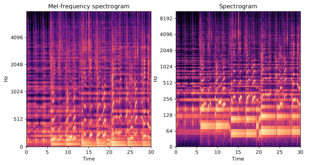
2.1. Visual Features

Researches show that it is difficult for people to perceive the frequency on a linear scale. Compared with the high-frequency domain, human beings are better at distinguishing the low-frequency domain. For example, humankind can easily differentiate the variance between 500 Hz and 1000 Hz, but find it hard to sense the difference between 10,000 Hz and 10,500 Hz, even though the two pairs have the same span. The Mel scale is a perceptual scale of pitches judged by listeners to be equal in distance from one to another. Stanley Smith Stevens, John Volkman, and Newman named it [30] based on the definition of frequency. The following is an approximate mathematical conversion between the Mel scale and the linear frequency scale hertz:

$$Mel\left(f\right)=2595\times lg(1+\frac{f}{700}).$$

(1)

Then, the energy spectrum needs to pass through a set of Mel scale triangular filter banks (as shown in Figure 1) to get the Mel-frequency spectrogram. The frequency loudness of the triangular filter is defined as:

$$H_m\left(k\right)=\left\{\begin{array}{c}0,k\le f(m-1)\hfill \\ \frac{2(k-f(m-1\left)\right)}{\left(f\right(m+1)-f(m-1\left)\right)\left(f\right(m)-f(m-1\left)\right)},f(m-1)\le k\le f\left(m\right)\hfill \\ \frac{2\left(f\right(m+1)-k)}{\left(f\right(m+1)-f(m-1\left)\right)\left(f\right(m)-f(m-1\left)\right)},f\left(m\right)\le k\le f(m+1)\hfill \\ 0,k\ge f(m-1)\hfill \end{array}\right.$$

(2)

where ${\sum }_{m=0}^{M-1}{H}_m\left(k\right)=1$, the number of filters is M.

Figure 2 visualizes the Mel-frequency spectrogram and spectrogram, some extraordinary differences in the genre are captured, which means that the model we proposed can learn good visual features. A Mel-frequency spectrogram is a spectrogram where the frequencies are converted to the Mel scale and closely represents how humans perceive audio. The Mel scale is a scale for the measurement of psychological magnitude pitch [30]. It transforms the frequency scale so that sounds are at equal distances from each other. Therefore, a Mel-frequency spectrogram may be easier for the neural network to extract features from it. The y-axis (frequency) is mapped onto the Mel scale to form the Mel-frequency spectrogram. Then, the model extracts significant differences from the Mel-frequency spectrogram of each genre and conducts audio classification tasks based on autonomous learning. The window size is 2048, and the hop length is 512.

2.2. Audio Features

We choose nine audio features along different audio dimensions. Aside from the tempo feature, other features are extracted in the form of mean and variance. The window size of each frame is 2048, and the hop length is 512. This set of audio features (as shown in

Table 1. The set of audio features.

Timbral Texture Features	Other Features 1	Other Features 1
Chroma	Harmonic component	Tempo
Root Mean Square (RMS)	Percussive component
Spectral centroid
Spectral rolloff
Zero-Crossing Rate (ZCR)
MFCCs (1–20)

) provides the best results for our experiments.

2.2.1. Timbral Texture Features

The chroma feature is the general name of the chroma vector and chromatogram. The chroma vector contains 12 vector elements, representing the energy of 12 tones in a period (such as a frame). The same tone level energy of different octaves is accumulated, and the chromatogram is the sequence of the chroma vectors.

The spectral centroid [31] represents the position of the “centroid” of the sound and contains important information about the frequency distribution and energy distribution of the sound signal. It is calculated based on the weighted average of the sound frequency. Compared with the same length of blues songs, the frequency distribution of metal songs is denser toward the end. So, the spectral centroid of blues songs will be in the middle of the spectrum, while the spectral centroid of metal songs will be near the end of the spectrum. Spectral roll-off is a measurement of the shape of a signal, which represents the frequency as a specific percentage of spectral energy (such as 85%).

MFCCs of the signal are sets of 20 features, which can simply describe the overall shape of the spectral envelope and model speech features. ZCR reflects the times of signal crossing zero and the frequency characteristics. That is the number of times the speech signal changes from positive to negative or from negative to positive in each frame. This feature has been widely used in speech recognition and music information retrieval, and it is usually of higher value for high-impact sounds such as metal and rock. RMS value is the effective value of the total waveform. It is the area under the curve. In audio, it represents the amount of energy in the waveform. The peak value of the waveform is averaged into the total loudness, which is a more persistent amount than the rapidly changing volume.

2.2.2. Other Features

Tempo, which means “beats per minute”, is a unit of speed. The content and style of music determine the playing speed of music, which can be roughly divided into three categories: slow, medium, and fast. It is an important index to describe the content of music rhythm, which affects individuals’ music experience. The typical tempo range of hip-hop is 60–100 bpm, and between 115 and 130 bpm for house music.

Generally speaking, many sounds are composed of two elements: harmonic or percussive components. Harmonic components are the ones that we perceive to have a certain pitch. Percussive components often stem from the collision of two objects. Percussion has no pitch feature, but it has a clear location in time. The above two kinds of components provide the harmonic [32] feature and percussive [33] feature, respectively.

3. Proposed Design and Approach

This paper discusses the influence of learning feature interaction between different branches and layers on the final classification results in the multi-feature model. Considering that a Mel-frequency spectrogram is still an image, the model uses a CRNN structure for visual feature extraction. For audio feature combination, the model uses a direct and effective DNN structure for audio feature extraction. Thus, the model consists of a VFE module, an AFE module, and a classifier.

We mainly refer to the parameter settings in papers [22,23,24,25,26,27,28]. Then, based on the references, a random search determines the hyper-parameters of the model. We will provide a statistical distribution for each hyper-parameter. For each iteration, the random search will set the hyper-parameters by sampling the distribution defined above. The sampled hyper-parameters yield a model. The classification accuracy of the model is evaluated through 10-fold cross-validation. Finally, the best hyper-parameter combination is selected to form the final model.

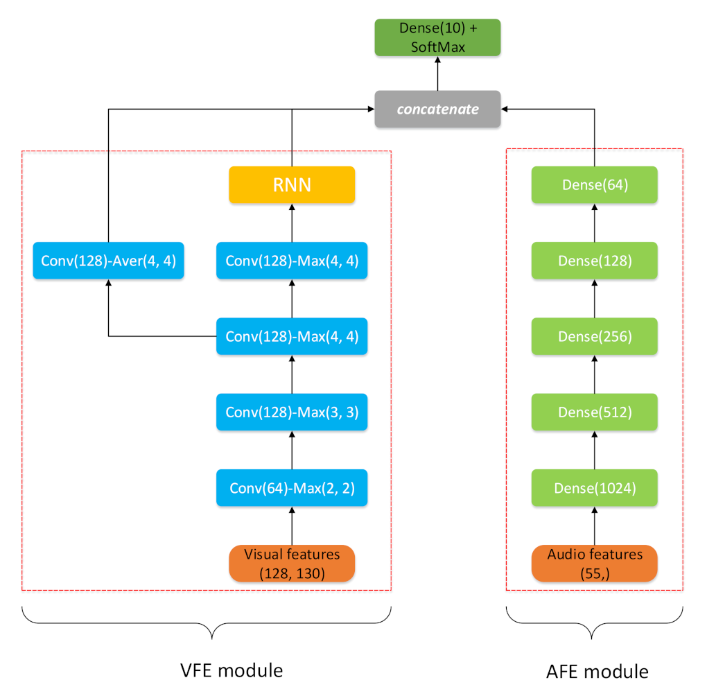
3.1. The Visual Features Extractor (VFE) Module

Based on the CRNN model [24], the VFE module uses parallel convolution to optimize. It includes 3-layer two-dimensional convolution (as shown in Figure 3), 1-layer parallel convolution, and 2-layer RNN. For parallel convolution, one branch output uses max-pooling, and the other uses average-pooling. The beneficial aspect is that it provides more statistical information for the following layers and further enhances the recognition ability of the model.

In each convolution operation process, except the first convolution layer has 64 different kernels of equal size, the other convolution layers have 128 kernels. The size of each convolution kernel is 3 × 3, and the hop length is 1. Furthermore, each convolution kernel forms a mapping relationship with all the underlying features. The convolution kernel is covered at the corresponding position of the input. Multiply each value in the convolution kernel and the value of the corresponding pixel in the input. Furthermore, the sum of the above products is the value of the target pixel in the output. Repeat this operation for all positions of the input. After each convolution, the Batch Normalization (BN) [34] and Rectified Linear Unit (ReLU) operations are implemented. We also add a max-pooling layer (which only works on one branch of parallel convolution layers) to reduce the parameters. Furthermore, it helps the model to expand the receptive field and achieve non-linearly. The filter sizes of pooling operations mainly adopt 2 × 2 with stride 2, 3 × 3 with stride 3 for the first and second pooling operations separately, 4 × 4 with stride 4 for the others. The function of the convolution layer and pooling layer is to map the original data to the hidden layer feature space.

The VFE module uses 2-layer RNNs with Gated Recurrent Units (GRU) to summarize temporal patterns on the top of two-dimensional 3-layer convolutions and 1-layer parallel convolutions (as shown in Figure 4). Considering that humans may pay more attention to a prominent rhythm when recognizing the music genre, only the branch output of parallel convolution using max-pooling operation is put into RNNs. Instead of simply adding outputs together, we concatenate the output of RNNs and the branch output of parallel convolution (which uses an average-pooling operation) to avoid losing some information. Then, we get a vector with a length of 160.

3.2. The Audio Features Extractor (AFE) Module

The AFE module consists of five dense layers. The size of each is 1024, 512, 256, 128, and 64. We use the ReLU as an activation function and then execute BN transform immediately to regularize our model. A dropout layer of 0.4 is added after each BN layer [35] to alleviate the over-fitting problem in the experiment. Finally, the AFE module will output a vector with a length of 64.

3.3. Network Structure

As shown in Figure 4, the VFE module, AFE module, and classifier constitute the whole network model. In particular, the model in Figure 4 is a benchmark model to measure the excellence of our method, and we call it the original model in the following. Finally, we concatenate the outputs of the two modules to form an eigenvector with a length of 224. Fully Connected (FC) layers usually play the role of “Classifier” in the whole neural network. However, in this paper, we only use one FC layer with SoftMax function for classification to reduce the parameters. It is easier to interpret the correspondence between feature maps and genres and less prone to over-fitting than traditional multi-layer fully connected layers. Since the last layer uses the SoftMax function, we will get the probability distribution. In general, the SoftMax function is defined as:

$$\delta {\left(z\right)}_j=\frac{e^{z_j}}{{\sum }_{k-1}^K{e}^{z_k}}$$

(3)

3.4. Middle-Level Learning Feature Interaction Method

One-way interaction (audio) mode: The model shown in Figure 5 is in one-way interaction (audio) mode. Visual learning features play a complementary role in this mode. The output in the VFE module and the output of the dense layer in the AFE module are concatenated and then put into the upper dense layer for training. In this mode, the VFE module provides two kinds of learning features: A (visual learning features obtained through RNN layer) and B (add the visual learning feature of Conv-Aver layer based on A). According to these two learning features, one-way interaction (audio) mode is divided into one-way interaction sub-mode A and one-way interaction sub-mode B. The audio feature extraction module provides four learning features in different layers, thus forming four connection paths: (1, 1’), (2, 2’), (3, 3’), (4, 4’). In particular, the above connection paths have a feature. For example, connection paths 1 and 1’ cannot exist simultaneously in the current mode.

One-way interaction (vision) mode: The model shown in Figure 6 is in one-way interaction (vision) mode. Audio learning features play a complementary role in this mode. The output of the dense layer in the AFE module and the output of the fourth Conv-Max layer are concatenated and then put into the RNN layer for training. In this mode, the audio feature extraction module provides five learning features on different layers, thus forming five connection paths: a, b, c, d, and e.

Two-way interaction mode: The two-way interaction mode is a combination of the above two one-way interaction modes. The AFE module can provide four audio learning features, and the corresponding paths are b, c, d, and e. Generally speaking, we can get eight different situations in this mode. For easier description, according to the two learning features provided by the VFE module, we divide the two-way interaction mode into two-way interaction sub-mode A and two-way interaction sub-mode B.

4. Experimental Setup and Results

4.1. Dataset

G. Tzanetakis and P. Cook collected the GTZAN dataset [36] for their well-known paper on music genre classification tasks [37]. The dataset has ten genres, including blues, classical, country, disco, hip-hop, jazz, metal, pop, reggae, rock, and 100 songs per genre. Each file is sampled at 22,050 Hz, 16 bits, and then stored in a 30-s monophonic .wav format. Although the dataset is small and old, it still widely serves as a benchmark in academia.

4.2. Preprocessing

First of all, load the audios as source data and split them into a nearly 3-s window [22]. Specifically, 66,149 sampling points are reserved every three seconds, and fragments with insufficient length will be discarded. This step can increase the amount of data and simplify the transformation process (such as the Mel-frequency spectrogram). At the same time, to make the model learn the characteristics of each genre better, the data sequence is scrambled after the dataset is segmented. Experiments show that this is very important.

Table 2. GTZAN Dataset Description.

Genre	Tracks	Number of Clips
Reggae	100	1000
Metal	100	1000
Pop	100	1000
Jazz	100	1000
Blues	100	1000
Disco	100	999
Rock	100	998
Classical	100	998
Hip-hop	100	998
Country	100	997
Total	1000	9990

shows the GTZAN dataset description.

As for the input of the VFE module, the Librosa library is used to extract Mel-frequency spectrograms, which contain about 130 frames each, and each has 128 Mel-filter bands. A set of 55 audio features are put into the AFE module, setting a frame length of 2048 with a 25% overlap.

4.3. Training and Other Details

All files in the GTZAN dataset are transformed to Mel-frequency spectrograms and audio features separately by the preprocessing program presented in Section 4.2: the Mel-frequency spectrogram with size 128 × 130 input to the VFE module and the audio features with the size 55 × 1 input to the AFE module.

For the choice of hyper-parameters, we refer to the experimental results of many academic papers and industry standards. For example, in the first convolution layer of the VFE module, the kernel size is set to 3 × 3. We make some other minor adjustments by referring to other papers and specific examples to meet our special data requirements. For example, since the dataset we used is small, we choose to split it into training, validation, and test sets with the ratio of 7/2/1, rather than the ratio of 8/1/1 used in many papers [22,23,25]. At the same time, instead of using a 3-s window with an overlap rate of 50% at the beginning [22,23], we choose a 3-s window with an overlap rate of 0 according to the classification accuracy, running time, and data volume. In the process of experimental training, the cross-entropy loss function is applied to the last dense layer (which uses the SoftMax function) to make its value as small as possible. Cross-entropy mainly describes the distance between the actual value and the expected output. The smaller the value of cross-entropy is, the closer the two probability distributions are. Suppose that the probability distribution p is the expected output, the probability distribution q is the actual value, $H(p,q)$ is the cross-entropy, and let P and Q be probability density functions of p and q concerning r, then

$$H(p,q)=-\sum _{x\in X}p\left(x\right)log\left(q\left(x\right)\right)=-{\int }_{X}P\left(x\right)logQ\left(x\right)dr\left(x\right)$$

(4)

The optimizer we used is Adam with a default learning rate of 0.01 [25]. If the initial learning rate is set too small, the network convergence will be very slow, which will increase the time to find the optimal value. In addition, it is likely to converge into the local extremum, and cannot find the global optimal solution. Kingma and Lei Ba proposed the Adam optimizer, which combines the advantages of the Adaptive Gradient Algorithm (AdaGrad) and Root Mean Square Prop (RMSProp) [38]. The optimizer can deal with sparse gradient better, that is, the gradient is 0 at many steps. With Adam, our models trained more quickly and did not plateau as early. Furthermore, our model uses the ReduceLROnPlatrau() function to decrease the learning rate when the standard estimate stops improving. The model has trained over 150 epochs and is adapted in each with a mini-batch size of 128 instances.

Metric: The classification accuracy is evaluated through 10-fold cross-validation [39,40] across all experiments to get more accurate results. Classification accuracy is the ratio of the number of correct predictions to the total number of input samples. It works well only if the number of samples belonging to each class is equal. Considering that the number of samples used in this paper is the same, this paper takes classification accuracy as the standard to measure the classification results. We balance the number of songs for each genre in training, validation, and test sets. Finally, the total classification accuracy is the average of 10-fold cross-validations.

Experiment Platform: We use the Keras [41] and TensorFlow [42] library to build our model in python. Librosa library is used to process audio data. All the experiments are done on Google’s Colaboratory platform.

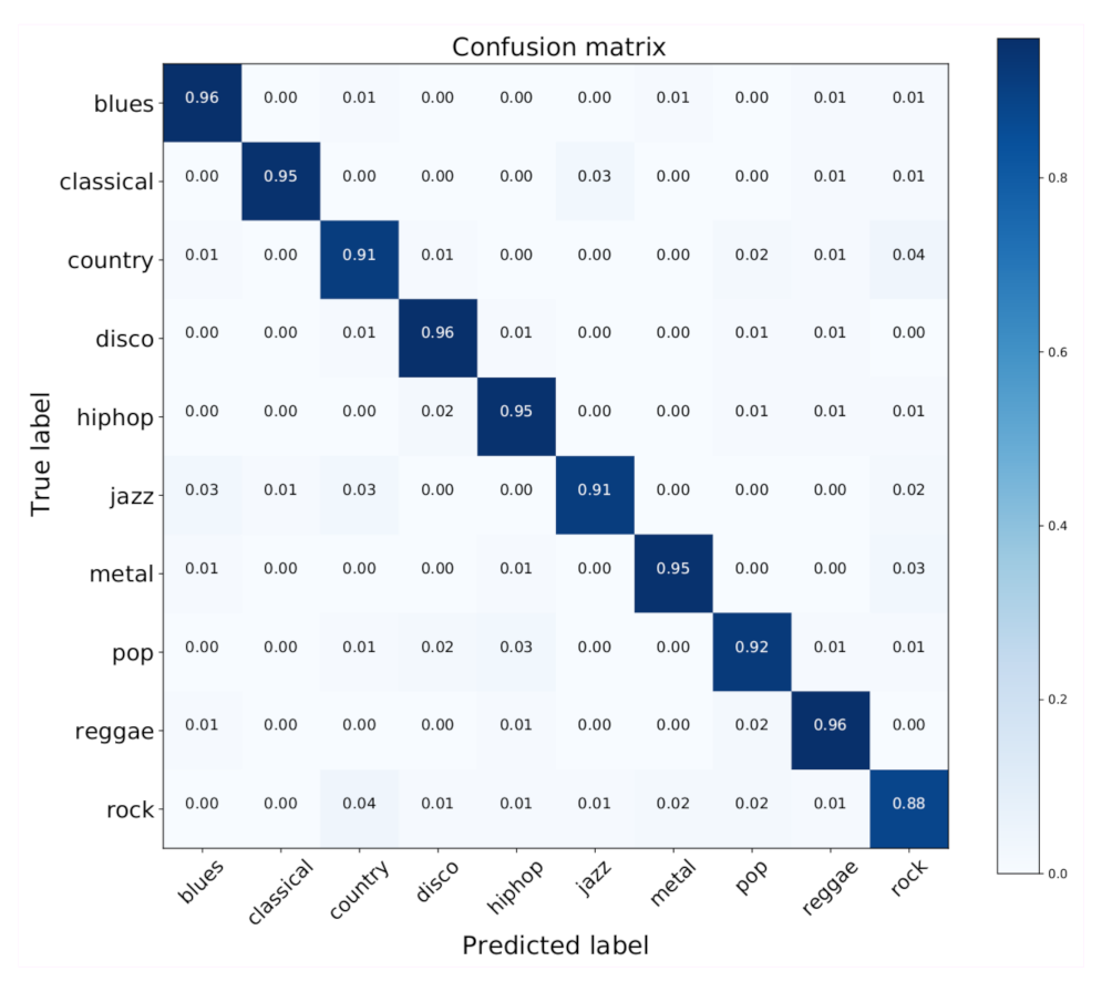
4.4. Classification Results on GTZAN

4.4.1. Classification Results of One-Way Interaction (Audio) Mode

As is shown in Figure 5, the network topology in one-way interaction (audio) mode includes two sub-modes. The VFE module provides two visual learning features. The AFE module provides four audio learning features. To further distinguish, we use the number of filters in the dense layer to mark. The experimental results in

Table 3. The experimental results of one-way interaction (audio) mode. If the path label is marked with “[ ]”, it means that the path implements the middle-level learning feature interaction method.

Learning Feature (A or B)	Paths	Dense Layer Marker	Accuracy (%)
A	[1] 2’ 3’ 4’	1024	92.35
A	1’ [2] 3’ 4’	512	92.18
A	1’ 2’ [3] 4’	256	92.60
A	1’ 2’ 3’ [4]	128	93.14
			Avg: 92.5675
B	[1] 2’ 3’ 4’	1024	93.65
B	1’ [2] 3’ 4’	512	91.08
B	1’ 2’ [3] 4’	256	91.67
B	1’ 2’ 3’ [4]	128	93.28
			Avg: 92.42

contain eight different situations of the above learning features. In particular, sub-mode B concatenates the output of the Conv-Avg block based on sub-mode A. The experimental results of the two sub-modes are analyzed. The highest accuracy of sub-mode A is 93.14%, and the average accuracy is 92.5675%. The highest accuracy of sub-mode B is 93.65%, and the average accuracy is 92.42%. Compared with the experimental results of sub-mode A, the classification effect of sub-mode B has been improved visibly for the two cases of dense (1024 and 128). Considering that sub-mode B contains more learning features, people may think that the more interactive information they feel, the more sufficient learning features, the better the classification effect. However, for other cases, the classification result of sub-mode B decreases. Therefore, we can know that using more learning features as interactive information may produce a gain effect or inhibit other learning features from playing a role.

4.4.2. Classification Results of One-Way Interaction (Vision) Mode

The network topology in one-way interaction (video) mode is shown in Figure 6. Due to the limitation of the model itself, we only consider one visual learning feature of the VFE module. The AFE module provides five audio learning features. The experimental results in

Table 4. The experimental results of one-way interaction (vision) mode.

Input Size of RNN	Paths	Dense Layer Marker	Accuracy (%)
(72, 16)	e	1024	93.11
(40, 16)	d	512	91.99
(24, 16)	c	256	91.28
(16, 16)	b	128	91.79
(16, 12)	a	64	91.72
			Avg: 91.978

include five situations composed of the above learning features. The highest accuracy is 93.11%, and the average accuracy is 91.66%. Compared with the two sub-modes of the one-way interaction (audio) mode, the improvement of the classification effect of this mode is not distinct. The experimental results declare that different learning features as supplementary information have different roles in the classification results.

4.4.3. Classification Results of Two-Way Interaction Mode

Because the two one-way interaction modes have good performance in the classification task, we want to explore whether the combination of the two one-way modes can further improve the classification effect of the model. Since dense (64) is the last layer of the feature extractor, the AFE module provides only four audio learning features. Since the VFE module provides two learning features A and B, the two-way interaction mode also includes two sub-modes. For ease of expression, we use A and B to represent the two sub-modes. As shown in

Table 5. The experimental results of two-way interaction mode.

Learning Feature (A or B)	Paths	Dense Layer Marker	Accuracy (%)
A	[1] 2’ 3’ 4’ e	1024	93.01
A	1’ [2] 3’ 4’ d	512	90.79
A	1’ 2’ [3] 4’ c	256	92.74
A	1’ 2’ 3’ [4] b	128	92.82
			Avg: 92.39
B	[1] 2’ 3’ 4’ e	1024	92.84
B	1’ [2] 3’ 4’ d	512	92.72
B	1’ 2’ [3] 4’ c	256	93.04
B	1’ 2’ 3’ [4] b	128	93.28
			Avg: 92.97

, the highest accuracy of two-way interaction sub-mode A is 93.01%, and the average accuracy is 92.39%. However, the worst classification result of dense (256) is 90.79%. The highest accuracy of two-way interaction sub-mode B is 93.28%, and the average accuracy is 92.97%, which is the highest average classification accuracy.

On the one hand, although the two-way interaction sub-mode A has more learning features than one-way interaction, its average accuracy is lower than other modes. This situation shows that more learning features as interactive information may inhibit other learning features from playing a role. On the other hand, two-way interaction sub-mode B is established based on two-way interaction sub-mode A, but it has the highest average accuracy. This situation further verifies that more learning features as interactive information may have a gain effect. Therefore, the combination of the two one-way interaction modes can improve the classification effect to a certain extent. However, the final classification result is not the sum of the learning feature effects of two one-way interaction modes. Furthermore, the role of the learning feature in one mode depends on the value of the learning feature in the other mode. The key to getting better classification results is to find the appropriate way and model structure.

4.4.4. Comparison of Each Mode

As can be seen from the above, the classification accuracy of the original model is 90.67%. We can see intuitively from Figure 7 that the classification results of all modes are better than the original model. The results prove the effectiveness of the proposed method. By observing the classification accuracy of the five modes under different dense layer markers, we can see that the classification accuracy of all modes is high at both ends and low in the middle. It shows that the middle-level learning feature interaction method to the layer close to the input and output of the model can improve the classification effect more effectively than other layers. As for why the optimal results often appear at both ends, we get the following two possible reasons:

• Considering that dense (128) is closer to the output layer and has a similar degree of abstraction with the input and output of the RNN layer, the restriction between the two learning features will be smaller, and the gain effect will be more prominent.
• Considering that dense (1024) is closer to the input layer, it is equivalent to increasing the depth of the model for the input and output of RNN, which is conducive to extracting more effective learning features.

From Figure 8, we can see that all the modes have good classification performance in the four genres of blues, disco, metal, and reggae. The classification accuracy of country, pop, and rock is low. On the one hand, we can speculate that the middle-level learning feature method still has limitations, which can not effectively classify some genres. On the other hand, we can also infer that these genres have great similarities in audio and video features.

The classification accuracy is regarded as the primary metric to measure the quality of the model. A confusion matrix is used to visualize model performance, with each column representing the predicted value and each row representing the actual category. All the correct predictions are on the diagonal, so it is easy to see where the errors are from the confusion matrix because they are all off the diagonal. The confusion matrix allows us to do more analysis than just get the precision and recall values.

As shown in Figure 8, none of the modes can effectively classify the three genres of country, pop, and rock. We analyze the optimal confusion matrix in the one-way interaction (audio B) mode shown in Figure 9. This mode only correctly classifies 90% of country music and wrongly classifies the other 10% as pop and rock. The classification accuracy of pop music is 92%, and most misclassifications identify the music as hip-hop and disco. Rock music classification accuracy is the lowest at only 88%. A large number of them are classified as country, metal, and pop. On the one hand, we can infer that this music has many similarities in its visual and audio characteristics. On the other hand, rock music has indeed influenced many other types of music throughout history.

4.4.5. Comparison to State-of-the-Art

In

Table 6. Classification accuracy(%) on GTZAN dataset is compared across recently proposed methods. In particular, SSD is Statistical Spectrum Descriptor.

Methods	Preprocessing	Accuracy (%)
CRNN [24]	mel-spectrogram	86.5
Hybrid model [43]	MFCCs, SSD, etc.	88.3
Combining Visual Furthermore, Acoustic (CVAF) [26]	mel-spectrogram, SSD, etc.	90.9
Music Feature Maps with CNN (MFMCNN) [27]	STFT, ZCR, etc	91.0
Multi-DNN [28]	MFCCs	93.4
BBNN [25]	mel-spectrogram	93.7
Ours(one-way interaction)	mel-spectrogram, ZCR, etc.	93.65

, we compare our method with previous excellent results on the GTZAN dataset. Experimental results show that the best classification accuracy of the method (one-way interaction (audio) mode) on the GTZAN dataset is 93.65% (10 folds cross-validation), which reaches the state-of-the-art performance of the current GTZAN dataset. Our classification result is slightly worse than 93.7% of the BBNN. However, considering that BBNN is composed of multiple Inception blocks, it needs a tremendous number of convolution operations. As shown in

Table 7. Comparison of training speed.

Methods	Graphics Processing Unit (GPU)	Compute Capability	Run Time/Epoch
BBNN	NVIDIA Titan XP (12 GB)	6.1	28 s
ours	NVIDIA Tesla K80 (12 GB)	3.7	19 s

, our method is much faster than BBNN.

5. Conclusions

This paper proposes a middle-level learning feature interaction method using deep learning. The method aims to solve the problem that the branches of a multi-feature model in the existing music genre classification methods are relatively independent and not interactive, resulting in the lack of learning features for music genre classification. The classification results of each mode are better than the original network architecture. Furthermore, we have shown how our method is effective by comparing state-of-the-art methods. Furthermore, the experimental results prove that the final classification result is not the total sum of the learning feature effects. Using more learning features as interactive information may produce a gain effect or inhibit other learning features from playing a role. Besides, the classification results of all modes show that the learning features near the input and output have a better gain effect on improving the classification results. The above conclusions prove that the proper use of the middle-level learning features interaction method in a multi-feature model can effectively promote the gain effect between different learning features and improve the classification results.

In the future, we will try new methods, such as adopting acoustic features (e.g., SSD, Rhythm Histogram (RH)) as the input of the model or fusing attention mechanisms to give neural networks the ability to focus on their input subset. Meanwhile, we will also research how to distinguish those genres with similar spectral characteristics.

References

1. Song, Y.; Zhang, C. Content-based information fusion for semi-supervised music genre classification. IEEE Trans. Multimed. 2007, 10, 145–152. [Google Scholar] [CrossRef]
2. Fu, Z.; Lu, G.; Ting, K.M.; Zhang, D. A survey of audio-based music classification and annotation. IEEE Trans. Multimed. 2010, 13, 303–319. [Google Scholar] [CrossRef]
3. Lim, S.-C.; Lee, J.-S.; Jang, S.-J.; Lee, S.-P.; Kim, M.Y. Music-genre classification system based on spectro-temporal features and feature selection. IEEE Trans. Consum. Electron. 2012, 58, 1262–1268. [Google Scholar] [CrossRef]
4. Lee, C.-H.; Shih, J.-L.; Yu, K.-M.; Lin, H.-S. Automatic music genre classification based on modulation spectral analysis of spectral and cepstral features. IEEE Trans. Multimed. 2009, 11, 670–682. [Google Scholar]
5. Liu, J.; Yin, T.; Cao, J.; Yue, D.; Karimi, H.R. Security control for TS fuzzy systems with adaptive event-triggered mechanism and multiple cyber-attacks. IEEE Trans. Syst. Man Cybern. Syst. 2020, 1–11. [Google Scholar] [CrossRef]
6. Liu, J.; Suo, W.; Xie, X.; Yue, D.; Cao, J. Quantized control for a class of neural networks with adaptive event-triggered scheme and complex cyber-attacks. Int. J. Robust Nonlinear Control 2021, 31, 4705–4728. [Google Scholar] [CrossRef]
7. Liu, J.; Wang, Y.; Zha, L.; Xie, X.; Tian, E. An event-triggered approach to security control for networked systems using hybrid attack model. Int. J. Robust Nonlinear Control 2021, 31, 5796–5812. [Google Scholar] [CrossRef]
8. Jin, K.H.; McCann, M.T.; Froustey, E.; Unser, M. Deep convolutional neural network for inverse problems in imaging. IEEE Trans. Image Process. 2017, 26, 4509–4522. [Google Scholar] [CrossRef] [PubMed] [Green Version]
9. Zhang, K.; Zuo, W.; Chen, Y.; Meng, D.; Zhang, L. Beyond a gaussian denoiser: Residual learning of deep CNN for image denoising. IEEE Trans. Image Process. 2017, 26, 3142–3155. [Google Scholar] [CrossRef] [Green Version]
10. Badrinarayanan, V.; Kendall, A.; Cipolla, R. SegNet: A deep convolutional encoder-decoder architecture for image segmentation. IEEE Trans. Pattern Anal. Mach. Intell. 2017, 39, 2481–2495. [Google Scholar] [CrossRef]
11. Ren, S.; He, K.; Girshick, R.; Sun, J. Faster R-CNN: Towards real-time object detection with region proposal networks. IEEE Trans. Pattern Anal. Mach. Intell. 2017, 39, 1137–1149. [Google Scholar] [CrossRef] [Green Version]
12. Deng, X.; Zhang, Y.; Xu, M.; Gu, S.; Duan, Y. Deep coupled feedback network for joint exposure fusion and image super-resolution. IEEE Trans. Image Process. 2021, 30, 3098–3112. [Google Scholar] [CrossRef]
13. Qian, Y.; Chen, Z.; Wang, S. Audio-visual deep neural network for robust person verification. IEEE/ACM Trans. Audio Speech Lang. Process. 2021, 29, 1079–1092. [Google Scholar] [CrossRef]
14. Luo, Y.; Mesgarani, N. Conv-tasNet: Surpassing ideal time–frequency magnitude masking for speech separation. IEEE/ACM Trans. Audio Speech Lang. Process. 2019, 27, 1256–1266. [Google Scholar] [CrossRef] [PubMed] [Green Version]
15. Abdel-Hamid, O.; Mohamed, A.; Jiang, H.; Deng, L.; Penn, G.; Yu, D. Convolutional neural networks for speech recognition. IEEE/ACM Trans. Audio Speech Lang. Process. 2014, 22, 1533–1545. [Google Scholar] [CrossRef] [Green Version]
16. Dethlefs, N.; Schoene, A.; Cuayáhuitl, H. A divide-and-conquer approach to neural natural language generation from structured data. Neurocomputing 2021, 433, 300–309. [Google Scholar] [CrossRef]
17. Zhang, K.; Sun, S. Web music emotion recognition based on higher effective gene expression programming. Neurocomputing 2013, 105, 100–106. [Google Scholar] [CrossRef]
18. Zhang, J.; Huang, X.; Yang, L.; Nie, L. Bridge the semantic gap between pop music acoustic feature and emotion: Build an interpretable model. Neurocomputing 2016, 208, 333–341. [Google Scholar] [CrossRef]
19. Wu, M.-J.; Jang, J.-S.R. Combining acoustic and multilevel visual features for music genre classification. ACM Trans. Multimed. Comput. Commun. Appl. 2015, 12, 1–17. [Google Scholar] [CrossRef]
20. Montalvo, A.; Costa, Y.M.G.; Calvo, J.R. Language identification using spectrogram texture. In Iberoamerican Congress on Pattern Recognition; Springer: Berlin, Germany, 2015; pp. 530–550. [Google Scholar]
21. Hafemann, L.G.; Oliveira, L.S.; Cavalin, P. Forest species recognition using deep convolutional neural networks. In Proceedings of the 2014 22Nd International Conference on Pattern Recognition, Stockholm, Sweden, 24–28 August 2014; pp. 1103–1107. [Google Scholar]
22. Zhang, W.; Lei, W.; Xu, X.; Xing, X. Improved music genre classification with convolutional neural networks. In Proceedings of the Interspeech, San Francisco, CA, USA, 8–12 September 2016; pp. 3304–3308. [Google Scholar]
23. Yang, H.; Zhang, W.-Q. Music genre classification using duplicated convolutional layers in neural networks. In Proceedings of the Interspeech, Graz, Austria, 15–19 September 2019; pp. 3382–3386. [Google Scholar]
24. Choi, K.; Fazekas, G.; Sandler, M.; Cho, K. Convolutional recurrent neural networks for music classification. In Proceedings of the 2017 IEEE International Conference on Acoustics, Speech and Signal Processing (ICASSP), New Orleans, LA, USA, 5–9 March 2017; pp. 2392–2396. [Google Scholar]
25. Liu, C.; Feng, L.; Liu, G.; Wang, H. Bottom-up broadcast neural network for music genre classification. Multimed. Tools Appl. 2021, 80, 7313–7331. [Google Scholar] [CrossRef]
26. Nanni, L.; Costa, Y.M.; Lucio, D.R.; Silla, C.N., Jr.; Brahnam, S. Combining visual and acoustic features for audio classification tasks. Pattern Recognit. Lett. 2017, 88, 49–56. [Google Scholar] [CrossRef]
27. Senac, C.; Pellegrini, T.; Mouret, F.; Pinquier, J. Music feature maps with convolutional neural networks for music genre classification. In Proceedings of the 15th International Workshop on Content-Based Multimedia Indexing, Florence, Italy, 19–21 June 2017; pp. 1–5. [Google Scholar]
28. Dai, J.; Liu, W.; Ni, C.; Dong, L.; Yang, H. “Multilingual” deep neural network For music genre classification. In Proceedings of the Sixteenth Annual Conference of the International Speech Communication Association, Stockholm, Sweden, 20–24 August 2017. [Google Scholar]
29. He, K.; Zhang, X.; Ren, S.; Sun, J. Deep residual learning for image recognition. In Proceedings of the IEEE Conference on Computer Vision and Pattern Recognition, Las Vegas, NV, USA, 27–30 June 2016; pp. 770–778. [Google Scholar]
30. Stevens, S.S.; Volkmann, J.; Newman, E.B. A scale for the measurement of the psychological magnitude pitch. J. Acoust. Soc. Am. 1937, 8, 185–190. [Google Scholar] [CrossRef]
31. Klapuri, A.; Davy, M. Signal Processing Methods for Music Transcription; Springer Science & Business Media: Berlin/Heidelberg, Germany, 2007; pp. 45–68. [Google Scholar]
32. Papadopoulos, H.; Peeters, G. Local key estimation from an audio signal relying on harmonic and metrical structures. IEEE Trans. Audio Speech Lang. Process. 2011, 20, 1297–1312. [Google Scholar] [CrossRef]
33. Lim, W.; Lee, T. Harmonic and percussive source separation using a convolutional auto encoder. In Proceedings of the 2017 25th European Signal Processing Conference (EUSIPCO), Kos, Greece, 28 August–2 September 2017; pp. 1804–1808. [Google Scholar]
34. Ioffe, S.; Szegedy, C. Batch normalization: Accelerating deep network training by reducing internal covariate shift. In Proceedings of the International Conference on Machine Learning, Lille, France, 6–11 July 2015; pp. 448–456. [Google Scholar]
35. Gupta, S. GTZAN Dataset—Music Genre Classification. 2021. Available online: https://www.kaggle.com/imsparsh/gtzan-genre-classification-deep-learning-val-92-4 (accessed on 21 March 2021).
36. Tzanetakis, G.; Cook, P. Marsyas “Data Sets”. GTZAN Genre Collection. 2002. Available online: http://marsyas.info/download/data_sets (accessed on 21 March 2021).
37. Tzanetakis, G.; Cook, P. Musical genre classification of audio signals. IEEE Trans. Speech Audio Process. 2002, 10, 293–302. [Google Scholar] [CrossRef]
38. Kingma, D.P.; Ba, J. Adam: A method for stochastic optimization. In Proceedings of the 3rd International Conference on Learning Representations (ICLR), San Diego, CA, USA, 7–9 May 2015. [Google Scholar]
39. Browne, M.W. Cross-Validation Methods. J. Math. Psychol. 2000, 44, 108–132. [Google Scholar] [CrossRef] [Green Version]
40. Sylvain, A.; Alain, C. A Survey of Cross-Validation Procedures for Model Selection. Stat. Surv. 2010, 4, 40–79. [Google Scholar]
41. Francois, C. Keras. 2015. Available online: https://keras.io. (accessed on 21 March 2021).
42. Abadi, M.; Agarwal, A.; Barham, P.; Brevdo, E.; Chen, Z.; Citro, C.; Corrado, G.S.; Davis, A.; Dean, J.; Devin, M.; et al. Tensorflow: Large-scale machine learning on heterogeneous distributed systems. arXiv 2016, arXiv:1603.04467. [Google Scholar]
43. Karunakaran, N.; Arya, A. A scalable hybrid classifier for music genre classification using machine learning concepts and spark. In Proceedings of the 2018 International Conference on Intelligent Autonomous Systems (ICoIAS), Singapore, 1–3 March 2018; pp. 128–135. [Google Scholar]
Figure 1. Mel scale filter banks.
Electronics 10 02206 g001
Figure 2. Mel-frequency spectrogram and Spectrogram.
Electronics 10 02206 g002
Figure 3. Convolution block. In order to simplify the network representation, each convolution block contains four different layers. Convolution blocks are divided into two types according to different pooling operations: Conv-Max block and Conv-Aver block. The dropout ratio is set to 0.1 [24]. In particular, BN is Batch Normalization.
Electronics 10 02206 g003
Figure 4. The original network architecture. It is a benchmark model to evaluate the effectiveness of middle-level learning feature interaction method.
Electronics 10 02206 g004
Figure 5. The network architecture using one-way (audio) interaction.
Electronics 10 02206 g005
Figure 6. The network architecture using one-way (visual) interaction.
Electronics 10 02206 g006
Figure 7. Accuracy comparison of each mode.
Electronics 10 02206 g007
Figure 8. Comparison of optimal accuracy of each mode.
Electronics 10 02206 g008
Figure 9. Optimal confusion matrix of one-way interaction (audio B) mode.
Electronics 10 02206 g009