Robust Asynchronous H_∞ Observer-Based Control Design for Discrete-Time Switched Singular Systems with Time-Varying Delay and Sensor Saturation: An Average Dwell Time Approach

Abstract

This work discuss the robust stabilization problem for discrete-time switched singular systems with simultaneous presence of time-varying delay and sensor nonlinearity. To this end, an observer-based controller was synthesized that works under asynchronous switching signals. Investigating the average dwell time approach and using a Lyapunov–Krasovskii functional with triple sum terms, sufficient conditions were derived for achieving the existence of such asynchronous controller and guaranteeing the resulting closed-loop system to be exponentially admissible with $H_{\infty }$ performance level. Subsequently, the effectiveness of the proposed control scheme was verified through two numerical examples.

1. Introduction

Lately, great interest has been devoted to the study of switched singular systems on both theoretical and application fronts ([1,2,3], and the references therein). From a mathematical point of view, switched singular systems are typically each composed of a finite number of subsystems and a switching law that specifies the active subsystems at each instant of time. Each subsystem is defined by ordinary differential equations that describe the dynamical part in the system and algebraic equations that represent the interrelationships between different components in the system. Moreover, the switching law plays a crucial role in determining the dynamic behavior of switched singular systems [2,4,5]. All the montioned works are concerned with arbitrary switching signal to study switched singular systems. Therefore, many switched singular systems fail to preserve stability under switching signals of this kind, but may be stable under some prescribed switching signals. Thus, we devote our attention in this work on the ADT approach, which means that the number of switches in a finite interval is bounded and the average time between consecutive switching is not less than a specific constant [6,7].

It should be noted that time-delay occurrence represents, usually, a source of instability and poor performance of dynamic systems. As a result, the study of switched singular delayed systems has aroused considerable attention [8,9,10,11,12].

Furthermore, study of robustness against external disturbances is significant [13]. For this purpose, different techniques have been investigated to ensure robust stability. Thus, the $H_{\infty }$ technique has been used to study the problem of control [9,14] and filtering [4,15] for switched singular systems with time delay.

Nevertheless, all the previous works cited investigated only linear switched singular systems with synchronous switching modes between the respective controllers and systems. Generally, in practice the switching instants of the controllers exceed or lag behind those of the subsystems. Accordingly, it is necessary and more realistic to consider this phenomenon when dealing with control problems for switched singular systems. The asynchronous switched control problem covers many fields of application, such as Markovian jump systems [16], networked control systems [17] and neural systems [18,19]. To date, some appreciable studies have been reported for switched systems under asynchronous switching [20,21,22,23,24]. To the best of our knowledge, the stabilization problem for discrete-time switched singular time-delay systems under asynchronous switching has not been fully investigated, except in some works where the state feedback stabilization has been investigated for discrete-time singular systems [3,25], and for continuous singular systems [12,26]. That was the primary motivation for this work.

We note that all the methods suggested in the previous references suppose that the system state variables are available for measurements. However, the state variables for many real plants are mostly not fully accessible for many reasons, such as the non-existence of correct sensors to measure some states, or an increased number of sensors making the whole system more complex. Thus, the design of observers to estimate the system states is more reasonable. Accordingly, considerable attention has been paid to the observer-based control problem for switched singular systems. For example, in [27,28] the problem of observers design for a class of discrete-time switched singular systems subject to constant delay, unknown inputs and arbitrary switching sequences was considered. In addition, the robust $H_{\infty }$ non-fragile observer-based control issue for switched discrete singular systems with time-varying delays under arbitrary switching was treated in [29]. The authors in [30] studied the observer-based asynchronous $H_{\infty }$ control problem for switched singular systems with quadratically inner-bounded nonlinearity. A two step method was investigated in [31] to solve the problem of observer-based output-feedback asynchronous control design for a class of switched continuous-time Takagi–Sugeno fuzzy systems. Based on the singular value decomposition (SVD) technique and cone complementarity linearization (CCL) algorithm, the problem of asynchronous observer-based control for a class of discrete-time Markov jump systems has been treated in [32]. However, the SVD technique is difficult to use when the disturbance affects the measurements and the use of an iterative algorithm such the CCL can complicate the resolution of LMI conditions. In this regard, how to deal with dynamic systems with unavailable states for measurement by using an observer-based controller for the considered system under asynchronous switching was the second motivation for this work.

Due to many environmental circumstances, the actuator or sensor saturation can be interpreted as additive nonlinear exogenous disturbances. Thus, if such non-linearities are not considered in the controller design, the stability of system can be affected. Hence, in the analysis and implantation of the controller, the effect of non-linearity cannot be neglected [33,34,35,36]. Due to its theoretical and practical importance, some representative results regarding sensor saturation for switched systems have been considered [37,38,39]. However, the sensor saturation effect has not been investigated when dealing with the problem of asynchronous ADT observer-based control for discrete-time switched singular systems with time-varying delay. This represents the third motivation for this paper.

To study a general switched singular system from a practical point of view, it was assumed that the system under consideration consisted of unmeasured states, time-varying delay, and sensor saturation. The main contributions can be summarized as follows:

(i)

The switched singular systems were employed to cope with the problem of asynchronous observer-based control design using the ADT approach. Compared to [14,26,40,41], the design is considered to characterize dynamic systems with unavailable states for measurement, which closely reflects the reality with a more general structure.

(ii)

The exponential admissibility and $H_{\infty }$ performances of the switched singular systems were established by using an appropriate Lyapunov–Krasovskii functional with a triple-sum term. Delay-dependent LMI conditions were derived using the ADT approach.

(iii)

In contrast to [22,23,31], a one step method was developed to deal with the problem of asynchronous $H_{\infty }$ observer-based control design without considering any appropriate algorithm.

(iv)

Numerical examples were used to demonstrate the effectiveness of the proposed study.

An outline of this paper is given as follows. The system description and preliminaries are presented in Section 2. The main results, including the admissibility analysis and the asynchronous observer-based controller synthesis, are given in Section 3 and Section 4. A simulation example is illustrated in Section 5. Section 6 concludes the paper.

Notations. Throughout the paper, a real symmetric matrix $Y>0$$(Y\ge 0)$ denotes Y being a positive definite (or positive semi-definite) matrix. $sym\left(Y\right)$ stands for $Y+Y^T$. I and 0 symbolize the identity matrix and a zero matrix with appropriate dimensions, respectively. $Y\in {\mathbb{R}}^s$ denotes the $s-$ dimensional Euclidean space, and $Y\in {\mathbb{R}}^{s\times n}$ refers to the set of all $s\times n$ real matrices. ${\lambda }_{min}\left(P\right)$ and ${\lambda }_{max}\left(P\right)$ denote the minimum and maximum eigenvalues of P. In symmetric block matrices or long matrix expressions, we use a star * to represent a term that is induced by symmetry. Matrices, if their dimensions are not explicitly stated, are assumed to be compatible for algebraic operations. $\parallel .\parallel$ denotes the Euclidean norm of a vector and its induced norm of a matrix. $col\{Y,X\}$ denotes a column matrix.

2. System Description and Preliminaries

Consider a class of switched singular systems with time-varying delay described by

$$\begin{array}{cc}\hfill & \left\{\begin{array}{cc}\hfill Ex(k+1)& =A_{\sigma \left(k\right)}x\left(k\right)+A_{d\sigma \left(k\right)}x(k-d\left(k\right))+B_{1\sigma \left(k\right)}u\left(k\right)+B_{2\sigma \left(k\right)}w\left(k\right)\hfill \\ \hfill y\left(k\right)& =\phi \left(C_{\sigma \left(k\right)}x\left(k\right)\right)\hfill \\ \hfill z\left(k\right)& =C_{2\sigma \left(k\right)}x\left(k\right)+D_{\sigma \left(k\right)}w\left(k\right)\hfill \\ \hfill x\left(k\right)& =\varphi \left(k\right),k\in [-dM,0]\hfill \end{array}\right.\hfill \end{array}$$

(1)

where $u\left(k\right)\in {\mathbb{R}}^{m_u}$ is the control input vector, $z\left(k\right)\in {\mathbb{R}}^q$ is the controlled output vector, $x\left(k\right)\in {\mathbb{R}}^n$ is the state vector, $y\left(k\right)\in {\mathbb{R}}^p$ is the measured output, E is a singular matrix with $rank\left(E\right)<n$, and $\varphi \left(k\right)$ is a given initial condition sequence. The disturbance input vector, $w\left(k\right)\in {\mathbb{R}}^n$, is supposed to belong to $l_2[0,\infty )$. That is, ${\displaystyle \sum _{k=0}^{\infty }}{w}^T\left(k\right)w\left(k\right)<\infty$. $\sigma \left(k\right):$$[0,+\infty )$$\to \mathcal{I}=\{1,2\cdots ,N\}$ is a piecewise constant switching signal, with N being the number of subsystems.

Time-varying delay, $d\left(k\right)$, is defined as

$$0<d_m\le d\left(k\right)\le d_M$$

(2)

where $d_M$ and $d_m$, positive integers, represent the bounds of the delay.

Matrices E, $A_{\sigma \left(k\right)}$, $A_{d\sigma \left(k\right)}$, $B_{1\sigma \left(k\right)}$, $C_{\sigma \left(k\right)}$, $B_{2\sigma \left(k\right)}$, $C_{2\sigma \left(k\right)}$, and $D_{\sigma \left(k\right)}$ are constants with appropriate dimensions.

The saturation function $\phi \left(C_{\sigma \left(k\right)}x\left(k\right)\right)$ is an unknown nonlinear real-valued function which represents the sensor nonlinearity and satisfies:

$$\begin{array}{c}\hfill \begin{array}{cc}& {(\phi \left(\omega \right)-M_1\omega )}^T(\phi \left(\omega \right)-M_2\omega )\le 0\hfill \end{array}\end{array}$$

(3)

where $M_1\ge 0$ and $M_2\ge 0$ are diagonal matrices with $M_2>M_1$.

According to [42], the nonlinear function $\phi \left(C_{\sigma \left(k\right)}x\left(k\right)\right)$ can be decomposed into the following form:

$$\begin{array}{c}\hfill \begin{array}{cc}& \phi \left(C_{\sigma \left(k\right)}x\left(k\right)\right)={\phi }_n\left(C_{\sigma \left(k\right)}x\left(k\right)\right)+M_1{C}_{\sigma \left(k\right)}x\left(k\right)\hfill \end{array}\end{array}$$

(4)

where the nonlinearity ${\phi }_n\left(C_{\sigma \left(k\right)}x\left(k\right)\right)$ satisfies

$$\begin{array}{c}\hfill \begin{array}{cc}& {\phi }_n^T\left(C_{\sigma \left(k\right)}x\left(k\right)\right)\left[{\phi }_n\left(C_{\sigma \left(k\right)}x\left(k\right)\right)-M{C}_{\sigma \left(k\right)}x\left(k\right)\right] \le 0\hfill \end{array}\end{array}$$

(5)

where $M=M_2-M_1>0$

By considering the decomposition in (4), discrete-time switched singular systems (1) is formulated as:

$$\begin{array}{cc}\hfill & \left\{\begin{array}{cc}\hfill Ex(k+1)& =A_{\sigma \left(k\right)}x\left(k\right)+A_{d\sigma \left(k\right)}x(k-d\left(k\right))+B_{1\sigma \left(k\right)}u\left(k\right)+B_{2\sigma \left(k\right)}w\left(k\right)\hfill \\ \hfill y\left(k\right)& ={\phi }_n\left(C_{\sigma \left(k\right)}x\left(k\right)\right)+M_1{C}_{\sigma \left(k\right)}x\left(k\right)\hfill \\ \hfill z\left(k\right)& =C_{2\sigma \left(k\right)}x\left(k\right)+D_{\sigma \left(k\right)}w\left(k\right)\hfill \\ \hfill x\left(k\right)& =\varphi \left(k\right),k\in [-dM,0]\hfill \end{array}\right.\hfill \end{array}$$

(6)

Consider the following autonomous switched singular systems:

$$\begin{array}{c}\hfill Ex(k+1)=A_{i}x\left(k\right)+A_{di}x(k-d\left(k\right))\end{array}$$

(7)

Definition 1

(Ref. [41]).

1. 

For a given $i\in \mathcal{I}$ and a complex number z, the pair $(E,A_i)$ is said to be regular if $det(zE-A_i)\ne 0$.

2. 

For a given $i\in \mathcal{I}$, the pair $(E,A_i)$ is said to be causal, if it is regular and $deg(det(zE-A_i))=rank\left(E\right)$.

3. 

System (7) is said to be admissible if it is regular, causal, and stable.

Definition 2

(Ref. [43]). Switched system (7) with $w\left(k\right)=0$ is said to be exponentially stable, if the solution $x\left(k\right)$ satisfies $\Vert x\left(k\right)\Vert ⩽\theta {ϵ}^{k-k_0}{\Vert x\left(k_0\right)\Vert }_l$, $\forall k>k_0$, for constant $\theta >0$ and $0<ϵ<1$, where $\Vert x\left(k_0\right){\Vert }_l=\underset{k-d_M\le s\le k_0}{sup}\{\Vert x\left(s\right)\Vert \}$.

Definition 3

(Ref. [44]). For switching signal $\sigma \left(k\right)$ and any $k_s>k_a>k_0$, let $N_{\sigma }(k_a,k_s)$ be the switching number over the interval $[k_a,k_s)$. If for a given $N_0\ge 0$ and ${\tau }_a\ge 0$, we have $N_{\sigma }(k_a,k_s)\le N_0+(k_s-k_a)/{\tau }_a$, where ${\tau }_a$ and $N_0$ are, respectively, called the average dwell time and the chatter bound.

Lemma 1

(Ref. [6]). Let $\varsigma \left(k\right)$ be a vector valued function. The following inequality

$$\begin{array}{cc}\hfill & \begin{array}{cc}\hfill -\sum _{s=k-d}^{k-1}\varpi {\left(s\right)}^T{E}^{T}VE\varpi \left(s\right)\le & {\varsigma }^T\left(k\right)\left[\begin{array}{cc}{T}_1^{T}E+E^T{T}_1& -T_1^{T}E+E^T{T}_2\\ \ast & -T_2^{T}E-E^T{T}_2\end{array}\right]\varsigma \left(k\right)\hfill \\ & +d{\varsigma }^T\left(k\right)\left[\begin{array}{c}{T}_1^T\\ T_2^T\end{array}\right]V^{-1}\left[\begin{array}{cc}{T}_1& T_2\end{array}\right]\varsigma \left(k\right)\hfill \end{array}\hfill \end{array}$$

(8)

holds for any $V>0$, $T_1$, and $T_2$; and an integer $d>0$, where $\varpi \left(k\right)=x(k+1)-x\left(k\right)$ and $\varsigma \left(k\right)={\left[\begin{array}{cc}{x}^T\left(k\right)& x^T(k-d)\end{array}\right]}^T.$

Lemma 2.

For any matrix $V>0$, $G_1$, and $G_2$; and an integer $d>0$, the following inequality holds:

$$\begin{array}{cc}\hfill & \begin{array}{cc}\hfill -\sum _{n=-d}^{-1}\sum _{s=k+n}^{k-1}\varpi {\left(s\right)}^T{E}^{T}VE\varpi \left(s\right)& \le {\zeta }_1^T\left(k\right)\left[\begin{array}{cc}d{G}_1^{T}E+d{E}^T{G}_1& -G_1^T+d{E}^T{G}_2\\ \ast & -G_2^T-G_2\end{array}\right]{\zeta }_1\left(k\right)\hfill \\ & +{\displaystyle \frac{d(d+1)}{2}}{\zeta }_1^T\left(k\right)\left[\begin{array}{c}{G}_1^T\\ G_2^T\end{array}\right]V^{-1}\left[\begin{array}{cc}{G}_1& G_2\end{array}\right]{\zeta }_1\left(k\right)\hfill \end{array}\hfill \end{array}$$

(9)

where $\varpi \left(k\right)=x(k+1)-x\left(k\right)$ and ${\zeta }_1\left(k\right)={\left[\begin{array}{cc}{x}^T\left(k\right)& {\left({\sum }_{s=k-d}^{k-1}Ex\left(s\right)\right)}^T\end{array}\right]}^T.$

Proof. 

Let $\mathbb{G}= \left[\begin{array}{cc}{G}_1& G_2\end{array}\right]$, $\mathbb{V}=\left[\begin{array}{cc}{V}^{\frac{1}{2}}& V^{-\frac{1}{2}}\mathbb{G}\\ 0& 0\end{array}\right]$; then

$$\begin{array}{cc}\hfill & \begin{array}{cc}\hfill {\mathbb{V}}^T\mathbb{V}& ={\left[\begin{array}{cc}{V}^{\frac{1}{2}}& V^{-\frac{1}{2}}\mathbb{G}\\ 0& 0\end{array}\right]}^T\left[\begin{array}{cc}{V}^{\frac{1}{2}}& V^{-\frac{1}{2}}\mathbb{G}\\ 0& 0\end{array}\right]=\left[\begin{array}{cc}V& \mathbb{G}\\ {\mathbb{G}}^T& {\mathbb{G}}^T{V}^{-1}\mathbb{G}\end{array}\right] \ge 0\hfill \end{array}\hfill \end{array}$$

(10)

$$\begin{array}{cc}& \begin{array}{cc}\hfill {\Phi }_v& =\sum _{n=-d}^{-1}\sum _{s=k+n}^{k-1}{\left[\begin{array}{c}E\eta \left(s\right)\\ {\zeta }_1\left(k\right)\end{array}\right]}^T{\mathbb{V}}^T\mathbb{V}\left[\begin{array}{c}E\eta \left(s\right)\\ {\zeta }_1\left(k\right)\end{array}\right]\hfill \\ & =\sum _{n=-d}^{-1}\sum _{s=k+n}^{k-1}{\left[\begin{array}{c}E\eta \left(s\right)\\ {\zeta }_1\left(k\right)\end{array}\right]}^T\left[\begin{array}{cc}V& \mathbb{G}\\ {\mathbb{G}}^T& {\mathbb{G}}^T{V}^{-1}\mathbb{G}\end{array}\right]\left[\begin{array}{c}E\eta \left(s\right)\\ {\zeta }_1\left(k\right)\end{array}\right]\hfill \\ & =\sum _{n=-d}^{-1}\sum _{s=k+n}^{k-1}\eta {\left(s\right)}^T{E}^{T}VE\eta \left(s\right)+2{\zeta }_1\left(k\right){\mathbb{G}}^T\sum _{n=-d}^{-1}\sum _{s=k+n}^{k-1}E\eta \left(s\right)+\sum _{n=-d}^{-1}\sum _{s=k+n}^{k-1}{\zeta }_1^T\left(k\right){\mathbb{G}}^T{V}^{-1}\mathbb{G}{\zeta }_1\left(k\right)\hfill \\ & =\sum _{n=-d}^{-1}\sum _{s=k+n}^{k-1}\eta {\left(s\right)}^T{E}^{T}VE\eta \left(s\right)+{\zeta }_1^T\left(k\right)\left[\begin{array}{cc}d{G}_1^{T}E+d{E}^T{G}_1& -G_1^T+d{E}^T{G}_2\\ \ast & -G_2^T-G_2\end{array}\right]{\zeta }_1\left(k\right)\hfill \\ & +{\displaystyle \frac{d(d+1)}{2}}{\zeta }_1^T\left(k\right)\left[\begin{array}{c}{G}_1^T\\ G_2^T\end{array}\right]V^{-1}\left[\begin{array}{cc}{G}_1& G_2\end{array}\right]{\zeta }_1\left(k\right)\hfill \end{array}\hfill \end{array}$$

(11)

From (10), we have $0\le {\Phi }_v$, which verifies inequality (9).

This completes the proof. □

Lemma 3.

For given real matrices Y, L, and V, the following statements are equivalent:

1. 

$$\begin{array}{cc}\hfill & \begin{array}{c}\hfill \left[\begin{array}{cc}Y& L\\ L^T& 0\end{array}\right] + \mathrm{sym}\left\{\left[\begin{array}{c}M\\ N\end{array}\right]\left[\begin{array}{cc}{V}^T& -I\end{array}\right]\right\} <0\end{array}\hfill \end{array}$$

(12)

is feasible in variable N and M

2. 

Y, L, and V satisfy

$$\begin{array}{c}\hfill Y+\mathrm{sym}\left(L{V}^T\right)<0\end{array}$$

(13)

Proof 

Let

$$\begin{array}{cc}& \begin{array}{c}\hfill \Psi =\left[\begin{array}{cc}Y& L\\ L^T& 0\end{array}\right] + \mathrm{sym}\left\{\left[\begin{array}{c}M\\ N\end{array}\right]\left[\begin{array}{cc}{V}^T& -I\end{array}\right]\right\} = \left[\begin{array}{cc}Y+sym\left(M{V}^T\right)& L-M+V{N}^T\\ L^T-M^T+N{V}^T& -sym\left(N\right)\end{array}\right]\end{array}\hfill \end{array}$$

(14)

From (12), we have

$$\begin{array}{cc}\hfill & \begin{array}{c}\hfill \Psi =\left[\begin{array}{cc}Y+sym\left(M{V}^T\right)& L-M+V{N}^T\\ L^T-M^T+N{V}^T& -sym\left(N\right)\end{array}\right]<0\end{array}\hfill \end{array}$$

(15)

Let $\mathcal{V}={\left[\begin{array}{cc}I& V\end{array}\right]}^T$. Pre and post-multiplying inequality (15) by $\mathcal{V}$ and ${\mathcal{V}}^T$, respectively, inequality (13) holds.

This completes the proof. □

3. Stability Analysis

In this section, a sufficient LMI criterion is developed to ensure the admissibility of system (7).

Theorem 1.

Take tunable scalars $0<\alpha <1$ and $\mu >1$ and positive integers $d_m$ and $d_M$. For any switching signal $\sigma \left(k\right)$ with ADT satisfying ${\tau }_a>{\tau }_a^{\ast }=-\frac{ln\mu }{ln\alpha }$, switched singular systems (6) are exponentially admissible, if there exist symmetric definite positive matrices $P_i>0$, $Z_{si}>0$, and $Q_{si}>0$; and matrices $T_{1i}$, $T_{2i}$, $G_{1i}$, $G_{2i}$, $X_i$, $Y_i$, ${\mathbb{S}}_i$, $F_s$, and $s=1,2,3$, such that the following inequalities hold for all $(i,j)\in \mathcal{I}\times :\mathcal{I}$

$$\begin{array}{cc}\hfill & \begin{array}{cc}& {\mathrm{Y}}_X({\mathrm{Y}}_i,H_T,H_G,H_{zi})=\left[\begin{array}{ccccc}{\mathrm{Y}}_i& \ast & \ast & \ast & \ast \\ \sqrt{d_M}{\mathbb{T}}_i{H}_T& -{\alpha }^{d_M}{Z}_{1i}& \ast & \ast & \ast \\ \sqrt{d_r}{X}_i^T& 0& -{\alpha }^{d_M}{Z}_{2i}& \ast & \ast \\ \sqrt{{\tilde{d}}_M}{\mathbb{G}}_i{H}_G& 0& 0& -{\alpha }^{d_M}{Z}_{3i}& \ast \\ H_{zi}& 0& 0& 0& -I\end{array}\right]<0\hfill \\ & {\mathrm{Y}}_Y({\mathrm{Y}}_i,H_T,H_G,H_{zi})=\left[\begin{array}{ccccc}{\mathrm{Y}}_i& \ast & \ast & \ast & \ast \\ \sqrt{d_M}{\mathbb{T}}_i{H}_T& -{\alpha }^{d_M}{Z}_{1i}& \ast & \ast & \ast \\ \sqrt{d_r}{Y}_i^T& 0& -{\alpha }^{d_M}{Z}_{2i}& \ast & \ast \\ \sqrt{{\tilde{d}}_M}{\mathbb{G}}_i{H}_G& 0& 0& -{\alpha }^{d_M}{Z}_{3i}& \ast \\ H_{zi}& 0& 0& 0& -I\end{array}\right]<0\hfill \end{array}\hfill \end{array}$$

(16)

$$\begin{array}{c}\hfill P_i-\mu P_j<0,Q_{0i}-\mu Q_{0j}<0,Q_{1i}-\mu Q_{1j}<0,Q_{2i}-\mu Q_{2j}<0,\\ \hfill Q_{3i}-\mu Q_{3j}<0,Z_{1i}-\mu Z_{1j}<0,Z_{2i}-\mu Z_{2j}<0,Z_{3i}-\mu Z_{3j}<0\end{array}$$

(17)

and

$$\begin{array}{cc}\hfill & \begin{array}{cc}\hfill {\mathrm{Y}}_i=& {\Gamma }_i+sym\left({\Gamma }_{1i}\right)+H_{1i}^T{P}_i{H}_{1i}-\alpha H_{2i}^T{P}_i{H}_{2i}+H_3^T(d_m{Z}_{1i}+d_r{Z}_{2i}+{\tilde{d}}_M{Z}_{3i})H_3\hfill \\ & +sym\left(H_4{\mathbb{S}}_i{R}^T{H}_3\right)+sym\left(\mathbb{F}{\mathbb{A}}_i\right)+H_T^T{\Pi }_{Ti}{H}_T+H_G^T{\Pi }_{Gi}{H}_G\hfill \\ \hfill {\Gamma }_i=& diag\left(Q_{1i}+(d_r+1)Q_{3i};{\alpha }^{d_m}(-Q_{1i}+Q_{2i});-{\alpha }^{d_M}{Q}_{3i};-{\alpha }^{d_M}{Q}_{2i};0;0;-\gamma I\right),\hfill \\ \hfill {\Gamma }_{1i}=& \left[\begin{array}{cccccccc}0& 0& Y_{i}E& X_{i}E-Y_{i}E& -X_{i}E& 0& 0& 0\end{array}\right],\hfill \\ \hfill H_{1i}=& \left[\begin{array}{ccccc}E& 0_{n\times 3n}& I& 0& 0\end{array}\right],H_{2i}=\left[\begin{array}{cc}E& 0_{n\times 6n}\end{array}\right],H_3=\left[\begin{array}{ccccc}0& 0_{n\times 3n}& I& 0& 0\end{array}\right],\hfill \\ \hfill H_T=& \left[\begin{array}{ccccccc}I& 0& 0& 0& 0& 0& 0\\ 0& 0& 0& I& 0& 0& 0\end{array}\right],H_G=\left[\begin{array}{ccccccc}I& 0& 0& 0& 0& 0& 0\\ 0& 0& 0& 0& 0& I& 0\end{array}\right],H_4^T=\left[\begin{array}{cc}I& 0_{n\times 6n}\end{array}\right],\hfill \\ \hfill {\Pi }_{Ti}=& \left[\begin{array}{cc}{T}_{1i}^{T}E+E^T{T}_{1i}& -T_{1i}^{T}E+E^T{T}_{2i}\\ \ast & -T_{2i}^{T}E-E^T{T}_{2i}\end{array}\right],{\mathbb{T}}_i=\left[\begin{array}{cc}{T}_{1i}& T_{2i}\end{array}\right],{\mathbb{G}}_i=\left[\begin{array}{cc}{G}_{1i}& G_{2i}\end{array}\right],\hfill \\ \hfill {\Pi }_{Gi}=& \left[\begin{array}{cc}{d}_M{G}_{1i}^{T}E+d_M{E}^T{G}_{1i}& -G_{1i}^T+d_M{E}^T{G}_{2i}\\ \ast & -G_{2i}^T-G_{2i}\end{array}\right],\hfill \\ \hfill {\mathbb{F}}_w^T=& \left[\begin{array}{ccccccc}{F}_1& 0& F_2& 0& F_3& 0& 0\end{array}\right],{\mathbb{A}}_i=\left[\begin{array}{ccccccc}{A}_i-E& 0& A_{di}& 0& -I& 0& B_{2i}\end{array}\right],\hfill \\ \hfill H_{zi}=& \left[\begin{array}{ccccccc}{C}_{2i}& 0& 0& 0& 0& 0& D_i\end{array}\right],d_r=d_M-d_m,{\tilde{d}}_M={\displaystyle \frac{d_M(d_M+1)}{2}}\hfill \end{array}\hfill \end{array}$$

(18)

R is any matrix with full column rank satisfying $R^{T}E=0$.

Proof. 

The first part of this proof treats the regularity and the causality of the pair $(E,A_i)$. For $k\in [k_r,k_{r+1})$, along the processing, switched rule $\sigma \left(k\right)$ is fixed to $i\in \mathcal{I}$.

Since $rank\left(E\right)=r\le n$, there exist two nonsingular matrices $\mathbb{N}$ and $\mathbb{L}$$\in {\mathbb{R}}^{n\times n}$ such that

$$\begin{array}{cc}\hfill & \begin{array}{c}\hfill \tilde{E}=\mathbb{N}E\mathbb{L}=\left[\begin{array}{cc}{I}_r& 0\\ 0& 0\end{array}\right]\end{array}\hfill \end{array}$$

(19)

and R can be described as $R={\mathbb{N}}^T\left[\begin{array}{c}0\\ \Theta \end{array}\right]$, where $\Theta \in {\mathbb{R}}^{(n-r)\times (n-r)}$ is any nonsingular matrix.

Define

$$\begin{array}{cc}\hfill & \begin{array}{cc}& {\tilde{A}}_i=\mathbb{N}{A}_i\mathbb{L}=\left[\begin{array}{cc}{\tilde{A}}_{11}^i& {\tilde{A}}_{12}^i\\ {\tilde{A}}_{21}^i& {\tilde{A}}_{22}^i\end{array}\right],{\tilde{S}}_i={\mathbb{L}}^T{\mathbb{S}}_i=\left[\begin{array}{c}{\tilde{S}}_{11}^i\\ {\tilde{S}}_{21}^i\end{array}\right],{\tilde{A}}_{di}=\mathbb{N}{A}_{di}\mathbb{L}=\left[\begin{array}{cc}{\tilde{A}}_{d11}^i& {\tilde{A}}_{d12}^i\\ {\tilde{A}}_{d21}^i& {\tilde{A}}_{d22}^i\end{array}\right],\hfill \end{array}\hfill \end{array}$$

(20)

From (16), we can easily verify that

$$\begin{array}{cc}\hfill & \begin{array}{cc}& \left[\begin{array}{cc}{\Lambda }_{11}& {\Lambda }_{12}\\ \ast & {\Lambda }_{22}\end{array}\right]<0,\hfill \\ & {\Lambda }_{11}=(1-\alpha )E^T{P}_{i}E+sym(F_1^T(A_i-E)+E^T{T}_{1i}+d_M{E}^T{G}_{1i})\hfill \\ & {\Lambda }_{12}=E^T{P}_i+S_i{R}^T+{(A_i-E)}^T{F}_3-F_1^T\hfill \\ & {\Lambda }_{22}=P_i-sym\left(F_3\right)\hfill \end{array}\hfill \end{array}$$

(21)

Let $\mathcal{A}={\left[\begin{array}{cc}I& A_i^T\end{array}\right]}^T$. Pre and post-multiplying inequality (21) by $\mathcal{A}$ and ${\mathcal{A}}^T$, respectively, yields

$$\begin{array}{cc}\hfill & \begin{array}{cc}\hfill (1-\alpha )E^T{P}_{i}E+A_i^T{P}_i{A}_i+sym(E^T(P_i-F_3)A_i+E^T(-F_1+T_{1i}+& d_M{G}_{1i})+{\mathbb{S}}_i{R}^T{A}_i)<0\hfill \end{array}\hfill \end{array}$$

(22)

Checking a congruent transformation to (22) by $\mathbb{L}$, and using (19)–(20), we get

$$\begin{array}{cc}\hfill & \begin{array}{c}\hfill sym\left({\tilde{S}}_{21}^i{\Theta }^T{\tilde{A}}_{22}^i\right)<0\end{array}\hfill \end{array}$$

(23)

Thus, ${\tilde{A}}_{22}^i$ is nonsingular. If we suppose that the matrix ${\tilde{A}}_{22}^i$ is singular, then there exists a non-zero vector ${\vartheta }_i$ ensuring ${\tilde{A}}_{22}^i{\vartheta }_i=0$. Consequently, we can deduce that ${\vartheta }_i^{T}sym\left({\tilde{S}}_{21}^i{\Theta }^T{\tilde{A}}_{22}^i\right){\vartheta }_i=0$, which contradicts (23). Then, pair $(E,A_i)$ is regular and causal.

Next, the exponential stability of systems (7) is demonstrated. We use the following switched Lyapunov–Krasovskii functional candidate:

$$\begin{array}{cc}\hfill & \begin{array}{cc}\hfill V_i\left(k\right)=& \sum _{s=1}^7{V}_{is}\left(k\right)\hfill \\ \hfill V_{i1}\left(k\right)=& x^T\left(k\right)E^T{P}_{i}Ex\left(k\right)\hfill \\ \hfill V_{i2}\left(k\right)=& \sum _{s=k-d_m}^{k-1}{x}^T\left(s\right){\alpha }^{k-1-s}{Q}_{1i}x\left(s\right)\hfill \\ \hfill V_{i3}\left(k\right)=& \sum _{s=k-d_M}^{k-1-d_m}{x}^T\left(s\right){\alpha }^{k-1-s}{Q}_{2i}x\left(s\right)\hfill \\ \hfill V_{i4}\left(k\right)=& \sum _{s=k-d\left(k\right)}^{k-1}{x}^T\left(s\right){\alpha }^{k-1-s}{Q}_{3i}x\left(s\right)\hfill \\ \hfill V_{i5}\left(k\right)=& \sum _{n=-d_M+1}^{-d_m}\sum _{s=k+n}^{k-1}{x}^T\left(s\right){\alpha }^{k-1-s}{Q}_{3i}x\left(s\right)\hfill \\ \hfill V_{i6}\left(k\right)=& \sum _{n=-d_M}^{-1}\sum _{s=k+n}^{k-1}{\eta }^T\left(s\right)E^T{\alpha }^{k-1-s}{Z}_{1i}E\eta \left(s\right)+\sum _{n=-d_M}^{-d_m-1}\sum _{s=k+n}^{k-1}{\eta }^T\left(s\right)E^T{\alpha }^{k-1-s}{Z}_{2i}E\eta \left(s\right)\hfill \end{array}\hfill \end{array}$$

(24)

$$\begin{array}{cc}& \begin{array}{cc}\hfill V_{i7}\left(k\right)=& \sum _{s=-d_M}^{-1}\sum _{n=s}^{-1}\sum _{r=k+n}^{k-1}{\eta }^T\left(r\right)E^T{\alpha }^{k-1-r}{Z}_{3i}E\eta \left(r\right)\hfill \end{array}\hfill \end{array}$$

(25)

Define $\eta \left(k\right)=x(k+1)-x\left(k\right)$, and

$$\zeta \left(k\right)=col\left\{x\left(k\right),x(k-d_m),x(k-d\left(k\right)),x(k-d_M),E\eta \left(k\right),\left(\sum _{s=k-d_M}^{k-1}Ex\left(s\right)\right)\right\}$$

(26)

Taking the forward difference of $V_i\left(k\right)$ in the solution of system (7) as ${\Delta }_{\alpha }V\left(k\right)=V_i\left(x(k+1)\right)-\alpha V_i\left(x\left(k\right)\right)$, we get

$$\begin{array}{cc}\hfill & \begin{array}{cc}\hfill {\Delta }_{\alpha }{V}_{i1}\left(k\right)& =x^T(k+1)E^T{P}_{i}Ex(k+1)-\alpha x^T\left(k\right)E^T{P}_{i}Ex\left(k\right)\hfill \\ & ={\zeta }^T\left(k\right)H_{1i}^T{P}_i{H}_{1i}\zeta \left(k\right)-\alpha {\zeta }^T\left(k\right)H_{2i}^T{P}_i{H}_{2i}\zeta \left(k\right)\hfill \end{array}\hfill \end{array}$$

(27)

$$\begin{array}{cc}& \begin{array}{cc}\hfill {\Delta }_{\alpha }{V}_{i2}\left(k\right)=& \sum _{s=k+1-d_m}^k{x}^T\left(s\right){\alpha }^{k-s}{Q}_{1i}x\left(s\right)-\alpha \sum _{s=k-d_m}^{k-1}{x}^T\left(s\right){\alpha }^{k-1-s}{Q}_{1i}x\left(s\right)\hfill \\ \hfill =& x^T\left(k\right)Q_{1i}x\left(k\right)-x^T(k-d_m){\alpha }^{k-k+d_m}{Q}_{1i}x(k-d_m)+\hfill \\ & \sum _{s=k+1-d_m}^{k-1}{x}^T\left(s\right){\alpha }^{k-s}{Q}_{1i}x\left(s\right)-\sum _{s=k+1-d_m}^{k-1}{x}^T\left(s\right){\alpha }^{k-s}{Q}_{1i}x\left(s\right)\hfill \\ \hfill =& x^T\left(k\right)Q_{1i}x\left(k\right)-x^T(k-d_m){\alpha }^{d_m}{Q}_{1i}x(k-d_m)\hfill \end{array}\hfill \end{array}$$

$$\begin{array}{cc}& \begin{array}{cc}\hfill {\Delta }_{\alpha }{V}_{i3}\left(k\right)=& x^T(k-d_m){\alpha }^{d_m}{Q}_{2i}x(k-d_m)-x^T(k-d_M){\alpha }^{d_M}{Q}_{2i}x(k-d_M)\hfill \\ \hfill {\Delta }_{\alpha }{V}_{i4}\left(k\right)=& x^T\left(k\right)Q_{3i}x\left(k\right)-x^T(k-d\left(k\right)){\alpha }^{d\left(k\right)}{Q}_{3i}x(k-d\left(k\right))\hfill \\ & +\sum _{s=k+1-d(k+1)}^{k-1}{x}^T\left(s\right){\alpha }^{k-s}{Q}_{3i}x\left(s\right)-\sum _{s=k+1-d\left(k\right)}^{k-1}{x}^T\left(s\right){\alpha }^{k-s}{Q}_{3i}x\left(s\right)\hfill \\ \hfill \le & x^T\left(k\right)Q_{3i}x\left(k\right)-x^T(k-d\left(k\right)){\alpha }^{d_M}{Q}_{3i}x(k-d\left(k\right))+\sum _{s=k+1-d_M}^{k-d_m}{x}^T\left(s\right){\alpha }^{k-s}{Q}_{3i}x\left(s\right)\hfill \\ \hfill {\Delta }_{\alpha }{V}_{i5}\left(k\right)=& d_r{x}^T\left(k\right)Q_{3i}x\left(k\right)-\sum _{s=k+1-d_M}^{k-d_m}{x}^T\left(s\right){\alpha }^{k-s}{Q}_{3i}x\left(s\right)\hfill \end{array}\hfill \end{array}$$

$$\begin{array}{cc}& \begin{array}{cc}\hfill {\Delta }_{\alpha }{V}_{i6}\left(k\right)=& \sum _{n=-d_M}^{-1}\sum _{s=k+1+n}^k{\eta }^T\left(s\right)E^T{\alpha }^{k-s}{Z}_{1i}E\eta \left(s\right)+\sum _{n=-d_M}^{-d_m-1}\sum _{s=k+1+n}^k{\eta }^T\left(s\right)E^T{\alpha }^{k-s}{Z}_{2i}E\eta \left(s\right)\hfill \\ & -\sum _{n=-d_M}^{-1}\sum _{s=k+n}^{k-1}{\eta }^T\left(s\right)E^T{\alpha }^{k-s}{Z}_{1i}E\eta \left(s\right)+\sum _{n=-d_M}^{-d_m-1}\sum _{s=k+n}^{k-1}{\eta }^T\left(s\right)E^T{\alpha }^{k-s}{Z}_{2i}E\eta \left(s\right)\hfill \end{array}\hfill \end{array}$$

(28)

which implies

$$\begin{array}{cc}& \begin{array}{cc}\hfill {\Delta }_{\alpha }{V}_{i6}\left(k\right)& ={\eta }^T\left(k\right)E^T(d_M{Z}_{1i}+d_r{Z}_{2i})E\eta \left(k\right)+\sum _{n=-d_M}^{-1}{\eta }^T(k+n)E^T(-{\alpha }^{-n})Z_{1i}E\eta (k+n)\hfill \\ & -\sum _{n=-d_M}^{-d_m-1}{\eta }^T(k+n)E^T(-{\alpha }^{-n})Z_{2i}E\eta (k+n)\hfill \end{array}\hfill \end{array}$$

(29)

Since $-d_M\le n\le -1$, $-d_M\le n\le -d_m-1$ and $0<\alpha <1$, we obtain, respectively,

$$\begin{array}{c}\hfill \begin{array}{cc}& {\alpha }^{d_M}\le {\alpha }^{-n}\le \alpha ⟹-\alpha \le -{\alpha }^{-n}\le -{\alpha }^{d_M}\hfill \\ & {\alpha }^{d_M}\le {\alpha }^{-n}\le {\alpha }^{d_m+1}⟹-{\alpha }^{d_m+1}\le -{\alpha }^{-n}\le -{\alpha }^{d_M}\hfill \end{array}\end{array}$$

(30)

From (30), we get

$$\begin{array}{cc}& \begin{array}{cc}\hfill {\Delta }_{\alpha }{V}_{i6}\left(k\right)\le & {\eta }^T\left(k\right)E^T(d_M{Z}_{1i}+d_r{Z}_{2i})E\eta \left(k\right)+\sum _{n=-d_M}^{-1}{\eta }^T(k+n)E^T(-{\alpha }^{d_M})Z_{1i}E\eta (k+n)\hfill \\ & +\sum _{n=-d_M}^{-d_m-1}{\eta }^T(k+n)E^T(-{\alpha }^{d_M})Z_{2i}E\eta (k+n)\hfill \\ \hfill =& {\eta }^T\left(k\right)E^T(d_M{Z}_{1i}+d_r{Z}_{2i})E\eta \left(k\right)-\sum _{s=k-d_M}^{k-1}{\eta }^T\left(s\right)E^T{\alpha }^{d_M}{Z}_{1i}E\eta \left(s\right)\hfill \\ & -\sum _{s=k-d\left(k\right)}^{k-d_m-1}{\eta }^T\left(s\right)E^T{\alpha }^{d_M}{Z}_{2i}E\eta \left(s\right)-\sum _{s=k-d_M}^{k-d\left(k\right)-1}{\eta }^T\left(s\right)E^T{\alpha }^{d_M}{Z}_{2i}E\eta \left(s\right)\hfill \end{array}\hfill \end{array}$$

(31)

$$\begin{array}{cc}& \begin{array}{cc}\hfill {\Delta }_{\alpha }{V}_{i7}\left(k\right)=& \sum _{s=-d_M}^{-1}\sum _{n=s}^{-1}\sum _{r=k+1+n}^k{\alpha }^{k-r}{\eta }^T\left(r\right)E^T{Z}_{3i}E\eta \left(r\right)-\sum _{s=-d_M}^{-1}\sum _{n=s}^{-1}\sum _{r=k+n}^{k-1}{\alpha }^{k-r}{\eta }^T\left(r\right)E^T{Z}_{3i}E\eta \left(r\right)\hfill \\ & \le {\displaystyle \frac{d_M(d_M+1)}{2}}{\eta }^T\left(k\right)E^T{Z}_{3i}E\eta \left(k\right)-\sum _{s=-d_M}^{-1}\sum _{n=k+s}^{k-1}{\eta }^T\left(n\right)E^T{\alpha }^{d_M}{Z}_{3i}E\eta \left(n\right)\hfill \end{array}\hfill \end{array}$$

(32)

Using Lemma 1 and defining ${\zeta }_0={\left[\begin{array}{cc}{x}^T\left(k\right)& x^T(k-d_M)\end{array}\right]}^T$, we can estimate

$$\begin{array}{cc}& \begin{array}{cc}\hfill {\Delta }_{\alpha }{V}_{i6}\left(k\right)\le & {\eta }^T\left(k\right)E^T(d_M{Z}_{1i}+d_r{Z}_{2i})E\eta \left(k\right)+{\zeta }_0^T\left(k\right)\left[\begin{array}{cc}{T}_{1i}^{T}E+E^T{T}_{1i}& -T_{1i}^{T}E+E^T{T}_{2i}\\ \ast & -T_{2i}^{T}E-E^T{T}_{2i}\end{array}\right]{\zeta }_0\left(k\right)\hfill \\ & +d_M{\zeta }_0^T\left(k\right)\left[\begin{array}{c}{T}_{1i}^T\\ T_{2i}^T\end{array}\right]{\left({\alpha }^{d_M}{Z}_{1i}\right)}^{-1}\left[\begin{array}{cc}{T}_{1i}& T_{2i}\end{array}\right]{\zeta }_0\left(k\right)\hfill \\ & -\sum _{s=k-d\left(k\right)}^{k-d_m-1}{\eta }^T\left(s\right)E^T{\alpha }^{d_M}{Z}_{2i}E\eta \left(s\right)-\sum _{s=k-d_M}^{k-d\left(k\right)-1}{\eta }^T\left(s\right)E^T{\alpha }^{d_M}{Z}_{2i}E\eta \left(s\right)\hfill \end{array}\hfill \end{array}$$

(33)

For any nonsingular matrices $X_i$, we introduce

$$\begin{array}{c}\hfill \sum _{s=k-d_M}^{k-d\left(k\right)-1}{\left[\begin{array}{c}\zeta \left(k\right)\\ E\eta \left(s\right)\end{array}\right]}^T\left[\begin{array}{cc}{X}_i{\alpha }^{-d_M}{Z_{2i}}^{-1}{X}_i^T& X_i\\ X_i^T& {\alpha }^{d_M}{Z}_{2i}\end{array}\right]\left[\begin{array}{c}\zeta \left(k\right)\\ E\eta \left(s\right)\end{array}\right]\ge 0\end{array}$$

(34)

Then, we can write

$$\begin{array}{cc}\hfill & \begin{array}{cc}\hfill -\sum _{s=k-d_M}^{k-d\left(k\right)-1}{\eta }^T\left(s\right)E^T{\alpha }^{d_M}{Z}_{2i}E\eta \left(s\right)\le & (d_M-d\left(k\right)){\zeta }^T\left(k\right)X_i{\alpha }^{-d_M}{Z_{2i}}^{-1}{X}_i^T\zeta \left(k\right)\hfill \\ & +2{\zeta }^T\left(k\right)X_{i}E\left[x(k-d\left(k\right))-x(k-d_M)\right]\hfill \end{array}\hfill \end{array}$$

(35)

For any nonsingular matrices $Y_i$, we obtain

$$\begin{array}{cc}\hfill & \begin{array}{cc}\hfill -\sum _{s=k-d\left(k\right)}^{k-d_m-1}{\eta }^T\left(s\right)E^T{\alpha }^{d_M}{Z}_{2i}E\eta \left(s\right)\le & (d\left(k\right)-d_m){\zeta }^T\left(k\right)Y_i{\alpha }^{-d_M}{Z_{2i}}^{-1}{Y}_i^T\zeta \left(k\right)\hfill \\ & +2{\zeta }^T\left(k\right)Y_{i}E\left[x(k-d_m)-x(k-d\left(k\right))\right]\hfill \end{array}\hfill \end{array}$$

(36)

From (35) and (36) and allowing $\widehat{d}\left(k\right)=\frac{d_M-d\left(k\right)}{d_r}$, we get

$$\begin{array}{cc}\hfill & \begin{array}{cc}\hfill -& \sum _{s=k-d_M}^{k-d_m-1}{\eta }^T\left(s\right)E^T{\alpha }^{d_M}{Z}_{2i}E\eta \left(s\right)\le {\zeta }^T\left(k\right)(d_r\widehat{d}\left(k\right)X_i{\alpha }^{-d_M}{Z_{2i}}^{-1}{X}_i^T\hfill \\ & +d_r(1-\widehat{d}\left(k\right))Y_i{\alpha }^{-d_M}{Z_{2i}}^{-1}{Y}_i^T+2\left[\begin{array}{cccccc}0& Y_{i}E& X_{i}E-Y_{i}E& -X_{i}E& 0& 0\end{array}\right])\zeta \left(k\right)\hfill \end{array}\hfill \end{array}$$

(37)

Based on Lemma 2 and defining ${\zeta }_1\left(k\right)={\left[\begin{array}{cc}{x}^T\left(k\right)& {\left({\sum }_{s=k-d_M}^{k-1}Ex\left(s\right)\right)}^T\end{array}\right]}^T$, the following inequality holds:

$$\begin{array}{cc}& \begin{array}{cc}\hfill {\Delta }_{\alpha }{V}_{i7}\left(k\right)\le & {\displaystyle \frac{d_M(d_M+1)}{2}}{\eta }^T\left(k\right)E^T{Z}_{3i}E\eta \left(k\right)\hfill \\ & +{\zeta }_1^T\left(k\right)\left[\begin{array}{cc}{d}_M{G}_{1i}^{T}E+d_M{E}^T{G}_{1i}& -G_{1i}^T+d_M{E}^T{G}_{2i}\\ \ast & -G_{2i}^T-G_{2i}\end{array}\right]{\zeta }_1\left(k\right)\hfill \\ & +{\displaystyle \frac{d_M(d_M+1)}{2}}{\zeta }_1^T\left(k\right)\left[\begin{array}{c}{G}_{1i}^T\\ G_{2i}^T\end{array}\right]{\left({\alpha }^{d_M}{Z}_{3i}\right)}^{-1}\left[\begin{array}{cc}{G}_{1i}& G_{2i}\end{array}\right]{\zeta }_1\left(k\right)\hfill \end{array}\hfill \end{array}$$

(38)

Moreover, for any free-weighting matrices $F_s$, s = 1, 2, and 3 satisfying $\mathbb{F}={\left[\begin{array}{ccccccc}{F}_1& 0_{n\times (m-1)n}& 0_n& F_2& 0_n& F_3& 0_n\end{array}\right]}^T$, we have

$$\begin{array}{cc}\hfill & \begin{array}{c}\hfill 2{\zeta }^T\left(k\right)\mathbb{F}\times \left[(A_i-E)x\left(k\right)+A_{di}x(k-d\left(k\right))-E\eta \left(k\right)\right] =0\end{array}\hfill \end{array}$$

(39)

From (26) and (18), we can verify that

$$\begin{array}{cc}& \begin{array}{c}\hfill R^T{H}_3\zeta \left(k\right)={\left[\begin{array}{cccccc}0& 0& 0& 0& {\eta }^T\left(k\right)E^{T}R& 0\end{array}\right]}^T\end{array}\hfill \end{array}$$

(40)

Since $R^{T}E=0$, it is clear that

$$\begin{array}{cc}\hfill & \begin{array}{c}\hfill 2{\zeta }^T\left(k\right)H_4{\mathbb{S}}_i{R}^T{H}_3\zeta \left(k\right)=0\end{array}\hfill \end{array}$$

(41)

Thereby, from (27) to (41), we obtain

$${\Delta }_{\alpha }V\left(k\right)\le {\zeta }^T\left(k\right)\left(\widehat{d}\left(k\right){\Xi }_{1i}+(1-\widehat{d}\left(k\right)){\Xi }_{2i}\right)\zeta \left(k\right)$$

(42)

where

$$\begin{array}{cc}& \begin{array}{cc}\hfill {\Xi }_{1i}=& {\mathrm{Y}}_i+d_M{\left({\mathbb{T}}_i{H}_T\right)}^T{\left({\alpha }^{d_M}{Z}_{1i}\right)}^{-1}\left({\mathbb{T}}_i{H}_T\right)+{\tilde{d}}_M{\left({\mathbb{G}}_i{H}_G\right)}^T{\left({\alpha }^{d_M}{Z}_{3i}\right)}^{-1}\left({\mathbb{G}}_i{H}_G\right)\hfill \\ & +d_r{X}_i^T{\left({\alpha }^{d_M}{Z}_{2i}\right)}^{-1}{X}_i\hfill \\ \hfill {\Xi }_{2i}=& {\mathrm{Y}}_i+d_M{\left({\mathbb{T}}_i{H}_T\right)}^T{\left({\alpha }^{d_M}{Z}_{1i}\right)}^{-1}\left({\mathbb{T}}_i{H}_T\right)+{\tilde{d}}_M{\left({\mathbb{G}}_i{H}_G\right)}^T{\left({\alpha }^{d_M}{Z}_{3i}\right)}^{-1}\left({\mathbb{G}}_i{H}_G\right)\hfill \\ & +d_r{Y}_i^T{\left({\alpha }^{d_M}{Z}_{2i}\right)}^{-1}{Y}_i\hfill \end{array}\hfill \end{array}$$

(43)

We have $0\le \widehat{d}\left(k\right)\le 1$, which means that $(\widehat{d}\left(k\right){\Xi }_{1i}+(1-\widehat{d}\left(k\right)){\Xi }_{2i})$ is a convex combination of ${\Xi }_{1i}$ and ${\Xi }_{2i}$. If the inequalities in (16) are justified, then by checking the Schur complement, $(\widehat{d}\left(k\right){\Xi }_{1i}+(1-\widehat{d}\left(k\right)){\Xi }_{2i})<0$ is proved. Thus, we get ${\Delta }_{\alpha }V\left(k\right)<0$.

Considering (17), ∀$k\in [k_r,k_{r+1})$; we have

$$\begin{array}{cc}\hfill & \begin{array}{cc}\hfill V_{\sigma \left(k\right)}\left(k\right)& \le {\alpha }^{k-k_r}{V}_{\sigma \left(k_r\right)}\left(k_r\right),\hfill \\ & \le {\alpha }^{k-k_r}\mu V_{\sigma (k_r-1)}\left(k_r\right)\hfill \\ & \le \dots \le {\alpha }^{k-k_0}{\mu }^{(k-k_0)/{\tau }_a}{V}_{\sigma \left(k_0\right)}\left(k_0\right)\hfill \end{array}\hfill \end{array}$$

(44)

Then, it becomes

$$\begin{array}{cc}\hfill & \begin{array}{cc}\hfill V_{\sigma \left(k\right)}\left(k\right)& \le {\left(\alpha {\mu }^{1/{\tau }_a}\right)}^{k-k_0}{V}_{\sigma \left(k_0\right)}\left(k_0\right)\hfill \end{array}\hfill \end{array}$$

(45)

Besides, there exist two positive scalars ${\rho }_1$ and ${\rho }_2$ such that

$$\begin{array}{cc}\hfill & \begin{array}{c}\hfill {\rho }_1{\Vert x\left(k\right)\Vert }^2\le V_{\sigma \left(k\right)}\left(k\right);V_{\sigma \left(k_0\right)}\left(k_0\right)\le {\rho }_2{\Vert x\left(k\right)\Vert }_l^2\end{array}\hfill \end{array}$$

(46)

Let $ϵ=\sqrt{\alpha {\mu }^{1/{\tau }_a}}$. Using the above inequality in (45), we get

$$\begin{array}{cc}\hfill & \begin{array}{cc}\hfill {\rho }_1{\Vert x\left(k\right)\Vert }^2& \le V_{\sigma \left(k\right)}\left(k\right)\le {\rho }_2{ϵ}^{2(k-k_0)}{\Vert x\left(k\right)\Vert }_l^2\hfill \\ \hfill {\Vert x\left(k\right)\Vert }^2& \le {\displaystyle \frac{{\rho }_2}{{\rho }_1}}{ϵ}^{2(k-k_0)}{\Vert x\left(k\right)\Vert }_l^2\hfill \end{array}\hfill \end{array}$$

(47)

which means

$$\begin{array}{cc}\hfill & \begin{array}{c}\hfill \Vert x\left(k\right)\Vert \le \sqrt{{\displaystyle \frac{{\rho }_2}{{\rho }_1}}}{ϵ}^{(k-k_0)}{\Vert x\left(k\right)\Vert }_l\end{array}\hfill \end{array}$$

(48)

By considering the definition of ${\tau }_a$, we obtain $ϵ<1$. Then, from Definition 2, systems (7) is exponentially stable.

To develop the $H_{\infty }$ performance for systems (6) with $u\left(k\right)=0$, we propose the following performance index:

$$\begin{array}{c}\hfill \begin{array}{c}\hfill J_{wz}=\sum _{k=0}^T\left(z^T\left(k\right)z\left(k\right)-{\gamma }^2{w}^T\left(k\right)w\left(k\right)\right)\end{array}\end{array}$$

(49)

Define $\xi \left(k\right)={\left[{\zeta }^T\left(k\right)w^T\left(k\right)\right]}^T$. The following equation holds:

$$\begin{array}{cc}& \begin{array}{c}\hfill 2{\xi }^T\left(k\right){\mathbb{F}}_w\times \left[(A_i-E)x\left(k\right)+A_{di}x(k-d\left(k\right))+B_{2i}w\left(k\right)-E\eta \left(k\right)\right] =0\end{array}\hfill \end{array}$$

(50)

where ${\mathbb{F}}_w={\left[{\mathbb{F}}^{T}0\right]}^T$.

According to (16) and the Schur complement, we can obtain

$$\begin{array}{cc}\hfill & \begin{array}{c}\hfill {\Delta }_{\alpha }V\left(k\right)+z^T\left(k\right)z\left(k\right)-{\gamma }^2{w}^T\left(k\right)w\left(k\right)<0\end{array}\hfill \end{array}$$

(51)

Summing (51) over the range $[0,T]$ with initial condition $V\left(0\right)=0$ yields

$$\begin{array}{cc}& \begin{array}{c}\hfill \sum _{k=0}^T{\Delta }_{\alpha }V\left(k\right)+J_{wz}\le V(T+1)+J_{wz}<0\end{array}\hfill \end{array}$$

(52)

Letting $T⟶\infty$, we get

$$\begin{array}{cc}& \begin{array}{c}\hfill \sum _{k=0}^{\infty }\left(z^T\left(k\right)z\left(k\right)-{\gamma }^2{w}^T\left(k\right)w\left(k\right)\right)<0\end{array}\hfill \end{array}$$

(53)

□

4. Asynchronous Controller Design

This section is reserved to studying the control design problem for switched singular systems under asynchronous switching. Based on the previous results, we developed an LMI method for designing the observer-based controller, which guarantees for the exponential admissibility of the closed-loop system.

Since it was assumed that all of the system states are not available, an observer was designed for estimating the unmeasured states as follows:

$$\begin{array}{cc}\hfill & \left\{\begin{array}{cc}\hfill E\widehat{x}(k+1)& =A_{\sigma \left(k\right)}\widehat{x}\left(k\right)+A_{d\sigma \left(k\right)}\widehat{x}(k-d\left(k\right))+B_{1\sigma \left(k\right)}u\left(k\right)+L_{\sigma \left(k\right)}(y\left(k\right)-\widehat{y}\left(k\right))\hfill \\ \hfill \widehat{y}\left(k\right)& =C_{\sigma \left(k\right)}\widehat{x}\left(k\right)\hfill \\ \hfill \widehat{x}\left(k\right)& ={\varphi }_{ob}\left(k\right),k\in [-dM,0]\hfill \end{array}\right.\hfill \end{array}$$

(54)

where $L_{\sigma \left(k\right)}$ are the observer gain matrices to be determined, $\widehat{y}\left(k\right)$ is the observer output, and $\widehat{x}\left(k\right)$ is the state estimation of $x\left(k\right)$.

It is known that, in many practical processes, a delay, called as a lag time, can occur between system modes and controller. Therefore, a mismatch between controller and switching subsystems instances, called asynchronous switching, is present. Thus, the following controller was considered:

$$\begin{array}{c}\hfill \begin{array}{c}\hfill u\left(k\right)=K_{\overline{\sigma }\left(k\right)}\widehat{x}\left(k\right),\forall k\in [k_r,k_{r+1})\end{array}\end{array}$$

(55)

where ${\Delta }_r<k_{r+1}-k_r$ is the delayed period and $\overline{\sigma }\left(k\right)=\sigma (k-{\Delta }_r)$ represents the switching signal of the controller with ${\Delta }_0=0$.

Let the $i\mathrm{th}$ subsystem be switched on at the instant $k_r$, and the $j\mathrm{th}$ subsystem be switched on at the instant $k_{r+1}$. In this case, corresponding controllers are switched on at the instants $k_r+{\Delta }_r$ and $k_{r+1}+{\Delta }_r$, respectively (see Figure 1).

Combining (6) and (54) with (55), the augmented closed-loop system is written as

$$\begin{array}{cc}\hfill & \left\{\begin{array}{cc}\hfill \tilde{E}\tilde{x}(k+1)={\tilde{A}}_i\tilde{x}\left(k\right)+{\tilde{A}}_{di}\tilde{x}(k-d\left(k\right))+{\tilde{B}}_{2i}w\left(k\right)+G_{\phi i}& {\phi }_n\left(C_{i}x\left(k\right)\right),\hfill \\ & k\in [k_r+{\Delta }_r,k_{r+1})\hfill \\ \hfill \tilde{E}\tilde{x}(k+1)={\tilde{A}}_{ij}\tilde{x}\left(k\right)+{\tilde{A}}_{di}\tilde{x}(k-d\left(k\right))+{\tilde{B}}_{2i}w\left(k\right)+G_{\phi i}& {\phi }_n\left(C_{i}x\left(k\right)\right),\hfill \\ & k\in [k_r,k_r+{\Delta }_r)\hfill \\ \hfill z\left(k\right)={\tilde{C}}_{2i}\tilde{x}\left(k\right)+{\tilde{D}}_{i}w\left(k\right)\end{array}\right.\hfill \end{array}$$

(56)

where $e\left(k\right)=x\left(k\right)-\widehat{x}\left(k\right)$, $\tilde{x}\left(k\right)=\left[\begin{array}{c}x\left(k\right)\\ e\left(k\right)\end{array}\right]$, ${\tilde{A}}_i=A_{K_i}+A_{Li},{\tilde{A}}_{ij}=A_{Kij}+A_{Li},$

$$\begin{array}{cc}& \begin{array}{cc}& \tilde{E}=\left[\begin{array}{cc}E& 0\\ 0& E\end{array}\right],{\tilde{A}}_{di}=\left[\begin{array}{cc}{A}_{di}& 0\\ 0& A_{di}\end{array}\right],G_{\phi i}=\left[\begin{array}{c}0\\ -L_i\end{array}\right],{\tilde{B}}_{2i}=\left[\begin{array}{c}{B}_{2i}\\ B_{2i}\end{array}\right],{\tilde{C}}_{2i}=\left[\begin{array}{cc}{C}_{2i}& 0\end{array}\right],\hfill \\ & {\tilde{D}}_i=D_i,A_{Ki}=\left[\begin{array}{cc}{A}_i+B_{1i}{K}_i& -B_{1i}{K}_i\\ 0& A_i\end{array}\right],A_{Li}=\left[\begin{array}{cc}0& 0\\ L_i{C}_i-L_i{M}_1{C}_i& -L_i{C}_i\end{array}\right],\hfill \\ & A_{Kij}=\left[\begin{array}{cc}{A}_i+B_{1i}{K}_j& -B_{1i}{K}_j\\ 0& A_i\end{array}\right].\hfill \end{array}\hfill \end{array}$$

The corresponding controller design method is introduced by the following theorem.

Theorem 2.

Take tunable scalars $0<\alpha <1$, $\beta \ge 1$, ${\mu }_1>1$, and ${\mu }_2>1$ and positive integers $d_m$ and $d_M$. Switched singular system (56) is exponentially admissible, if there exist symmetric definite positive matrices ${\tilde{P}}_i$, ${\tilde{P}}_{ij}$, ${\tilde{Z}}_{si}$, ${\tilde{Z}}_{sij}$, ${\tilde{Q}}_{si}$, and ${\tilde{Q}}_{sij}$; matrices ${\tilde{T}}_{1i}$, ${\tilde{T}}_{2i}$, ${\tilde{G}}_{1i}$, ${\tilde{G}}_{2i}$, ${\tilde{X}}_i$, ${\tilde{X}}_{ij}$, ${\tilde{Y}}_i$, ${\tilde{Y}}_{ij}$, ${\mathbb{S}}_i$, ${\tilde{F}}_s$, $s=1,2,3$, $K_i$, and $L_i$; and positive scalar ${ϵ}_{2i}$ such that for all $(i,j)\in \mathcal{I}\times \mathcal{I}$, $i\ne j$, the following inequalities hold.

$$\begin{array}{cc}\hfill & \begin{array}{cc}& {\Sigma }_{Xi}(\overline{\mathbb{F}}{\overline{\mathbb{A}}}_i,\overline{\mathbb{F}}{\overline{\mathbb{A}}}_{Li})=\left[\begin{array}{ccccc}{\overline{\mathrm{Y}}}_i& \ast & \ast & \ast & \ast \\ \sqrt{d_M}{\mathbb{T}}_i{\overline{H}}_T& -{\alpha }^{d_M}{\tilde{Z}}_{1i}& \ast & \ast & \ast \\ \sqrt{d_r}{\tilde{X}}_i^T& 0& -{\alpha }^{d_M}{\tilde{Z}}_{2i}& \ast & \ast \\ \sqrt{{\tilde{d}}_M}{\mathbb{G}}_i{\overline{H}}_G& 0& 0& -{\alpha }^{d_M}{\tilde{Z}}_{3i}& \ast \\ {\overline{H}}_{zi}& 0& 0& 0& -I\end{array}\right]<0\hfill \\ & {\Sigma }_{Yi}(\overline{\mathbb{F}}{\overline{\mathbb{A}}}_i,\overline{\mathbb{F}}{\overline{\mathbb{A}}}_{Li})=\left[\begin{array}{ccccc}{\overline{\mathrm{Y}}}_i& \ast & \ast & \ast & \ast \\ \sqrt{d_M}{\mathbb{T}}_i{\overline{H}}_T& -{\alpha }^{d_M}{\tilde{Z}}_{1i}& \ast & \ast & \ast \\ \sqrt{d_r}{\tilde{Y}}_i^T& 0& -{\alpha }^{d_M}{\tilde{Z}}_{2i}& \ast & \ast \\ \sqrt{{\tilde{d}}_M}{\mathbb{G}}_i{\overline{H}}_G& 0& 0& -{\alpha }^{d_M}{\tilde{Z}}_{3i}& \ast \\ {\overline{H}}_{zi}& 0& 0& 0& -I\end{array}\right]<0\hfill \end{array}\hfill \end{array}$$

(57)

$$\begin{array}{cc}\hfill & \begin{array}{cc}& {\Sigma }_{Xij}(\overline{\mathbb{F}}{\overline{\mathbb{A}}}_{ij},\overline{\mathbb{F}}{\overline{\mathbb{A}}}_{Li})=\left[\begin{array}{ccccc}{\overline{\mathrm{Y}}}_{ij}& \ast & \ast & \ast & \ast \\ \sqrt{d_M}{\mathbb{T}}_i{\overline{H}}_T& -{\alpha }^{d_M}{\tilde{Z}}_{1ij}& \ast & \ast & \ast \\ \sqrt{d_r}{\tilde{X}}_{ij}^T& 0& -{\alpha }^{d_M}{\tilde{Z}}_{2ij}& \ast & \ast \\ \sqrt{{\tilde{d}}_M}{\mathbb{G}}_i{\overline{H}}_G& 0& 0& -{\alpha }^{d_M}{\tilde{Z}}_{3ij}& \ast \\ {\overline{H}}_{zi}& 0& 0& 0& -I\end{array}\right]<0\hfill \\ & {\Sigma }_{Yij}(\overline{\mathbb{F}}{\overline{\mathbb{A}}}_{ij},\overline{\mathbb{F}}{\overline{\mathbb{A}}}_{Li})=\left[\begin{array}{ccccc}{\overline{\mathrm{Y}}}_{ij}& \ast & \ast & \ast & \ast \\ \sqrt{d_M}{\mathbb{T}}_i{\overline{H}}_T& -{\alpha }^{d_M}{\tilde{Z}}_{1ij}& \ast & \ast & \ast \\ \sqrt{d_r}{\tilde{Y}}_{ij}^T& 0& -{\alpha }^{d_M}{\tilde{Z}}_{2ij}& \ast & \ast \\ \sqrt{{\tilde{d}}_M}{\mathbb{G}}_i{\overline{H}}_G& 0& 0& -{\alpha }^{d_M}{\tilde{Z}}_{3ij}& \ast \\ {\overline{H}}_{zi}& 0& 0& 0& -I\end{array}\right]<0\hfill \end{array}\hfill \end{array}$$

(58)

The switching rule is characterized by the following ADT condition.

$${\tau }_a>{\tau }_a^{\ast }=\frac{ln\left({\mu }_1{\mu }_2\right)+{\Delta }_{m}ln\left({\displaystyle \frac{\beta }{\alpha }}\right)}{-ln\alpha }$$

(59)

where ${\Delta }_m$ denotes the maximum delay period in which the switching of the controller of the $i\mathrm{th}$ lags behind that of the subsystem, ${\mu }_0={\left({\displaystyle \frac{\alpha }{\beta }}\right)}^{d_M-2}$, and ${\mu }_1{\mu }_2\ge 1$ satisfies

$$\begin{array}{cc}\hfill & \begin{array}{cc}& {\tilde{P}}_i-{\mu }_1{\tilde{P}}_{ij}<0,{\tilde{Q}}_{0i}-{\mu }_1{\tilde{Q}}_{0ij}<0,{\tilde{Q}}_{1i}-{\mu }_1{\tilde{Q}}_{1ij}<0,{\tilde{Q}}_{2i}-{\mu }_1{\tilde{Q}}_{2ij}<0,\hfill \\ & {\tilde{Q}}_{3i}-{\mu }_1{\tilde{Q}}_{3ij}<0,{\tilde{Z}}_{1i}-{\mu }_1{\tilde{Z}}_{1ij}<0,{\tilde{Z}}_{2i}-{\mu }_1{\tilde{Z}}_{2ij}<0,{\tilde{Z}}_{3i}-{\mu }_1{\tilde{Z}}_{3ij}<0,\hfill \\ & \beta {\tilde{Q}}_{0ij}-{\mu }_2{\mu }_0{\tilde{Q}}_{0j}<0,\beta {\tilde{Q}}_{1ij}-{\mu }_2{\mu }_0{\tilde{Q}}_{1j}<0,\beta {\tilde{Q}}_{2ij}-{\mu }_2{\mu }_0{\tilde{Q}}_{2j}<0,\hfill \\ & \beta {\tilde{Q}}_{3ij}-{\mu }_2{\mu }_0{\tilde{Q}}_{3j}<0,\beta {\tilde{Z}}_{1ij}-{\mu }_2{\mu }_0{\tilde{Z}}_{1j}<0,\beta {\tilde{Z}}_{2ij}-{\mu }_2{\mu }_0{\tilde{Z}}_{2j}<0,\hfill \\ & \beta {\tilde{Z}}_{3ij}-{\mu }_2{\mu }_0{\tilde{Z}}_{3j}<0\hfill \end{array}\hfill \end{array}$$

(60)

and

$$\begin{array}{cc}& \begin{array}{cc}\hfill {\overline{\mathrm{Y}}}_{ij}=& {\overline{\Gamma }}_{ij}+sym\left({\overline{\Gamma }}_{1ij}\right)+{\overline{H}}_{1i}^T{\tilde{P}}_{ij}{\overline{H}}_{1i}-\alpha {\overline{H}}_{2i}^T{\tilde{P}}_{ij}{\overline{H}}_{2i}+{\overline{H}}_3^T(d_M{\tilde{Z}}_{1ij}+d_r{\tilde{Z}}_{2ij}+{\tilde{d}}_M{\tilde{Z}}_{3ij}){\overline{H}}_3\hfill \\ & +sym\left({\overline{H}}_4{\mathbb{S}}_i{R}^T{\overline{H}}_3\right)+sym\left(\overline{\mathbb{F}}{\overline{\mathbb{A}}}_{ij}\right)+sym\left(\overline{\mathbb{F}}{\overline{\mathbb{A}}}_{Li}\right)+{\overline{H}}_T^T{\Pi }_T{\overline{H}}_T+{\overline{H}}_G^T{\Pi }_G{\overline{H}}_G\hfill \\ & -{ϵ}_{2i}sym\left(H_{\phi }^T{\overline{H}}_{\phi }\right)\hfill \\ \hfill {\overline{\Gamma }}_{ij}=& diag\left({\tilde{Q}}_{1ij}+(d_r+1){\tilde{Q}}_{3ij};{\alpha }^{d_m}(-{\tilde{Q}}_{1ij}+{\tilde{Q}}_{2ij});-{\alpha }^{d_M}{\tilde{Q}}_{3ij};-{\alpha }^{d_M}{\tilde{Q}}_{2ij};0;0;-\gamma I;0\right),\hfill \end{array}\hfill \\ & \begin{array}{cc}\hfill {\overline{H}}_{1i}=& \left[\begin{array}{cccccc}\tilde{E}& 0_{2n\times 6n}& I& 0& 0& 0\end{array}\right],{\overline{H}}_{2i}=\left[\begin{array}{cccc}\tilde{E}& 0_{2n\times 10n}& 0& 0\end{array}\right],\hfill \\ \hfill {\overline{H}}_3=& \left[\begin{array}{cccccc}0& 0_{2n\times 6n}& I& 0& 0& 0\end{array}\right],{\overline{H}}_4^T=\left[\begin{array}{cccc}I& 0_{2n\times 10n}& 0& 0\end{array}\right],\hfill \\ \hfill {\overline{H}}_T=& \left[\begin{array}{cccccccc}I& 0& 0& 0& 0& 0& 0& 0\\ 0& 0& 0& I& 0& 0& 0& 0\end{array}\right],{\overline{H}}_G=\left[\begin{array}{cccccccc}I& 0& 0& 0& 0& 0& 0& 0\\ 0& 0& 0& 0& 0& I& 0& 0\end{array}\right],\hfill \\ \hfill H_{\phi }=& \left[\begin{array}{ccc}0& 0_{2n\times 12n}& I\end{array}\right],{\overline{H}}_{\phi }=\left[\begin{array}{ccc}-M{C}_i{I}_c& 0_{2n\times 12n}& I\end{array}\right],\hfill \\ \hfill {\Pi }_T=& \left[\begin{array}{cc}{\tilde{T}}_{1i}^T\tilde{E}+{\tilde{E}}^T{\tilde{T}}_{1i}& -{\tilde{T}}_{1i}^T\tilde{E}+{\tilde{E}}^T{\tilde{T}}_{2i}\\ \ast & -{\tilde{T}}_{2i}^T\tilde{E}-{\tilde{E}}^T{\tilde{T}}_{2i}\end{array}\right],\hfill \\ \hfill {\Pi }_G=& \left[\begin{array}{cc}{d}_M{\tilde{G}}_{1i}^T\tilde{E}+d_M{\tilde{E}}^T{\tilde{G}}_{1i}& -{\tilde{G}}_{1i}^T+d_M{\tilde{E}}^T{\tilde{G}}_{2i}\\ \ast & -{\tilde{G}}_{2i}^T-{\tilde{G}}_{2i}\end{array}\right],\hfill \\ \hfill {\overline{\Gamma }}_{1ij}=& \left[\begin{array}{cccccccc}0& {\tilde{Y}}_{ij}\tilde{E}& {\tilde{X}}_{ij}\tilde{E}-{\tilde{Y}}_{ij}\tilde{E}& -{\tilde{X}}_{ij}\tilde{E}& 0& 0& 0& 0\end{array}\right],\hfill \\ \hfill {\overline{\mathbb{F}}}^T=& \left[\begin{array}{cccccccc}{\tilde{F}}_1& 0& {\tilde{F}}_2& 0& {\tilde{F}}_3& 0& 0& 0\end{array}\right],\hfill \\ \hfill {\overline{\mathbb{A}}}_i=& \left[\begin{array}{cccccccc}{A}_{Ki}-\tilde{E}& 0& {\tilde{A}}_{di}& 0& -I& 0& {\tilde{B}}_{2i}& 0\end{array}\right],\hfill \\ \hfill {\overline{\mathbb{A}}}_{ij}=& \left[\begin{array}{cccccccc}{A}_{Kij}-\tilde{E}& 0& {\tilde{A}}_{di}& 0& -I& 0& {\tilde{B}}_{2i}& 0\end{array}\right],\hfill \end{array}\hfill \end{array}$$

$$\begin{array}{cc}& \begin{array}{cc}\hfill {\overline{\mathbb{A}}}_{Li}=& \left[\begin{array}{cccccccc}{A}_{Li}& 0& 0& 0& 0& 0& 0& G_{\phi i}\end{array}\right],\hfill \\ \hfill {\mathbb{G}}_i=& \left[\begin{array}{cc}{\tilde{G}}_{1i}& {\tilde{G}}_{2i}\end{array}\right],{\mathbb{T}}_i=\left[\begin{array}{cc}{\tilde{T}}_{1i}& {\tilde{T}}_{2i}\end{array}\right],\hfill \\ \hfill {\overline{H}}_{zi}=& \left[\begin{array}{cccccccc}{\tilde{C}}_{2i}& 0& 0& 0& 0& 0& {\tilde{D}}_i& 0\end{array}\right],\hfill \\ \hfill d_r=& d_M-d_m,{\tilde{d}}_M={\displaystyle \frac{d_M(d_M+1)}{2}},I_c=\left[\begin{array}{cc}I& 0\end{array}\right].\hfill \end{array}\hfill \end{array}$$

R is any matrix with full column rank satisfying $R^T\tilde{E}=0$.

Proof. 

Let the $i\mathrm{th}$ subsystem be switched on at $k_r$ and $j\mathrm{th}$ one be switched on at $k_{r+1}$. Select the following switched Lyapunov–Krasovskii functional candidate:

$$\begin{array}{cc}\hfill V\left(k\right)=& \left\{\begin{array}{c}{\overline{V}}_i\left(k\right)=\sum _{s=1}^7{\overline{V}}_{is}\left(k\right),k\in [k_r+{\Delta }_r,k_{r+1})\hfill \\ {\tilde{V}}_{ij}\left(k\right)=\sum _{s=1}^7{\tilde{V}}_{ijs}\left(k\right),k\in [k_r,k_r+{\Delta }_r)\hfill \end{array}\right.\hfill \end{array}$$

(61)

with

$$\begin{array}{cc}\hfill & \begin{array}{cc}\hfill {\overline{V}}_{i1}\left(k\right)=& {\tilde{x}}^T\left(k\right){\tilde{E}}^T{\tilde{P}}_i\tilde{E}\tilde{x}\left(k\right)\hfill \\ \hfill {\overline{V}}_{i2}\left(k\right)=& \sum _{s=k-d_m}^{k-1}{\tilde{x}}^T\left(s\right){\alpha }^{k-1-s}{\tilde{Q}}_{1i}\tilde{x}\left(s\right)\hfill \\ \hfill {\overline{V}}_{i3}\left(k\right)=& \sum _{s=k-d_M}^{k-1-d_m}{\tilde{x}}^T\left(s\right){\alpha }^{k-1-s}{\tilde{Q}}_{2i}\tilde{x}\left(s\right)\hfill \\ \hfill {\overline{V}}_{i4}\left(k\right)=& \sum _{s=k-d\left(k\right)}^{k-1}{\tilde{x}}^T\left(s\right){\alpha }^{k-1-s}{\tilde{Q}}_{3i}\tilde{x}\left(s\right)\hfill \\ \hfill {\overline{V}}_{i5}\left(k\right)=& \sum _{n=-d_M+1}^{-d_m}\sum _{s=k+n}^{k-1}{\tilde{x}}^T\left(s\right){\alpha }^{k-1-s}{\tilde{Q}}_{3i}\tilde{x}\left(s\right)\hfill \\ \hfill {\overline{V}}_{i6}\left(k\right)=& \sum _{n=-d_M}^{-1}\sum _{s=k+n}^{k-1}{\tilde{\eta }}^T\left(s\right){\tilde{E}}^T{\alpha }^{k-1-s}{\tilde{Z}}_{1i}\tilde{E}\tilde{\eta }\left(s\right)\hfill \\ & +\sum _{n=-d_M}^{-d_m-1}\sum _{s=k+n}^{k-1}{\tilde{\eta }}^T\left(s\right){\tilde{E}}^T{\alpha }^{k-1-s}{\tilde{Z}}_{2i}\tilde{E}\tilde{\eta }\left(s\right)\hfill \\ \hfill {\overline{V}}_{i7}\left(k\right)=& \sum _{s=-d_M}^{-1}\sum _{n=s}^{-1}\sum _{r=k+n}^{k-1}{\eta }^T\left(r\right){\tilde{E}}^T{\alpha }^{k-1-r}{\tilde{Z}}_{3i}\tilde{E}\eta \left(r\right)\hfill \end{array}\hfill \end{array}$$

(62)

$$\begin{array}{cc}& \begin{array}{cc}\hfill {\tilde{V}}_{ij1}\left(k\right)=& {\tilde{x}}^T\left(k\right){\tilde{E}}^T{\tilde{P}}_{ij}\tilde{E}\tilde{x}\left(k\right)\hfill \\ \hfill {\tilde{V}}_{ij2}\left(k\right)=& \sum _{s=k-d_m}^{k-1}{\tilde{x}}^T\left(s\right){\beta }^{k-1-s}{\tilde{Q}}_{1ij}\tilde{x}\left(s\right)\hfill \\ \hfill {\tilde{V}}_{ij3}\left(k\right)=& \sum _{s=k-d_M}^{k-1-d_m}{\tilde{x}}^T\left(s\right){\beta }^{k-1-s}{\tilde{Q}}_{2ij}\tilde{x}\left(s\right)\hfill \\ \hfill {\tilde{V}}_{ij4}\left(k\right)=& \sum _{s=k-d\left(k\right)}^{k-1}{\tilde{x}}^T\left(s\right){\beta }^{k-1-s}{\tilde{Q}}_{3ij}\tilde{x}\left(s\right)\hfill \\ \hfill {\tilde{V}}_{ij5}\left(k\right)=& \sum _{n=-d_M+1}^{-d_m}\sum _{s=k+n}^{k-1}{\tilde{x}}^T\left(s\right){\beta }^{k-1-s}{\tilde{Q}}_{3ij}\tilde{x}\left(s\right)\hfill \\ \hfill {\tilde{V}}_{ij6}\left(k\right)=& \sum _{n=-d_M}^{-1}\sum _{s=k+n}^{k-1}{\tilde{\eta }}^T\left(s\right){\tilde{E}}^T{\beta }^{k-1-s}{\tilde{Z}}_{1ij}\tilde{E}\tilde{\eta }\left(s\right)\hfill \\ & +\sum _{n=-d_M}^{-d_m-1}\sum _{s=k+n}^{k-1}{\tilde{\eta }}^T\left(s\right){\tilde{E}}^T{\beta }^{k-1-s}{\tilde{Z}}_{2ij}\tilde{E}\tilde{\eta }\left(s\right)\hfill \\ \hfill {\tilde{V}}_{ij7}\left(k\right)=& \sum _{s=-d_M}^{-1}\sum _{n=s}^{-1}\sum _{r=k+n}^{k-1}{\tilde{\eta }}^T\left(r\right){\tilde{E}}^T{\beta }^{k-1-r}{\tilde{Z}}_{3ij}\tilde{E}\tilde{\eta }\left(r\right)\hfill \end{array}\hfill \end{array}$$

(63)

Define $\tilde{\eta }\left(k\right)=\tilde{x}(k+1)-\tilde{x}\left(k\right)$ and

$$\begin{array}{c}\overline{\zeta }\left(k\right)=\left[\begin{array}{ccc}{x}^T\left(k\right)& {\tilde{x}}^T(k-d_m)& {\tilde{x}}^T(k-d\left(k\right)){\tilde{x}}^T(k-d_M)\end{array}\right.\hfill \\ \hfill {\left.\begin{array}{cccc}\hspace{1em}\hspace{1em}\hspace{1em}\hspace{1em}\hspace{1em}\hspace{1em}\hspace{1em}\hspace{1em}\hspace{1em}\hspace{1em}\hspace{1em}\hspace{1em}{\tilde{\eta }}^T\left(k\right){\tilde{E}}^T& {\left(\sum _{s=k-d_M}^{k-1}\tilde{E}\tilde{x}\left(s\right)\right)}^T& w^T\left(k\right)& {\phi }_n^T\left(C_{i}x\left(k\right)\right)\end{array}\right]}^T\end{array}$$

For $k\in [k_r+{\Delta }_r,k_{r+1})$, the system modes and controller are switched on simultaneously.

It follows from (56) that

$$\begin{array}{cc}\hfill & \begin{array}{cc}& 2{\overline{\zeta }}^T\left(k\right)\overline{\mathbb{F}}\times \left[({\tilde{A}}_i-\tilde{E})\tilde{x}\left(k\right)+{\tilde{A}}_{di}\tilde{x}(k-d\left(k\right))+{\tilde{B}}_{2i}w\left(k\right)+G_{\phi i}{\phi }_n\left(C_{i}x\left(k\right)\right)\right]\hfill \\ & =2{\overline{\zeta }}^T\left(k\right)\left(\overline{\mathbb{F}}{\overline{\mathbb{A}}}_i\right)\overline{\zeta }\left(k\right)+2{\overline{\zeta }}^T\left(k\right)\left(\overline{\mathbb{F}}{\overline{\mathbb{A}}}_{Li}\right)\overline{\zeta }\left(k\right)=0\hfill \end{array}\hfill \end{array}$$

(64)

Furthermore, from (5) we have for any scalar ${ϵ}_{2i}>0$

$$\begin{array}{c}\hfill \begin{array}{cc}\hfill & {\tilde{\phi }}_n\left(k\right)=2{ϵ}_{2i}{\phi }_n^T\left(C_{i}x\left(k\right)\right)\left[{\phi }_n\left(C_{i}x\left(k\right)\right)-M{C}_{i}x\left(k\right)\right]\le 0\hfill \end{array}\end{array}$$

(65)

Since $-{\tilde{\phi }}_n\left(k\right)\ge 0$, by applying the same strategy in Theorem 1 with the closed loop system (56) for the matched period, the following conditions hold by considering (64) and (65):

$$\begin{array}{cc}& \begin{array}{c}\hfill {\Sigma }_{Xi}(\overline{\mathbb{F}}{\overline{\mathbb{A}}}_i,\overline{\mathbb{F}}{\overline{\mathbb{A}}}_{Li})={\mathrm{Y}}_X({\overline{\mathrm{Y}}}_i,{\overline{H}}_T,{\overline{H}}_G,{\overline{H}}_{zi})\\ \hfill {\Sigma }_{Yi}(\overline{\mathbb{F}}{\overline{\mathbb{A}}}_i,\overline{\mathbb{F}}{\overline{\mathbb{A}}}_{Li})={\mathrm{Y}}_Y({\overline{\mathrm{Y}}}_i,{\overline{H}}_T,{\overline{H}}_G,{\overline{H}}_{zi})\end{array}\hfill \end{array}$$

(66)

From (57) it can be verified that $\mathcal{E}\left\{{\Delta }_{\alpha }V\left(k\right)\right\}<0$.

Now, when $k\in [k_r,k_r+{\Delta }_r)$, the subsystem and the controller are switched on asynchronously. Pursuing the same proof line of the synchronous switching, we get $\mathcal{E}\left\{{\Delta }_{\beta }V\left(k\right)\right\}=\mathcal{E}\left\{{\tilde{V}}_{ij}\left(\tilde{x}(k+1)\right)-\beta {\tilde{V}}_{ij}\left(\tilde{x}\left(k\right)\right)\right\}<0$. Therefore, the conditions in (58) hold.

This completes the proof. □

Remark 1.

Theorem 2 provides sufficient conditions for the admissibility of switched singular nonlinear systems with the simultaneous presence of time-varying delay, sensor nonlinearities, disturbance, and unmeasurable states. To obtain less conservative conditions, the proposed conditions were developed by using an appropriate Lyapunov–Krasovskii functional with a triple sum term and adding some free matrices. It clear that the computational burden is the main drawback of this technique.

Moreover, the bilinear matrix inequalities (BMIs) conditions proposed in Theorem 2 cannot be solved by using the standard numerical software. Next, LMI conditions will be proposed in the following theorem using Lemma 3.

Theorem 3.

Take tunable scalars $0<\alpha <1$, $\beta \ge 1$, ${\mu }_1>1$, and ${\mu }_2>1$; chosen matrices $K_{ci}$; and positive integers $d_m$ and $d_M$. Switched singular system (56) is exponentially admissible for any switching rule satisfying (59) and (60), if there exist symmetric definite positive matrices ${\tilde{P}}_i$, ${\tilde{P}}_{ij}$, ${\tilde{Z}}_{si}$, ${\tilde{Z}}_{sij}$, ${\tilde{Q}}_{si}$, ${\tilde{Q}}_{sij}{\mathbb{R}}^{2n\times 2n}$, and $s=1,2,3$; matrices ${\tilde{T}}_1$, ${\tilde{T}}_2$, ${\tilde{G}}_{1i}$, ${\tilde{G}}_{2i}$, ${\tilde{X}}_i$, ${\tilde{X}}_{ij}$, ${\tilde{Y}}_i$, ${\tilde{Y}}_{ij}$, ${\tilde{S}}_i$, $\tilde{F}=\left[\begin{array}{cc}{\tilde{F}}_{11}& {\tilde{F}}_{12}\\ 0& {\tilde{F}}_{22}\end{array}\right]$, $W_{Li}$, $W_{ki}$, and $X_K$; and positive scalars ${ϵ}_{1i}$ and ${ϵ}_{2i}$ such that for all $(i,j)\in \mathcal{I}\times \mathcal{I}$, $i\ne j$, the following inequalities hold.

$$\begin{array}{cc}\hfill & \begin{array}{cc}& \left[\begin{array}{cc}{\Sigma }_{Xi}(\tilde{\mathbb{F}}{\overline{\mathbb{A}}}_{ci},{\mathbb{I}}_{\lambda }{\mathbb{H}}_{Li})& {\mathbb{F}}_{Bi}\\ \ast & 0\end{array}\right]+sym\left\{\mathbb{I}{\mathbb{W}}_{ki}\right\}<0\hfill \\ & \left[\begin{array}{cc}{\Sigma }_{Yi}(\tilde{\mathbb{F}}{\overline{\mathbb{A}}}_{ci},{\mathbb{I}}_{\lambda }{\mathbb{H}}_{Li})& {\mathbb{F}}_{Bi}\\ \ast & 0\end{array}\right]+sym\left\{\mathbb{I}{\mathbb{W}}_{ki}\right\}<0\hfill \end{array}\hfill \end{array}$$

(67)

$$\begin{array}{cc}\hfill & \begin{array}{cc}& \left[\begin{array}{cc}{\Sigma }_{Xij}(\tilde{\mathbb{F}}{\overline{\mathbb{A}}}_{cij},{\mathbb{I}}_{\lambda }{\mathbb{H}}_{Li})& {\mathbb{F}}_{Bi}\\ \ast & 0\end{array}\right]+sym\left\{\mathbb{I}{\mathbb{W}}_{kj}\right\}<0\hfill \\ & \left[\begin{array}{cc}{\Sigma }_{Yij}(\tilde{\mathbb{F}}{\overline{\mathbb{A}}}_{cij},{\mathbb{I}}_{\lambda }{\mathbb{H}}_{Li})& {\mathbb{F}}_{Bi}\\ \ast & 0\end{array}\right]+sym\left\{\mathbb{I}{\mathbb{W}}_{kj}\right\}<0\hfill \end{array}\hfill \end{array}$$

(68)

where

$$\begin{array}{cc}& \begin{array}{cc}\hfill {\tilde{\mathbb{F}}}^T=& \left[\begin{array}{cccccccc}{\lambda }_1\tilde{F}& 0& {\lambda }_2\tilde{F}& 0& {\lambda }_3\tilde{F}& 0& 0& 0\end{array}\right],\hfill \\ \hfill {\overline{\mathbb{A}}}_{ci}=& \left[\begin{array}{cccccccc}{\overline{A}}_{ci}-{\tilde{E}}_i& 0& {\tilde{A}}_{di}& 0& -I& 0& {\tilde{B}}_{2i}& 0\end{array}\right],\hfill \\ \hfill {\overline{\mathbb{A}}}_{cij}=& \left[\begin{array}{cccccccc}{\overline{A}}_{cij}-{\tilde{E}}_i& 0& {\tilde{A}}_{di}& 0& -I& 0& {\tilde{B}}_{2i}& 0\end{array}\right],\hfill \\ \hfill {{\mathbb{I}}_{\lambda }}^T=& \left[\begin{array}{cccccccc}{\lambda }_{1}I& 0& {\lambda }_{2}I& 0& {\lambda }_{3}I& 0& 0& 0\end{array}\right],\hfill \\ \hfill {\mathbb{H}}_{Li}=& \left[\begin{array}{cccccccc}{\tilde{A}}_{Li}& 0& 0& 0& 0& 0& 0& {\tilde{G}}_{\phi i}\end{array}\right],\hfill \\ \hfill {{\mathbb{F}}_{Bi}}^T=& \left[\begin{array}{cccccc}{\lambda }_1{\overline{B}}_{1i}^T\tilde{F}& 0& {\lambda }_2{\overline{B}}_{1i}^T\tilde{F}& 0& {\lambda }_3{\overline{B}}_{1i}^T\tilde{F}& \mathbb{O}\end{array}\right],\hfill \\ \hfill {\overline{A}}_{ci}=& \left[\begin{array}{cc}{A}_i+B_{1i}{K}_{ci}& B_{1i}{K}_{ci}\\ 0& A_i\end{array}\right],{\tilde{A}}_{Li}=\left[\begin{array}{cc}0& 0\\ W_{Li}{C}_i-W_{Li}{M}_1{C}_i& -W_{Li}{C}_i\end{array}\right],\hfill \\ \hfill {\overline{A}}_{cij}=& \left[\begin{array}{cc}{A}_i+B_{1i}{K}_{cj}& B_{1i}{K}_{cj}\\ 0& A_i\end{array}\right],{\overline{B}}_{1i}=\left[\begin{array}{c}{B}_{1i}\\ 0\end{array}\right],{\tilde{G}}_{\phi i}=\left[\begin{array}{c}0\\ -W_{Li}\end{array}\right],\hfill \\ \hfill {\mathbb{W}}_{ki}=& \left[\begin{array}{cccccccc}{\mathbb{K}}_{ci}& 0& 0& 0& 0& 0& \mathbb{O}& -X_k\end{array}\right],{\mathbb{K}}_{ci}=\left[\begin{array}{cc}{W}_{ki}-X_k{K}_{ci}& -W_{ki}-X_k{K}_{ci}\end{array}\right],\hfill \\ \hfill \mathbb{O}=& \left[\begin{array}{ccccc}0& 0& 0& 0& 0\end{array}\right],\mathbb{I}={\left[\begin{array}{ccccccccc}0& 0& 0& 0& 0& 0& 0& \mathbb{O}& I\end{array}\right]}^T.\hfill \end{array}\hfill \end{array}$$

(69)

Controller and observer gains matrices $K_i$ and $L_i$ are given by:

$$\begin{array}{c}\hfill \begin{array}{c}\hfill K_i=X_k^{-1}{W}_{ki},L_i={\tilde{F}}_{22}^{-T}{W}_{Li}.\end{array}\end{array}$$

(70)

Proof. 

Using the proposed conditions in Theorem 3, a feasible solution verifies $-sym\left(X_k\right)<0$. Thus, $X_k$ is non-singular. For the controller synthesis purpose, we introduce some auxiliary variables $K_{ci}$ in systems (56). Thus, we obtain

$$\begin{array}{c}\left\{\begin{array}{cc}\hfill \tilde{E}\tilde{x}(k+1)=({\tilde{A}}_i+{\overline{B}}_{1i}{\mathcal{K}}_{ci}-{\overline{B}}_{1i}{\mathcal{K}}_{ci})\tilde{x}\left(k\right)& +{\tilde{A}}_{di}\tilde{x}(k-d\left(k\right))+{\tilde{B}}_{2i}\overline{w}\left(k\right)\hfill \\ & +G_{\phi i}{\phi }_n\left(C_{i}x\left(k\right)\right),k\in [k_r+{\Delta }_r,k_{r+1})\hfill \\ \hfill \tilde{E}\tilde{x}(k+1)=({\tilde{A}}_{ij}+{\overline{B}}_{1i}{\mathcal{K}}_{cj}-{\overline{B}}_{1i}{\mathcal{K}}_{cj})\tilde{x}\left(k\right)& +{\tilde{A}}_{di}\tilde{x}(k-d\left(k\right))+{\tilde{B}}_{2i}\overline{w}\left(k\right)\hfill \\ & +G_{\phi i}{\phi }_n\left(C_{i}x\left(k\right)\right),k\in [k_r,k_r+{\Delta }_r)\hfill \end{array}\right.\hfill \end{array}$$

(71)

where ${\mathcal{K}}_{ci}=\left[\begin{array}{cc}{K}_{ci}& K_{ci}\end{array}\right].$

Taking ${\tilde{F}}_s={\lambda }_s\tilde{F}$ with $s=1,2,3$ and $\tilde{F}=\left[\begin{array}{cc}{\tilde{F}}_{11}& {\tilde{F}}_{12}\\ 0& {\tilde{F}}_{22}\end{array}\right]$, the following equation holds for $W_{Li}=F_{22}^T{L}_i$:

$$\begin{array}{cc}\hfill & \begin{array}{c}\hfill \overline{\mathbb{F}}{\overline{\mathbb{A}}}_{Li}={\mathbb{I}}_{\lambda }{\mathbb{H}}_{Li}\end{array}\hfill \end{array}$$

(72)

Applying Theorem 2 to system (71) and considering (72) yields

$$\begin{array}{c}\hfill \begin{array}{cc}& {\Sigma }_{Xi}(\tilde{\mathbb{F}}{\overline{\mathbb{A}}}_{ci},{\mathbb{I}}_{\lambda }{\mathbb{H}}_{Li})+sym\left({\mathbb{F}}_{Bi}{\mathbb{K}}_i\right)<0,\hfill \\ & {\Sigma }_{Yi}(\tilde{\mathbb{F}}{\overline{\mathbb{A}}}_{ci},{\mathbb{I}}_{\lambda }{\mathbb{H}}_{Li})+sym\left({\mathbb{F}}_{Bi}{\mathbb{K}}_i\right)<0\hfill \\ & {\Sigma }_{Xij}(\tilde{\mathbb{F}}{\overline{\mathbb{A}}}_{cij},{\mathbb{I}}_{\lambda }{\mathbb{H}}_{Li})+sym\left({\mathbb{F}}_{Bi}{\mathbb{K}}_j\right)<0,\hfill \\ & {\Sigma }_{Yij}(\tilde{\mathbb{F}}{\overline{\mathbb{A}}}_{cij},{\mathbb{I}}_{\lambda }{\mathbb{H}}_{Li})+sym\left({\mathbb{F}}_{Bi}{\mathbb{K}}_j\right)<0\hfill \end{array}\end{array}$$

(73)

where ${\mathbb{K}}_i=\left[\begin{array}{cc}\left[\begin{array}{cc}{K}_i-K_{ci}& -K_i-K_{ci}\end{array}\right]& \mathbb{O}\end{array}\right]$.

By applying Lemma 3 to (73), conditions in (67) and (68) hold for $W_{ki}=X_k{K}_i$.

□

Remark 2.

Note that inequalities (67) and (68) are linear on γ, which can be minimized as follows:

$$\begin{array}{c}\hfill \begin{array}{c}\hfill {\gamma }_m=\underset{{\tilde{P}}_i,{\tilde{P}}_{ij},{\tilde{Q}}_{si},{\tilde{Q}}_{sij},{\tilde{Z}}_{si},{\tilde{Z}}_{sij},{\tilde{T}}_1,{\tilde{T}}_2,{\tilde{G}}_{1i},{\tilde{G}}_{2i},{\tilde{X}}_i,{\tilde{X}}_{ij},{\tilde{Y}}_i,{\tilde{Y}}_{ij},{\tilde{S}}_i,\tilde{F},W_{Li},W_{ki},X_K,i\in \mathcal{I},s=1,2,3}{min}\gamma \end{array}\end{array}$$

(74)

Remark 3.

In [30], the study of observer-based asynchronous $H_{\infty }$ control for switched singular systems with state nonlinearity was considered. To solve the problem of observer-based asynchronous control design, system transformation and Finsler’s lemma involving some scalars, $p_{mi}$, $q_{mi}$, and $r_{mi}$, have been considered. However, this problem is solved only if the values of the used scalars are given. Otherwise, some global optimization algorithms should be used to solve the problem of bilinear matrix inequalities (BMIs), which can complicate the solvability of the LMIs. Moreover, in contrast to [23,45], the LMI conditions in Theorem 3 can be solved in one step without resorting to an iterative algorithm.

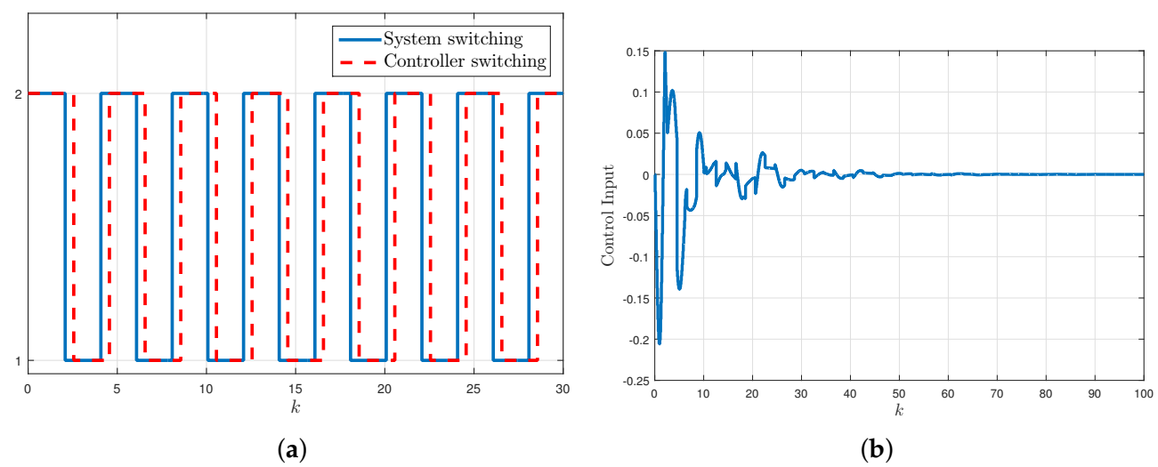
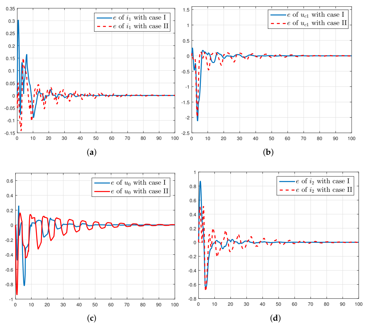
5. Numerical Examples

Example 1.

Consider a switched singular delayed system with two modes and the following parameters:

$$\begin{array}{cc}& \begin{array}{cc}& E=\left[\begin{array}{cc}3& 0\\ 1& 0\end{array}\right],A_1=\left[\begin{array}{cc}1.2& -0.3\\ 1.2& 1.38\end{array}\right],A_2=\left[\begin{array}{cc}-0.5& -0.3\\ -1& -0.1\end{array}\right],A_{d1}=\left[\begin{array}{cc}0.1& -0.1\\ 0& 0.1\end{array}\right],\hfill \\ & A_{d2}=\left[\begin{array}{cc}0.1& 0\\ 0.01& 0.1\end{array}\right],B_{11}=\left[\begin{array}{cc}-2& -1\\ -1& 0\end{array}\right],B_{12}=\left[\begin{array}{cc}-1.9& -1\\ -1& 1.3\end{array}\right],C_1=\left[\begin{array}{cc}0.5& -1.2\end{array}\right],\hfill \\ & C_2=\left[\begin{array}{cc}0.6& -1.1\end{array}\right],B_{21}=\left[\begin{array}{c}0.2\\ 0.1\end{array}\right],B_{22}=\left[\begin{array}{c}25\\ 10\end{array}\right],C_{21}=\left[\begin{array}{cc}0.001& 0\end{array}\right],C_{22}=\left[\begin{array}{cc}0.0001& 0\end{array}\right],\hfill \\ & D_1=0.6,D_2=0.7.\hfill \end{array}\hfill \end{array}$$

Since $deg\left(det(zE-A_2)\right)=deg(-0.25)=0<rank\left(E\right)=1$, pair $(E,A_2)$ is non causal. In this case, the unforced part of the considered subsystem is not admissible.

Let $d_m=2$, $d_M=3$, ${\lambda }_1=0.0001$, ${\lambda }_2=-0.0004$, ${\lambda }_3=-0.0002$, $K_{c1}=\left[\begin{array}{cc}-0.9& -0.01\\ -1& -3\end{array}\right]$, $K_{c2}=\left[\begin{array}{cc}-0.1& -1\\ -0.1& -1\end{array}\right]$; and take the ADT parameters $\alpha =0.6$, $\beta =1.03$, ${\mu }_1=1.2$, and ${\mu }_2=1.5$. Solving LMI conditions in Theorem 3, we get the minimum allowed ${\gamma }_m=0.6392$ and the following controller gains:

$$\begin{array}{c}\hfill \begin{array}{cc}\hfill K_1& =\left[\begin{array}{cc}-0.6334& -0.0375\\ -0.9743& -0.3784\end{array}\right],K_2=\left[\begin{array}{cc}-0.1141& -0.1352\\ -0.1413& -0.1637\end{array}\right]\hfill \\ \hfill L_1& =\left[\begin{array}{c}0.1394\\ -0.9710\end{array}\right],L_2=\left[\begin{array}{c}0.2519\\ -0.5930\end{array}\right]\hfill \end{array}\end{array}$$

(75)

For simulation purposes, the nonlinear function and the exogenous disturbance are given, respectively, as follows:

$$\begin{array}{cc}\hfill \phi \left(\varrho \right)& =2(M_2+M_1)\varrho +3(M_2-M_1)tan\left(\varrho \right).\hfill \\ \hfill w\left(k\right)& =sin\left(2k\right)e^{-0.9k}.\hfill \end{array}$$

where $M_1=0.1$ and $M_2=0.4$.

Under the variation of $d\left(k\right)$ depicted in Figure 4 and the switching signals depicted in Figure 2 with ${\Delta }_m=0.7$ and ${\tau }_a=2.1>{\tau }_a^{\ast }=1.8912$ by respecting the relationship in (59), simulation results are shown in Figure 3, Figure 4 and Figure 5, with initial conditions $x\left(0\right)={[670-700]}^T$ and $\widehat{x}\left(0\right)={\left[00\right]}^T$.

In the plotted Figure 3a–c, it can be seen that the system is stabilized regardless of time-varying delay, external disturbance, and sensor saturation. Moreover, for a non-causal system, a control problem is soved when the system states are unmeasured via the proposed control scheme, which is pertinent for the analysis in this paper.

From Figure 5, we can see that the evolution of the ratio ${\left|\right|z\left|\right|}_2/{\left|\right|w\left|\right|}_2$ under zero-initial condition tends to a constant value with a square root of about $0.6055$ which reveals that the $H_{\infty }$ disturbance attenuation level is less than the required minimum allowed value ${\gamma }_m=0.6392$ of γ.

Example 2.

To verify the merit of the controller strategy, the example of single-ended primary inductor converter (SEPIC) (Figure 6) presented in [46] is considered.

The parameters of the converter are illustrated in

Table 1. Converter parameters.

Acronyms	Definitions	Values/Units
$l_{c1}$	Input inductor	$1\times {10}^{-3}H$
$l_{c2}$	Output inductor	$0.5\times {10}^{-3}H$
$C_1$	Input capacitor	$0.1\times {10}^{-3}F$
$C_2$	Output capacitor	$0.1\times {10}^{-3}F$
$R_1$	Resistor of input inductor	$2\Omega$
$R_2$	Resistor of output inductor	$0.2\Omega$
R	Load resistor	$2\Omega$

.

The state variables of the system are the inductive currents $i_1$ and $i_2$, the capacitor voltage $u_{c1}$, and the output voltage $u_0$. The SEPIC scan be described by the following differential equations:

• When V is switched on:

  $$\begin{array}{cc}& \left\{\begin{array}{cc}\hfill {\dot{i}}_1& =-\frac{R_1}{l_{c1}}{i}_1+\frac{1}{l_{c1}}{E}_0\hfill \\ \hfill {\dot{u}}_{c1}& =-\frac{1}{C_1}{i}_2\hfill \\ \hfill {\dot{u}}_0& =-\frac{1}{R{C}_2}{u}_0\hfill \\ \hfill {\dot{i}}_2& =-\frac{R_2}{l_{c2}}{i}_2+\frac{1}{l_{c2}}{u}_{c1}\hfill \end{array}\right.\hfill \end{array}$$

  (76)
• When V is switched off:

  $$\begin{array}{cc}& \left\{\begin{array}{cc}\hfill {\dot{i}}_1& =-\frac{R_1}{l_{c1}}{i}_1-\frac{1}{l_{c1}}{u}_{c1}-\frac{1}{l_{c1}}{u}_0+\frac{1}{l_{c1}}{E}_0\hfill \\ \hfill {\dot{u}}_{c1}& =\frac{1}{C_1}{i}_1\hfill \\ \hfill {\dot{u}}_0& =\frac{1}{C_2}{i}_1+\frac{1}{C_2}{i}_2-\frac{1}{R{C}_2}{u}_0\hfill \\ \hfill {\dot{i}}_2& =-\frac{R_2}{l_{c2}}{i}_2-\frac{1}{l_{c2}}{u}_0\hfill \end{array}\right.\hfill \end{array}$$

  (77)

Set the control input $u\left(k\right)=E_0$ and the state vector as $x\left(k\right)={\left[i_1\left(k\right)u_{c1}\left(k\right)u_0\left(k\right)i_2\left(k\right)\right]}^T$.

We created the model (1) with the following data:

$$\begin{array}{cc}& \begin{array}{cc}& E=\left[\begin{array}{cccc}1& 0& 0& 0\\ 0& 1& 0& 0\\ 0& 0& 1& 0\\ 0& 0& 0& 1\end{array}\right],A_1=\left[\begin{array}{cccc}0.96& 0& 0& 0\\ 0& 1& 0& -0.2\\ 0& 0& 0.99& 0\\ 0& 0.04& 0& 0.992\end{array}\right],B_{11}=B_{12}=\left[\begin{array}{c}0.02\\ 0\\ 0\\ 0\end{array}\right],\hfill \\ & A_2=\left[\begin{array}{cccc}0.96& -0.02& -0.02& 0\\ 0.2& 1& 0& 0\\ 0.2& 0& 0.99& 0.2\\ 0& 0& -0.04& 0.992\end{array}\right],C_1=C_2=\left[\begin{array}{cccc}1& 0& 0& 0\\ 0& 1& 0& 0\\ 0& 0& 1& 0\end{array}\right],A_{d1}=A_{d2}=0,\hfill \\ & B_{21}=B_{22}=\left[\begin{array}{c}0.1\\ 0.1\\ 0.1\\ 0.1\end{array}\right],C_{21}=\left[\begin{array}{cccc}0.0001& 0.0001& 0& 0\end{array}\right],\hfill \end{array}\hfill \end{array}$$

(78)

$$\begin{array}{cc}& \begin{array}{cc}& C_{22}=\left[\begin{array}{cccc}0.0001& 0& 0.0001& 0\end{array}\right],D_1=0.1,D_2=0.01.\hfill \end{array}\hfill \end{array}$$

(79)

The nonlinear function and the exogenous disturbance are given as follows:

$$\begin{array}{cc}\hfill \phi \left(\varrho \right)& ={\displaystyle \frac{M_2+M_1}{2}}\varrho +{\displaystyle \frac{M_2-M_1}{2}}{\varrho }^2\hfill \\ \hfill \prime w\left(k\right)& =cos\left(2k\right)e^{-0.4k}.\hfill \end{array}$$

where $M_1=0.2$ and $M_2=0.5$.

case I: 

The method in this paper: Let ${\lambda }_1=-2$, ${\lambda }_2=-8$, ${\lambda }_3=-8$, $K_{c1}=[0.450.28-0.50]$, $K_{c2}=\left[0.4510.80\right]$, and ${\Delta }_m=0.5$; and ADT parameters ${\alpha }_1=0.3$, $\beta =1.03$, ${\mu }_1=1.2$, and ${\mu }_2=3$; a feasible result was obtained by Theorem 3 with the minimum allowed ${\gamma }_m=0.936$ and the following observer and controller gains:

$$\begin{array}{cc}\hfill & \begin{array}{cc}\hfill K_1& = \left[\begin{array}{cccc}0.0112& 0.0088& -0.0123& -0.0001\end{array}\right],\hfill \\ \hfill K_2& = \left[\begin{array}{cccc}-0.0321& -0.0186& -0.0337& 0.0007\end{array}\right],\hfill \\ \hfill L_1& =\left[\begin{array}{ccc}0.3826& -0.0202& 0.016\\ -0.0294& 0.4176& 0.0243\\ 0.0046& 0.017& 0.476\\ -0.0005& 0.0114& 0.0172\end{array}\right],L_2=\left[\begin{array}{ccc}0.1364& -0.002& -0.0307\\ 0.1179& 0.2011& -0.0052\\ 0.0830& 0.0227& 0.1435\\ 0.0025& -0.0051& -0.0151\end{array}\right].\hfill \end{array}\hfill \end{array}$$

(80)

case II: 

The method in [47]: The observer and controller gains were:

$$\begin{array}{cc}\hfill & \begin{array}{cc}\hfill K_1& = \left[\begin{array}{cccc}-19.0129& -3.7921& -3.3107& -7.1217\end{array}\right],\hfill \\ \hfill K_2& = \left[\begin{array}{cccc}-14.5563& -0.9161& -0.3893& -6.6751\end{array}\right],\hfill \\ \hfill L_1& =\left[\begin{array}{ccc}0.4081& 0.1669& 0.0882\\ 0.4601& 1.0845& -0.0181\\ 0.2778& -0.0630& 0.7716\\ -0.3815& -0.7171& -0.0399\end{array}\right],L_2=\left[\begin{array}{ccc}0.4448& -0.0478& 0.0512\\ 0.1588& 0.9432& 0.1189\\ -0.1689& -0.0161& 0.4380\\ -0.3458& -0.3748& 0.1141\end{array}\right].\hfill \end{array}\hfill \end{array}$$

(81)

Given the initial conditions $x\left(0\right)=\widehat{x}\left(0\right)={[1-120.1]}^T$, the simulation results are depicted in Figure 7 and Figure 8. The evolutions of the system states are shown in Figure 8. Figure 7 shows the evolution of the control input and the switching rule of the controller and the system in case I.

The results took into account that the converter system under asynchronous switching was stabilized even in the presence of the simultaneous sensor nonlinearity and exogenous disturbance.

Moreover, the control strategy guarantees the convergence of the system state when it is incompletely available for measurement.

To demonstrate the effectiveness of the proposed method in this work, we considered the resulting closed loop system performing by case II in Figure 9.

From Figure 9, it can be observed that all the presented controllers in case I and case II guarantee the convergence of the system. However, the evolutions of the estimated states were improved using the proposed gains in case I.

To further prove the merits of the proposed strategy, two quality criteria were considered to evaluate the states errors $e\left(k\right)=x\left(k\right)-\widehat{x}\left(k\right)$: integral squared error (ISE) and integral absolute error (IAE). The comparison is provided in

Table 2. Comparison of $e\left(k\right)$ for $k\in [0,100]$.

	ISE	IAE
Expression	${\sum }_{k=0}^{100}{\left(e\left(k\right)\right)}^2$	${\sum }_{k=0}^{100}\left|e\left(k\right)\right|$
case I	16	0.27
case II	19	0.39

.

From the results in Table 2, we deduced that the total deviation of e(k) was smaller for the method developed in this paper.

6. Conclusions

This work was a contribution to some issues in the control of switched singular non-linear time-varying systems with sensor saturation. An observer was considered to reconstruct the unmeasured system states with measurable outputs and an asynchronous control law was synthesized. Based on an appropriate Lyapunov–Krasovskii functional with a triple sum term and the ADT approach, delay-dependent sufficient conditions were proposed to ensure robust admissible of the closed loop system with $H_{\infty }$ performance. The resolvability of the corresponding observer-based controller conditions has also been established using the LMI technique. The merits of the presented results were verified through two examples.

As future work, it would be interesting to extend the results for the discrete-time stochastic Markov-jump singular systems and validate the obtained results on a photovoltaic practical platform.

References

1. Lin, J.; Fei, S.; Shen, J. Robust stability and stabilization for uncertain discrete-time switched singular systems with time-varying delays. J. Syst. Eng. Electron. 2010, 21, 650–657. [Google Scholar] [CrossRef]
2. Xu, Y.; Zhu, S.; Ma, S.; Han, Q.L. Finite-time stability and stabilization for a class of nonlinear discrete-time descriptor switched systems with time-varying delay. In Proceedings of the 33rd Chinese Control Conference (CCC), Nanjing, China, 28–30 July 2014; pp. 6025–6030. [Google Scholar]
3. Lin, J.; Fei, S.; Gao, Z. Control discrete-time switched singular systems with state delays under asynchronous switching. Int. J. Syst. Sci. 2013, 44, 1089–1101. [Google Scholar] [CrossRef]
4. Lin, J.; Fei, S.; Wu, Q. Reliable H filtering for discrete-time switched singular systems with time-varying delay. Circuits Syst. Signal Process. 2012, 31, 1191–1214. [Google Scholar] [CrossRef]
5. Zamani, I.; Shafiee, M. Stability analysis of uncertain switched singular time-delay systems with discrete and distributed delays. Optim. Control Appl. Methods 2015, 36, 1–28. [Google Scholar] [CrossRef]
6. Zhang, L.; Zhao, J.; Qi, X.; Li, F. Exponential stability for discrete-time singular switched time-delay systems with average dwell time. In Proceedings of the Control Conference (CCC), 2011 30th Chinese, Yantai, China, 22–24 July 2011; pp. 1789–1794. [Google Scholar]
7. Lin, J.; Fei, S.; Gao, Z.; Ding, J. Fault detection for discrete-time switched singular time-delay systems: An average dwell time approach. Int. J. Adapt. Control Signal Process. 2013, 27, 582–609. [Google Scholar] [CrossRef]
8. Li, S.; Xiang, Z. Stability, l1-gain and l-gain analysis for discrete-time positive switched singular delayed systems. Appl. Math. Comput. 2016, 275, 95–106. [Google Scholar] [CrossRef]
9. Ma, Y.; Fu, L. Finite-time H control for discrete-time switched singular time-delay systems subject to actuator saturation via static output feedback. Int. J. Syst. Sci. 2016, 47, 3394–3408. [Google Scholar] [CrossRef]
10. Kchaou, M.; Ahmadi, S.A. Robust Control for Nonlinear Uncertain Switched Descriptor Systems with Time Delay and Nonlinear Input: A Sliding Mode Approach. Complexity 2017, 2017, 14. [Google Scholar] [CrossRef] [Green Version]
11. Regaieg, M.; Kchaou, M.; Hajjaji, A.E.; Gassara, H.; Chaabane, M. Mode-dependent control design for discrete-time Switched Singular Systems with time varying delay. In Proceedings of the 2018 Annual American Control Conference, Milwaukee, WI, USA, 27–29 June 2018; pp. 374–379. [Google Scholar]
12. Lin, J.; Zhao, X.; Xiao, M.; Shen, J. Stabilization of discrete-time switched singular systems with state, output and switching delays. J. Frankl. Inst. 2019, 356, 2060–2089. [Google Scholar] [CrossRef]
13. Alexandra, M.; Paolo, M.; Andreas, Z. A multi input sliding mode control for Peltier Cells using a cold–hot sliding surface. J. Frankl. Inst. 2018, 355, 9351–9373. [Google Scholar] [CrossRef]
14. Regaieg, M.; Kchaou, M.; Hajjaji, A.E.; Chaabane, M. Robust H guaranteed cost control for discrete-time switched singular systems with time-varying delay. Optim. Control Appl. Methods 2019, 40, 119–140. [Google Scholar] [CrossRef]
15. Xing, M.; Xia, J.; Wang, J.; Meng, B.; Shen, H. Asynchronous H filtering for nonlinear persistent dwell-time switched singular systems with measurement quantization. Appl. Math. Comput. 2019, 362, 124578. [Google Scholar] [CrossRef]
16. Cheng, J.; Park, J.; Karimi, H.; Zhao, X. Static output feedback control of nonhomogeneous Markovian jump systems with asynchronous time delays. Inf. Sci. 2017, 399, 219–238. [Google Scholar] [CrossRef]
17. Zhao, X.; Tian, E.; Wang, L.; Li, H. Asynchronous control for discrete switched systems over network by using sojourn probability method. In Proceedings of the Control and Decision Conference (CCDC), 2016 Chinese, Yinchuan, China, 28–30 May 2016; pp. 962–967. [Google Scholar]
18. Wang, Y.E.; Zhao, J.; Jiang, B. Stabilization of a class of switched linear neutral systems under asynchronous switching. IEEE Trans. Autom. Control 2013, 58, 2114–2119. [Google Scholar] [CrossRef]
19. Xiang, Z.; Sun, Y.N.; Chen, Q. Stabilization for a class of switched neutral systems under asynchronous switching. Trans. Inst. Meas. Control 2012, 34, 793–801. [Google Scholar] [CrossRef]
20. Zhang, L.; Gao, H. Asynchronously switched control of switched linear systems with average dwell time. Automatica 2010, 46, 953–958. [Google Scholar] [CrossRef]
21. Zhao, X.; Shi, P.; Zhang, L. Asynchronously switched control of a class of slowly switched linear systems. Syst. Control Lett. 2012, 61, 1151–1156. [Google Scholar] [CrossRef]
22. Xiang, M.; Xiang, Z.; Karimi, H. Stabilization of positive switched systems with time-varying delays under asynchronous switching. Int. J. Control. Autom. Syst. 2014, 12, 939–947. [Google Scholar] [CrossRef] [Green Version]
23. Xiang, M.; Xiang, Z.; Karimi, H.R. Asynchronous L1 control of delayed switched positive systems with mode-dependent average dwell time. Inf. Sci. 2014, 278, 703–714. [Google Scholar] [CrossRef]
24. Regaieg, M.; Kchaou, M.; Bosche, J.; El-Hajjaji, A.; Chaabane, M. Asynchronous Output Feedback Control Design for Nonlinear Switched Singular Systems with Time Varying Delay. In Proceedings of the 2019 IEEE 58th Conference on Decision and Control (CDC), Nice, France, 11–13 December 2019; pp. 611–616. [Google Scholar]
25. Lin, J.; Fei, S.; Gao, Z. Stabilization of discrete-time switched singular time-delay systems under asynchronous switching. J. Frankl. Inst. 2012, 349, 1808–1827. [Google Scholar] [CrossRef]
26. Liu, L.L.; Wang, Y.E.; Wu, B.W. Asynchronous stabilization of switched singular systems with interval time varying delays. Int. J. Control Autom 2015, 8, 373–384. [Google Scholar] [CrossRef]
27. Lin, J.; Shi, Y.; Gao, Z.; Ding, J. Functional observer for switched discrete-time singular systems with time delays and unknown inputs. IET Control Theory Appl. 2015, 9, 2146–2156. [Google Scholar] [CrossRef]
28. Lin, J.; Gao, Z. Observers design for switched discrete-time singular time-delay systems with unknown inputs. Nonlinear Anal. Hybrid Syst. 2015, 18, 85–99. [Google Scholar] [CrossRef]
29. Han, Y.; Kao, Y.; Park, J. Robust nonfragile observer-based control of switched discrete singular systems with time-varying delays: A sliding mode control design. Int. J. Robust Nonlinear Control 2019, 29, 1462–1483. [Google Scholar] [CrossRef]
30. Sun, Y.; Ma, S. Observer-based asynchronous H control for a class of discrete time nonlinear switched singular systems. J. Frankl. Inst. 2020, 357, 5277–5301. [Google Scholar] [CrossRef]
31. Wang, T.; Tong, S. Observer-based output-feedback asynchronous control for switched fuzzy systems. IEEE Trans. Cybern. 2016, 47, 2579–2591. [Google Scholar] [CrossRef]
32. Zhang, M.; Shen, C.; Wu, Z.G. Asynchronous observer-based control for exponential stabilization of Markov jump systems. IEEE Trans. Circuits Syst. II Express Briefs 2019, 67, 2039–2043. [Google Scholar] [CrossRef]
33. Su, Y.; Zheng, C.; Mercorelli, P. Global finite-time stabilization of planar linear systems with actuator saturation. IEEE Trans. Circuits Syst. II Express Briefs 2016, 64, 947–951. [Google Scholar] [CrossRef]
34. Lian, J.; Li, C.; Liu, D. Input-to-state stability for discrete-time non-linear switched singular systems. IET Control Theory Appl. 2017, 11, 2893–2899. [Google Scholar] [CrossRef]
35. Liu, Y.; Wang, J.; Gao, C.; Tang, S.; Gao, Z. Input-to-state stability for a class of discrete-time nonlinear input-saturated switched descriptor systems with unstable subsystems. Neural Comput. Appl. 2018, 29, 417–424. [Google Scholar] [CrossRef]
36. Wang, J.; Ma, S.; Zhang, C. Finite-time stabilization for nonlinear discrete-time singular Markov jump systems with piecewise-constant transition probabilities subject to average dwell time. J. Frankl. Inst. 2017, 354, 2102–2124. [Google Scholar] [CrossRef]
37. Wei, Y.; Sun, L.; Jia, S.; Liu, K.; Meng, F. Disturbance attenuation and rejection for a class of switched nonlinear systems subject to input and sensor saturations. Math. Probl. Eng. 2019, 2019, 13. [Google Scholar] [CrossRef]
38. Cheng, J.; Zhan, Y. Nonstationary l2l filtering for Markov switching repeated scalar nonlinear systems with randomly occurring nonlinearities. Appl. Math. Comput. 2020, 365, 124714. [Google Scholar] [CrossRef]
39. Duan, R.; Li, J. Finite-time distributed H filtering for Takagi-Sugeno fuzzy system with uncertain probability sensor saturation under switching network topology: Non-PDC approach. Appl. Math. Comput. 2020, 371, 124961. [Google Scholar] [CrossRef]
40. Zhou, L.; Ho, D.W.; Zhai, G. Stability analysis of switched linear singular systems. Automatica 2013, 49, 1481–1487. [Google Scholar] [CrossRef]
41. Liu, Y.; Kao, Y.; Karimi, H.; Gao, Z. Input-to-state stability for discrete-time nonlinear switched singular systems. Inf. Sci. 2016, 358, 18–28. [Google Scholar] [CrossRef]
42. Wu, Z.G.; Shi, P.; Su, H.; Chu, J. Asynchronous l2 - l filtering for discrete-time stochastic Markov jump systems with randomly occurred sensor nonlinearities. Automatica 2014, 50, 180–186. [Google Scholar] [CrossRef]
43. Mathiyalagan, K.; Su, H.; Shi, P.; Sakthivel, R. Exponential H Filtering for Discrete-Time Switched Neural Networks With Random Delays. IEEE Trans. Cybern. 2015, 45, 676–687. [Google Scholar] [CrossRef]
44. Wang, G.; Xie, R.; Zhang, H.; Yu, G.; Dang, C. Robust Exponential H Filtering for Discrete-Time Switched Fuzzy Systems with Time-Varying Delay. Circuits Syst. Signal Process. 2016, 35, 117–138. [Google Scholar] [CrossRef]
45. Li, X.; Xiang, Z.; Karimi, H. Asynchronously switched control of discrete impulsive switched systems with time delays. Inf. Sci. 2013, 249, 132–142. [Google Scholar] [CrossRef]
46. Guo, S.; Zhu, F.; Jiang, B. Reduced-order switched UIO design for switched discrete-time descriptor systems. Nonlinear Anal. Hybrid Syst. 2018, 30, 240–255. [Google Scholar] [CrossRef]
47. Regaieg, M.; Kchaou, M.; Bosche, J.; El-Hajjaji, A.; Chaabane, M. Robust dissipative observer-based control design for discrete-time switched systems with time-varying delay. IET Control Theory Appl. 2019, 13, 3026–3039. [Google Scholar] [CrossRef]
Figure 1. Diagram of asynchronous switching.
Electronics 10 02334 g001
Figure 2. The system and controller switching signal.
Electronics 10 02334 g002
Figure 3. Simulation results for example 1. (a) Response and estimate trajectories of x 1 . (b) Input trajectory. (c) Response and estimate trajectories of x 2 .
Electronics 10 02334 g003
Figure 4. Variation of d ( k ) .
Electronics 10 02334 g004
Figure 5. Ratio evolution.
Electronics 10 02334 g005
Figure 6. Single-ended primary inductor converter.
Electronics 10 02334 g006
Figure 7. Switching signal and control input. (a) System and controller switching signal; (b) control input trajectory.
Electronics 10 02334 g007
Figure 8. Simulation results for example 2. (a) Response and estimate trajectories of i 1 . (b) Response and estimated trajectories of u c 1 . (c) Response and estimated trajectories of u 0 . (d) Response and estimate trajectories of i 2 .
Electronics 10 02334 g008
Figure 9. Estimation errors with case I and II. (a) Estimation error of i 1 . (b) Estimation error of u c 1 . (c) Estimation error of u 0 . (d) Estimation error of i 2 .
Electronics 10 02334 g009