Robust Control Optimization Based on Actuator Fault and Sensor Fault Compensation for Mini Motion Package Electro-Hydraulic Actuator

Abstract

In recent years, electro-hydraulic systems have been widely used in many industries and have attracted research attention because of their outstanding characteristics such as power, accuracy, efficiency, and ease of maintenance. However, such systems face serious problems caused simultaneously by disturbances, internal leakage fault, sensor fault, and dynamic uncertain equation components, which make the system unstable and unsafe. Therefore, in this paper, we focus on the estimation of system fault and uncertainties with the aid of advanced fault compensation techniques. First, we design a sliding mode observer using the Lyapunov algorithm to estimate actuator faults that produce not only internal leakage fault but also disturbances or unknown input uncertainties. These faults occur under the effect of payload variations and unknown friction nonlinearities. Second, Lyapunov analysis-based unknown input observer model is designed to estimate sensor faults arising from sensor noises and faults. Third, to minimize the estimated faults, a combination of actuator and sensor compensation fault is proposed, in which the compensation process is performed due to the difference between the output signal and its estimation. Finally, the numerical simulations are performed to demonstrate the effectiveness of the proposed method obtained under various faulty scenarios. The simulation results show that the efficiency of the proposed solution is better than the traditional PID controller and the sensor fault compensation method, despite the influence of noises.

1. Introduction

Nowadays, the breakthrough in information technology has promoted the progress of modern industry towards Industry 4.0. In meeting the requirements of precise control in industrial applications, electro-hydraulic actuator (EHA) systems play a significant role because they have the advantages of fast response, wide adjustment speed range, high power ratio, high speed, high accuracy, and high durability. Therefore, the EHA has been widely applied in industrial manufacture, agricultural machinery such as CNC machines, robotic manipulators, ships, and aerospace systems. However, EHA systems also have disadvantages including internal leakage, parametric uncertainties, external disturbance which makes these systems unstable, and the fluids inside them being often caustic and some seals [1,2,3,4]. To minimize the effect of parametric uncertainties in the EHA, nonlinear control schemes such as PID controller [5,6], adaptive control [7,8], Fuzzy-PID [9,10], sliding mode control [11,12,13,14,15], and neural network control [16,17,18,19] were proposed. The PID controller and adaptive control can reduce the adverse effect of parametric uncertainties, but they cannot completely deal with the influence of the above noises. Fuzzy-PID control depends highly on experience, which does not mention the system stability. Neural network control requires a large amount of training data and high computational complexity. Sliding mode control is applied to reduce uncertainty and turbulence but is effective only when the magnitude of the uncertainty and disturbance parameters is within the permissible limits and these disturbances and uncertainties in components can be considered as faults.

Hence, to ensure the stability of the EHA when operating and to prevent problems caused by faults of sensors and actuators, sensor fault detection and isolation (FDI) and fault accommodation are applied. These methods have become attractive topics, receiving considerable attention during the past two decades, to improve reliability and guarantee stability [20,21,22,23]. Reference [20] shows that fault detection and isolation filters are designed by applying residual filter synthesis algorithms to enable monitoring the sensor faults of electro-mechanical actuators to maintain possible adaptations in case of failures. In [21], the authors tried to improve small faults in the FDI method, using multiple residual generators. Here, the performance of FDI is characterized by the associated probability of detection and false alarm. In another approach, a novel fault diagnosis method based on quantum particle swarm optimization and least square support vector regression (LSSVR) algorithm to detect sensor faults for EHA has improved the prediction accuracy of the LSSVR model [22]. Further, to reduce the impact of faults, fault-tolerant control (FTC) algorithm is addressed [24,25,26,27,28]. In [24], Hongmei Liu et al. proposed an unscented Kalman Filter based fault diagnosis for hydraulic servo systems. The authors also examined two types of hydraulic servo system faults (i.e., abrupt fault in servo valve gain and slow wear fault in hydraulic cylinder piston) and conducted three different experiments to evaluate the outperformance of the suggested solution. To investigate the recent achievements in fault detection and isolation, and the pros and cons of various active FTC techniques, the authors conducted an in-depth review as presented in [25]. The authors in [26] presented tools of advanced fault-tolerant control systems to ensure fault detection efficiency and timely response, enhance fault recovery, prevent faults from propagating or developing into total failures, and reduce the risk of safety hazards. These methods describe a design of advanced fault-tolerant control systems for chemical processes that explicitly deal with actuator and controller failures, as well as sensor faults and data losses. A combination of diagnosis and fault-tolerant control is shown in [27], in which an EHA-based FTC model is proposed to track the system operation under unexpected sensor-fault conditions. Here, an unknown input observer (UIO) using the extended Kalman-Bucy algorithm is suggested in the combination with the robust sensor FDI model, system states estimator, and time-domain fault information. Once a fault occurs, the faulty sensor is replaced by the estimated output from the UIO to retain the system stability.

However, the FDI method and fault accommodation indicate only the alarm system failures. They make appropriate decisions to isolate the faults immediately to avoid heavy losses and dangerous situations that do not reduce the impacts of the faults. Thence, several actuator and sensor failure estimation algorithms have been developed. Actuator fault estimation is performed based on the UIO model, which is designed using the Lyapunov analysis and the linear matrix inequality (LMI) optimization algorithm to determine observer gain [28,29,30,31,32,33,34,35,36,37,38]. In [29], a UIO model is implemented utilizing Bayesian filter equations and estimates the states in two steps: time update and measurement update. In [30,31], the FTC scheme applied fault estimation (FE) to a system involving unknown input, uncertainty, bounded disturbance, and additive faults. Here, the FE and FTC schemes are integrated to ensure the stability of the closed-loop system affected by gain factors. In [32], the authors focused on the estimation of the sensor faults and the state variables, in which an induction machine-based UIO model was obtained from linear parameter varying (LPV) systems and the rotation speed was considered as a variable parameter. The Lyapunov theory is a promising solution to ensure the stability of the proposed approach. The observer efficiency is not only to investigate the presence of the current sensor faults but also to estimate sensor faults. It is done by calculating the observer gains based on the LMI technique. A sensor fault-tolerant control (SFTC) was developed to enhance the robust position tracking control capabilities of a class of electro-hydraulic actuators known as small motion packages (MMPs). This technique utilizes the PID controller to ensure the position response, then to obtain the desired results as shown in [33,34,35,36,37]. The gain parameters of the UIO model are achieved by solving the control error equations based on the LMI optimization algorithm; if the algorithm is feasible, the UIO system reaches asymptotic stability. A comparison between the PID control and the FTC error is provided to evaluate the performance of the controller failure. Actuator fault and sensor fault estimation are designed by augmented observers as shown in [38,39], and a scheme of sliding mode observer is also performed in [40,41,42,43]. In [40], Wenhan Zhang et al. developed an augmented descriptor to estimate the actuator faults via a robust fault estimation observer. In another approach, sliding mode observers for fault detection was investigated. Especially, some of the unique properties of sliding mode observer was thoroughly exploited in [41]. In [42], the authors developed an UIO-based augmented system which can estimate both sensor fault and system states. Also, to reduce actuator faults in linear multi-agent system, Shahram H. et al. [43] designed a distributed fault estimation model by applying sliding mode observer for each agent.

In this paper, a fault-tolerant control approach based on a robust fault estimator is carried out to reduce the impact of disturbance, actuator, and sensor fault, applied to electro-hydraulics actuator systems in the presence of simultaneous faults. Additionally, a fault estimator is designed by integrating the UIO model based on the LMI optimization algorithm and augmented system, such that the control error dynamic reaches the asymptotic state stability. Here, the FTC model acts as the fault signal compensation against impacts from actuator and sensor faults, as well as disturbance, and maintains the stability of the closed-loop system. The robustness of the actuator fault estimator using the sliding mode observer model for Lipschitz nonlinear EHA systems are presented. Further, a UIO model integrating the LMI optimization algorithm and augmenting system to estimate sensor fault and to determine residual are described for Lipschitz nonlinear EHA systems. The contributions of this work include:

(1)

Concurrent fault/state estimation techniques robust to partially unknown inputs are developed under the support of the input-stable theory.

(2)

A combination of fault compensation for fault-tolerant control model and PID controller creates a robust fault estimation that makes tolerant strategies simple to apply and to improve the control performance under the impact of faults and external disturbances.

(3)

Input-to-state stability theory based on LMI optimization algorithm and augmented system is addressed by the tolerant closed-loop control system. The error dynamics reach the asymptotic stable state, which is shown as an effective tool for handling fault control issues.

(4)

The proposed method is compared to the PID controller to evaluate the effectiveness and performance of the proposed solution.

The remainder of this paper is organized as follows: Section 2 introduces the overview of the mini motion package EHA model. Section 3 and Section 4 respectively present the robust actuator fault estimation and unknown input observers for nonlinear system. Our proposed solution, namely actuator-sensor fault tolerant control, is described in detail in Section 5. The simulation results and conclusion are shown in Section 6 and Section 7.

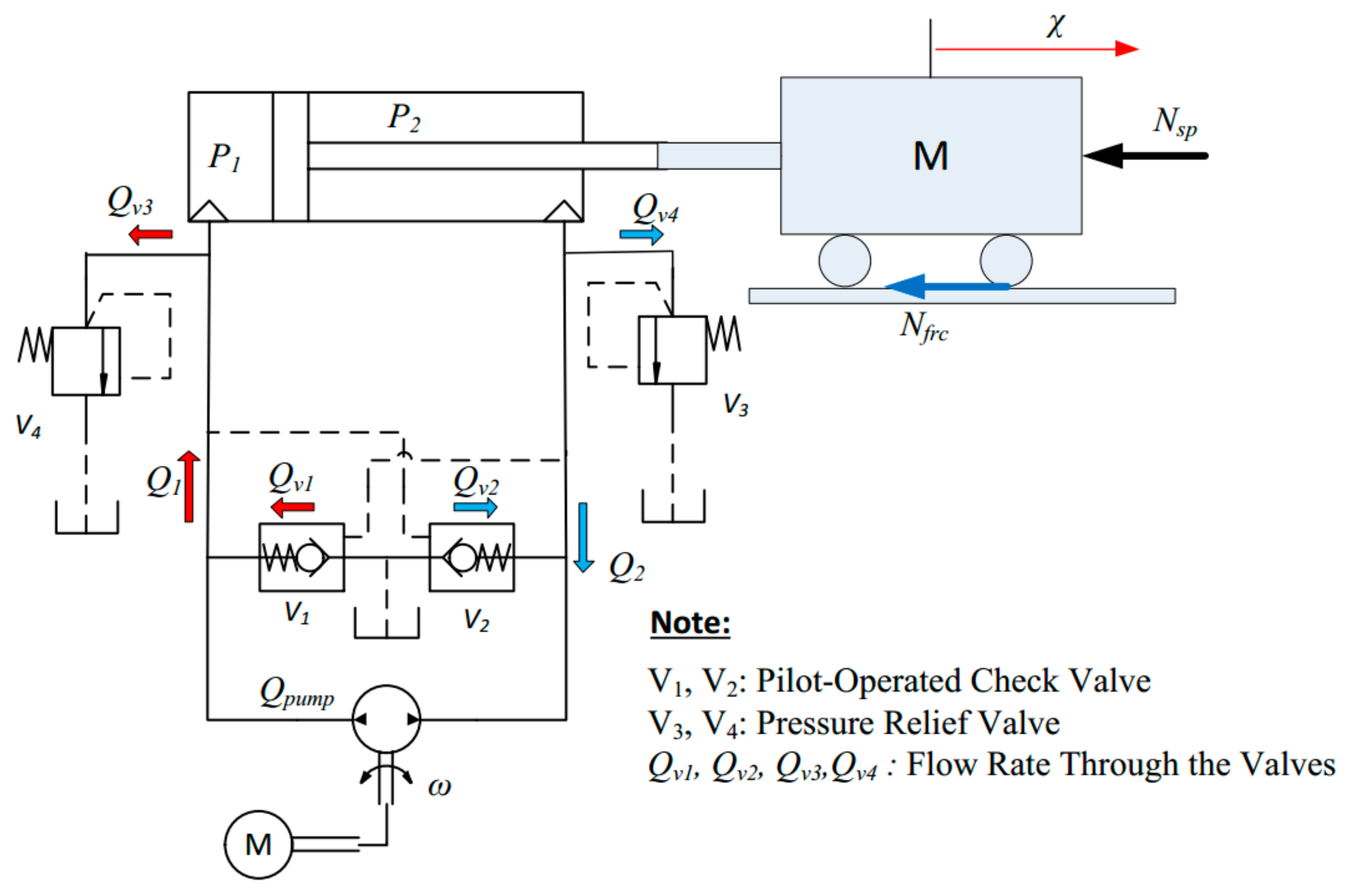
2. Modelling Mini Motion Package Electro-Hydraulics Actuator

Modelling of the EHA system is shown in Figure 1. The dynamics of the object M_p can be written as [15]:

$$M_p\ddot{\chi }+B_v\dot{\chi }+N_{sp}+N_{fr}+\zeta =S_1{P}_1-S_2{P}_2$$

(1)

where $M_p$ is the equivalent mass of the piston and object M, $\chi ,\hspace{0.17em}\dot{\chi }$, and $\ddot{\chi }$ are the position, acceleration, and the velocity of the piston, respectively, $S_1$, and $S_2$ are the areas in two chambers, respectively, $N_{sp}$ is the external load force of the spring of the piston, P₁ and P₂ are the pressures in two chambers, respectively, $B_v,\hspace{0.17em}{N}_{frc}$, and $\zeta$ are the viscosity damping coefficient, friction force, and unknown disturbance, respectively.

The spring force $N_{sp}$ can be computed as:

$$N_{sp}=K_{sp}\chi$$

(2)

where $K_{sp}$ is the stiffness of the spring.

The $N_{frc}$ friction force can be presented as [33]:

$$N_{frc}=\left\{\begin{array}{l}{\epsilon }_p\dot{\chi }+sign\left(\dot{\chi }\right)\left[N_{pc}+N_{ps}{e}^{-\left(\frac{\dot{\chi }}{v_{ps}}\right)}\right]\hspace{0.17em}\hspace{0.17em}\hspace{0.17em}\hspace{0.17em}\hspace{0.17em}\hspace{0.17em}\hspace{0.17em}\hspace{0.17em}\hspace{0.17em}\hspace{0.17em}\hspace{0.17em}\hspace{0.17em}\hspace{0.17em}\hspace{0.17em}\hspace{0.17em}\hspace{0.17em}\mathrm{with}\hspace{0.17em}\forall \dot{\chi }\ge 0\hspace{0.17em}\\ {\epsilon }_n\dot{\chi }+sign\left(\dot{\chi }\right)\left[N_{nc}+N_{ns}{e}^{-\left(\frac{\dot{\chi }}{v_{ns}}\right)}\right]\hspace{0.17em}\hspace{0.17em}\hspace{0.17em}\hspace{0.17em}\hspace{0.17em}\hspace{0.17em}\hspace{0.17em}\hspace{0.17em}\hspace{0.17em}\hspace{0.17em}\hspace{0.17em}\hspace{0.17em}\hspace{0.17em}\hspace{0.17em}\hspace{0.17em}\mathrm{with}\hspace{0.17em}\forall \dot{\chi }<0\end{array}\right.$$

(3)

where $N_{ps}$, and $N_{ns}$ are the static friction forces, $N_{pc}$ and $N_{nc}$ are the Coulomb friction forces, ${\epsilon }_p$ and ${\epsilon }_n$ are the viscous friction parameters, $v_{ps}$, and $v_{ns}$ are known as Stribeck velocity parameters for the positive and negative velocity motion of the cylinder, respectively.

Based on [33], the mathematical model of the EHA system can be presented as:

$$\left[\begin{array}{c}{\dot{\chi }}_1\\ {\dot{\chi }}_2\\ {\dot{\chi }}_3\\ {\dot{\chi }}_4\end{array}\right]=\left[\begin{array}{c}{\chi }_2\\ \frac{1}{M_p}\left[\left(S_1{\chi }_3-S_2{\chi }_4\right)-B_v{\chi }_2-N_{frc}-K_{sp}{\chi }_1-\zeta \right]\\ \frac{{\beta }_e}{V_{01}+S_1{\chi }_1}\left(Q_{pump}+Q_{13i}-S_1{\chi }_2\right)\\ \frac{{\beta }_e}{V_{02}-S_2{\chi }_1}\left(-Q_{pump}+Q_{24i}+S_2{\chi }_2\right)\end{array}\right]$$

(4)

where

$$\begin{gathered} {\left[\begin{array}{cccc}{\chi }_1& {\chi }_2& {\chi }_3& {\chi }_4\end{array}\right]}^T={\left[\begin{array}{cccc}\chi & \dot{\chi }& P_1& P_2\end{array}\right]}^T \\ {Q}_{13i}=Q_{1v}-Q_{3v}-Q_i; Q_{24i}=Q_{2v}-Q_{4v}+Q_i \end{gathered}$$

Scalar ${\beta }_e$ is the effective bulk modulus in each chamber and $Q_i$ is the internal leakage flow rate of the cylinder; $V_{01}$, and $V_{02}$ are the initial total control volumes of the first and the second chamber respectively [4]. $Q_{1v}$, and $Q_{2v}$ are the flow rate through of the pilot operated check valve on the left, and on the right, respectively. Similarly, $Q_{3v}$, and $Q_{4v}$ are the flow rate through the pressure relief valve on the left, and on the right, respectively. $Q_{pump}$, and $\omega$ are the pump flow rate, and the speed of the servo pump as shown in Figure 1, respectively.

To simplify the control process, (4) can be divided into two parts. The first part is designed as a mathematical model of the EHA system and presented as:

$$\left[\begin{array}{c}{\dot{\chi }}_1\\ {\dot{\chi }}_2\end{array}\right]=\left[\begin{array}{c}{\chi }_2\\ \frac{1}{M_p}\left[\left(S_1{\chi }_3-S_2{\chi }_4\right)-B_v{\chi }_2-N_{frc}-K_{sp}{\chi }_1-\zeta \right]\end{array}\right]$$

(5)

The second part plays the role of an input of system (6) which is described as:

$${\chi }_3={\displaystyle \int \frac{{\beta }_e}{V_{01}+S_1{\chi }_1}\left({\Delta }_p\mu +Q_{13i}-S_1{\chi }_2\right)}$$

(6)

$${\chi }_4={\displaystyle \int \frac{{\beta }_e}{V_{02}-S_2{\chi }_1}\left(-{\Delta }_p\mu +Q_{24i}+S_2{\chi }_2\right)}$$

(7)

where µ is the input control signal and $\mu =\omega$; ${\Delta }_p$ is the displacement, of the servo pump.

The dynamics equation of the EHA system is established based on (5) in the following form:

$$\dot{\chi }=\mathsf{\Phi }\chi +\mathsf{\Theta }u+f\left(\chi ,t\right)+\mathsf{\Psi }\zeta$$

(8)

where

$$\begin{array}{c}\mathsf{\Phi }=\left[\begin{array}{cc}0& 1\\ {\alpha }_1& {\alpha }_2\end{array}\right];\hspace{0.17em}\mathsf{\Theta }=\left[\begin{array}{cc}0& 0\\ \frac{S_1}{M_p}& -\frac{S_2}{M_p}\end{array}\right];\hspace{0.17em}f\left(\chi ,t\right)=\left[\begin{array}{c}0\\ -\frac{N_{frc}}{M_p}\end{array}\right]\\ {\alpha }_1=-\frac{K_{sp}}{M_p};\hspace{0.17em}{\alpha }_2=-\frac{B_v}{M_p};\mathsf{\Psi }=\left[\begin{array}{c}0\\ -\frac{1}{M_p}\end{array}\right];u=\left[\begin{array}{c}{\chi }_3\\ {\chi }_4\end{array}\right]\end{array}$$

Based on the nonlinear dynamic equation of the EHA in (8), the observer design and fault estimation are developed in the next section.

3. Robust Actuator Fault Estimation for Nonlinear System

The EHA system can be considered in the form:

$$\left\{\begin{array}{l}\dot{\chi }=\mathsf{\Phi }\chi +\mathsf{\Theta }u+f\left(\chi ,t\right)+F{f}_a+\zeta \\ y=\mathsf{\Upsilon }\chi \end{array}\right.$$

(9)

where $\chi \in {ℝ}^n,\hspace{0.17em}y\in {ℝ}^p,\hspace{0.17em}{f}_a\in {ℝ}^f$ and $u\in {ℝ}^q$ represent the state, output, unknown actuator fault, and input vector, respectively $\mathsf{\Phi }\in {ℝ}^{n\times n},\hspace{0.17em}\mathsf{\Theta }\in {ℝ}^{n\times q},F\in {ℝ}^{n\times q}$, and $\mathsf{\Upsilon }\in {ℝ}^{p\times n}$ denote known constant matrices with suitable dimensions.

Based on [43], a coordinate transformation $z\mapsto T_{\mathsf{\Upsilon }}\chi$ related to the invertible matrix

$$T_{\mathsf{\Upsilon }}={\left[\begin{array}{cc}{N}_{\mathsf{\Upsilon }}^T& {\mathsf{\Upsilon }}_{\mathsf{\Upsilon }}^T\end{array}\right]}^T$$

(10)

where the columns of $N\in {ℝ}^{n\times (n-p)}$ span the null space of $\mathsf{\Upsilon }$. Using the change of coordinate $z\mapsto T_{\mathsf{\Upsilon }}\chi$, $z\mapsto T_{\mathsf{\Upsilon }}\chi$, the triple ($\mathsf{\Phi },\mathsf{\Theta },\mathsf{\Upsilon }$) with det $T_{\mathsf{\Upsilon }}\ne 0$ has the following form:

$$T_{\mathsf{\Upsilon }}\mathsf{\Phi }{T}_{\mathsf{\Upsilon }}^{-1}=\left[\begin{array}{cc}{\mathsf{\Phi }}_{11}& {\mathsf{\Phi }}_{12}\\ {\mathsf{\Phi }}_{21}& {\mathsf{\Phi }}_{22}\end{array}\right];\hspace{0.17em}{T}_{\mathsf{\Upsilon }}\mathsf{\Theta }=\left[\begin{array}{c}{\mathsf{\Theta }}_1\\ {\mathsf{\Theta }}_2\end{array}\right];\hspace{0.17em}\mathsf{\Upsilon }{T}_{\mathsf{\Upsilon }}^{-1}=\left[\begin{array}{cc}0& I_p\end{array}\right]$$

Assumption 1.

The matrix pair ($\mathsf{\Phi },\mathsf{\Upsilon }$) is detectable

According to the Assumption 1, there exists a matrix$L\in {ℝ}^{n\times p}$ such that$\mathsf{\Phi }-L\mathsf{\Upsilon }$is stable, and thus for any$Q>0$,the Lyapunov equation below has a unique solution when$Q>0,\hspace{0.17em}\hspace{0.17em}U>0$ [43]:

$${\left(\mathsf{\Phi }-L\mathsf{\Upsilon }\right)}^{T}U+U\left(\mathsf{\Phi }-L\mathsf{\Upsilon }\right)=-Q$$

(11)

With$U\in {ℝ}^{n\times n},Q\in {ℝ}^{n\times n}$, these matrices can be expressed as:

$$U=\left[\begin{array}{cc}{U}_{11}& U_{12}\\ U_{21}& U_{22}\end{array}\right],Q=\left[\begin{array}{cc}{Q}_{11}& Q_{12}\\ Q_{21}& Q_{22}\end{array}\right]$$

(12)

These satisfy the condition$U_{11}\in {ℝ}^{q\times q}>0\hspace{0.17em}$,$U_{22}\in {ℝ}^{p\times p}$,$Q_{11}\in {ℝ}^{q\times q}>0\hspace{0.17em}$,and$Q_{22}\in {ℝ}^{p\times p}$if$\hspace{0.17em}U>0$ and$Q>0$.

Suppose that the$F$ has the following structure:

$$F={\left[\begin{array}{cc}{F}_1^T& F_2^T\end{array}\right]}^T \mathrm{and} F^{T}U=F\mathsf{\Upsilon }$$

(13)

where$F_1\in {ℝ}^{q\times r}$, and$F_2\in {ℝ}^{p\times r}$.

Lemma 1.

[43] If U and$Q$ have been partitioned as in (12),then

• $F_1+U_1^{-1}{U}_2{F}_2=0$ if (13)is satisfied
• The matrix ${\mathsf{\Phi }}_{11}+U_1^{-1}{U}_2{\mathsf{\Phi }}_{22}$ is stable if (11) is satisfied.

Assumption 2.

The actuator fault vector $f_a$ and disturbance vector$\zeta$ satisfy the following constraint:

$$\left|f_a\right|\le {\delta }_a \left|\zeta \left(t\right)\right|\le {\delta }_d$$

(14)

where${\delta }_a$ and${\delta }_d$two known positive constants.

3.1. Sliding Mode Observer Design

The design of the sliding mode observer performs is based on a linear transformation construction of coordinates $z=T\chi$ [43] to impose a specific structure on the fault distribution matrix z. The transformation matrix T has the following form:

$$T=\left[\begin{array}{cc}{I}_{n-p}& U_{11}^{-1}{U}_{12}\\ 0& I_p\end{array}\right]=\left[\begin{array}{c}{T}_1\\ T_2\end{array}\right]$$

(15)

where

$$T_1=\left[\begin{array}{cc}{I}_{n-p}& U_{11}^{-1}{U}_{12}\end{array}\right], \mathrm{and} T_2=\left[\begin{array}{cc}0& I_p\end{array}\right]$$

Equation (9), can be transformed into the new coordinate z as:

$$\left\{\begin{array}{l}\dot{z}={\mathsf{\Phi }}_{z}z+{\mathsf{\Theta }}_{z}u+Tf\left(T^{-1}z,t\right)+F_z{f}_a+T\zeta \\ y={\mathsf{\Upsilon }}_{z}z\end{array}\right.$$

(16)

where

$$\begin{gathered} {\mathsf{\Phi }}_z=T\mathsf{\Phi }{T}_{}^{-1}=\left[\begin{array}{cc}{\overline{\mathsf{\Phi }}}_{11}& {\overline{\mathsf{\Phi }}}_{12}\\ {\overline{\mathsf{\Phi }}}_{21}& {\overline{\mathsf{\Phi }}}_{22}\end{array}\right];\hspace{0.17em}{\mathsf{\Theta }}_z=T\mathsf{\Theta }=\left[\begin{array}{c}{\overline{\mathsf{\Theta }}}_1\\ {\overline{\mathsf{\Theta }}}_2\end{array}\right];\hspace{0.17em} \\ {\mathsf{\Upsilon }}_z=\mathsf{\Upsilon }{T}_{}^{-1}=\left[\begin{array}{cc}0& I_p\end{array}\right];\hspace{0.17em}{F}_z=\left[\begin{array}{c}{F}_1+U_{11}^{-1}{U}_{12}{F}_2\\ F_2\end{array}\right]=\left[\begin{array}{c}0\\ F_2\end{array}\right] \end{gathered}$$

System (16), can be rewritten as:

$$\hspace{0.17em}\left\{\begin{array}{l}{\dot{z}}_1={\overline{\mathsf{\Phi }}}_{11}{z}_1+{\overline{\mathsf{\Phi }}}_{12}{z}_2+T_{1}f(T^{-1}z,t)+T_1\zeta \hspace{0.17em}\\ {\dot{z}}_2={\overline{\mathsf{\Phi }}}_{21}{z}_1+{\overline{\mathsf{\Phi }}}_{22}{z}_2+T_{2}f(T^{-1}z,t)+{\overline{\mathsf{\Theta }}}_{2}u\hspace{0.17em}\hspace{0.17em}+F_2{f}_a+T_2\zeta \\ \hspace{0.17em}y\hspace{0.17em}\hspace{0.17em}=z_2\end{array}\right.$$

(17)

where

$$z={\left[\begin{array}{cc}{z}_1^T& z_2^T\end{array}\right]}^T \mathrm{with} \mathrm{the} \mathrm{column} z_1^{}\in {ℝ}^{n-p} \mathrm{and} z_2^{}\in {ℝ}^p$$

Based on [16], the sliding mode observer is designed as:

$$\hspace{0.17em}\left\{\begin{array}{l}{\dot{\widehat{z}}}_1={\overline{\mathsf{\Phi }}}_{11}{\widehat{z}}_1+{\overline{\mathsf{\Phi }}}_{12}y+T_{1}f(T^{-1}\widehat{z},t)+{\overline{\mathsf{\Theta }}}_{1}u\hspace{0.17em}\hspace{0.17em}\\ {\dot{\widehat{z}}}_2={\overline{\mathsf{\Phi }}}_{21}{\widehat{z}}_1+{\overline{\mathsf{\Phi }}}_{22}{\widehat{z}}_2+T_{2}f(T^{-1}\widehat{z},t)+{\overline{\mathsf{\Theta }}}_{2}u\hspace{0.17em}\hspace{0.17em}+\left({\overline{\mathsf{\Phi }}}_{22}-{\overline{\mathsf{\Phi }}}_0\right)\left(y-\widehat{y}\right)+\upsilon \\ \hspace{0.17em}\widehat{y}={\widehat{z}}_2\end{array}\right.$$

(18)

where ${\widehat{z}}_1^{}$ and ${\widehat{z}}_2^{}$ are the estimates of $z_1^{}$ and $z_2^{}$, respectively; $\widehat{y}$ denotes the estimate of y ${\mathsf{\Phi }}_0\in {ℝ}^{p\times p}$ is a stable design matrix. The discontinuous vector $\upsilon$ is computed by [43] and is given as:

$$\upsilon =\left\{\begin{array}{l}0\hspace{0.17em}\hspace{0.17em}\hspace{0.17em}\hspace{0.17em}\hspace{0.17em}\hspace{0.17em}\hspace{0.17em}\hspace{0.17em}\hspace{0.17em}\hspace{0.17em}\hspace{0.17em}\hspace{0.17em}\hspace{0.17em}\hspace{0.17em}\hspace{0.17em}\hspace{0.17em}\hspace{0.17em}\hspace{0.17em} if\hspace{0.17em}\hspace{0.17em}\hspace{0.17em}y-\widehat{y}=0\\ k\frac{U_0\left(y-\widehat{y}\right)}{‖U_0\left[y-\widehat{y}\right]‖}\hspace{0.17em}\hspace{0.17em}\hspace{0.17em}\hspace{0.17em}\hspace{0.17em}\hspace{0.17em}\hspace{0.17em}if\hspace{0.17em}\hspace{0.17em}y-\widehat{y}\ne 0\hspace{0.17em}\hspace{0.17em}\end{array}\right.$$

(19)

where $U_0$ is a symmetric positive definite matrix and the positive constant $k=\left|F_2\right|\rho +\eta$, $\rho$ and $\eta$ are the positive constants. If the state estimation error is defined by $\xi =z-\widehat{z}={\left[\begin{array}{cc}{\xi }_1^T& {\xi }_2^T\end{array}\right]}^T$, with ${\xi }_1^{}=z_1-{\widehat{z}}_1$ and ${\xi }_2^{}=z_2-{\widehat{z}}_2$.

Assumption 3.

Item of nonlinear function$f\left(\chi ,t\right)$ in (9) is Lipschitz with relation to the state$\chi$ and$\widehat{\chi }$:

$$‖f\left(\chi ,t\right)-f\left(\widehat{\chi },t\right)‖\le \lambda ‖\chi -\widehat{\chi }‖$$

(20)

Or

$$‖\Delta f‖\le \lambda ‖T^{-1}\xi ‖$$

where$\Delta f=f\left(\chi ,t\right)-f\left(\widehat{\chi },t\right)=f\left(T^{-1}z,t\right)-f\left(T^{-1}\widehat{z},t\right)$

λ: the known Lipschitz constant

Note that $\widehat{z}=\left[\begin{array}{cc}{\widehat{z}}_1& \widehat{y}\end{array}\right]$. Therefore, we has:

$$‖T^{-1}z-T^{-1}\widehat{z}‖=‖T^{-1}\left[\begin{array}{c}{\xi }_1\\ 0\end{array}\right]‖=‖{\xi }_1‖$$

(21)

and

$$‖\Delta f‖\le \lambda ‖{\xi }_1‖$$

(22)

Then state error dynamic system can be described as

$${\dot{\xi }}_1={\overline{\mathsf{\Phi }}}_{11}{\xi }_1+T_1\Delta f+T_1\zeta$$

(23)

$${\dot{\xi }}_2={\overline{\mathsf{\Phi }}}_{21}{\xi }_1+{\overline{\mathsf{\Phi }}}_0{\xi }_2+F_2{f}_a+T_2\zeta +T_2\Delta f-\upsilon$$

(24)

Theorem 1.

For system (9) with Assumptions 1–3. If there exists matrices$U_{11}=U_{11}^T>0$ $U_{12}$,$U_0=U_0^T>0$,${\mathsf{\Phi }}_0$, and initial conditions$‖\xi ‖\le \mu ‖\zeta ‖$with positive constants$\mu$,${\alpha }_0$, and${\alpha }_1$such that:

$$U_{11}{F}_1+U_{12}{F}_2=0$$

(25)

$$\left[\begin{array}{ccccccc}{\phi }_{11}& *& *& *& *& *& *\\ U_0{\overline{\mathsf{\Phi }}}_{21}& {\phi }_{22}& *& *& *& *& *\\ G_2^T{Z}^T& 0& -\mu I_p& *& *& *& *\\ G_1^T{Z}^T& 0& 0& -{\alpha }_1{I}_{n-p}& *& *& *\\ G_2^T{Z}^T& 0& 0& 0& -{\alpha }_1{I}_p& *& *\\ G_1^T{Z}^T& 0& 0& 0& 0& -\mu I_{n-p}& *\\ 0& U_0^T& 0& 0& 0& 0& -{\alpha }_0{I}_p\end{array}\right]\le 0$$

(26)

where

$$\begin{array}{l}{\phi }_{11}={\overline{\mathsf{\Phi }}}_{11}^{T}Z{G}_1^{}+Z{G}_1^{}{\overline{\mathsf{\Phi }}}_{11}^{}+\left({\alpha }_1+{\alpha }_0\right){\lambda }^2{I}_{n-p}+I_{n-p}\\ {\phi }_{22}={\overline{\mathsf{\Phi }}}_0^T{U}_0+U_0{\overline{\mathsf{\Phi }}}_0^{}+I_n\\ \hspace{1em}\hspace{1em}\hspace{1em}\hspace{1em} U_{11}=Z{G}_1^{} \mathrm{and} U_{12}=Z{G}_2^{}\end{array}$$

with$G_1^{}=\left(I_n-F{F}^{+}\right)\left[\begin{array}{c}{I}_{n-p}\\ 0\end{array}\right]$,$G_2^{}=\left(I_n-F{F}^{+}\right)\left[\begin{array}{c}0\\ I_p\end{array}\right]$and$F^{+}={\left(F^{T}F\right)}^{-1}{F}^T$then the observer error dynamic is asymptotically stable.

Proof of (25).

Based on Lemma 1 that if Assumption 2 is satisfied, then:

$$F_1+U_{11}^{-1}{U}_{12}{F}_2=0$$

(27)

(27) can be inferred from (25). □

Proof of (26).

Consider a Lyapunov function as:

$$V={\xi }^T{U}_z\xi$$

(28)

where

$$U_z=T^{-T}U{T}^{-1} \mathrm{and} \xi ={\left[\begin{array}{cc}{\xi }_1^T& {\xi }_2^T\end{array}\right]}^T$$

In the new coordinate, $U_z$ has the following quadratic as:

$$U_z=\left[\begin{array}{cc}{U}_{11}& 0\\ 0& U_0\end{array}\right] \mathrm{with} U_0=-U_{12}^T{U}_{11}^{-T}{U}_{12}+U_{22}$$

(29)

Concerning the time derivative (28), we have:

$$\begin{array}{l}\dot{V}={\dot{\xi }}_{}^T{U}_z\xi +{\xi }_{}^T{U}_z\dot{\xi }\\ \hspace{0.17em}\hspace{0.17em}\hspace{0.17em}\hspace{0.17em}\hspace{0.17em}={\dot{\xi }}_1^T{U}_{11}{\xi }_1+{\xi }_1^T{U}_{11}{\dot{\xi }}_1+{\dot{\xi }}_2^T{U}_0{\xi }_2+{\xi }_2^T{U}_0{\dot{\xi }}_2\\ \hspace{0.17em}\hspace{0.17em}\hspace{0.17em}\hspace{0.17em}\hspace{0.17em}={\dot{V}}_1+{\dot{V}}_2\end{array}$$

(30)

where

$$\begin{array}{l}{\dot{V}}_1={\dot{\xi }}_1^T{U}_{11}{\xi }_1+{\xi }_1^T{U}_{11}{\dot{\xi }}_1\\ \hspace{0.17em}\hspace{0.17em}\hspace{0.17em}\hspace{0.17em}\hspace{0.17em}={\xi }_1^T\left({\overline{\mathsf{\Phi }}}_{11}^T{U}_{11}+U_{11}{\overline{\mathsf{\Phi }}}_{11}^{}\right){\xi }_1+2{\xi }_1^T{U}_{11}{T}_1\Delta f_1+2{\xi }_1^T{U}_{11}{T}_1\zeta \end{array}$$

(31)

Since the inequality $2X^{T}Y\le \frac{1}{\alpha }{X}^{T}X+\alpha Y^{T}Y$ holds for any scalar α > 0 [43] then

$$\begin{array}{l}{\dot{V}}_1={\xi }_1^T\left({\overline{\mathsf{\Phi }}}_{11}^T{U}_{11}+U_{11}{\overline{\mathsf{\Phi }}}_{11}^{}\right){\xi }_1+2{\xi }_1^T{U}_{11}{T}_1\Delta f_1+2{\xi }_1^T{U}_{11}{T}_1\zeta \\ \hspace{0.17em}\hspace{0.17em}\hspace{0.17em}\hspace{0.17em}\hspace{0.17em}\le {\xi }_1^T\left({\overline{\mathsf{\Phi }}}_{11}^T{U}_{11}+U_{11}{\overline{\mathsf{\Phi }}}_{11}^{}+\frac{1}{{\alpha }_1}{U}_{11}{T}_1{T}_1^T{U}_{11}^T+{\alpha }_1{\lambda }^2{I}_{n-p}\right){\xi }_1+2{\xi }_1^T{U}_{11}{T}_1\zeta \end{array}$$

(32)

and

$$\begin{array}{ll}{\dot{V}}_2& ={\dot{\xi }}_2^T{U}_0{\xi }_2+{\xi }_2^T{U}_0{\dot{\xi }}_2\\ & ={\left[{\overline{\mathsf{\Phi }}}_{21}{\xi }_1+{\overline{\mathsf{\Phi }}}_0{\xi }_2+F_2{f}_a+T_2\zeta +T_2\Delta f-\upsilon \right]}^T{U}_0{\xi }_2\\ & \hspace{0.17em}\hspace{0.17em}\hspace{0.17em}+{\xi }_2^T{U}_0\left[{\overline{\mathsf{\Phi }}}_{21}{\xi }_1+{\overline{\mathsf{\Phi }}}_0{\xi }_2+F_2{f}_a+T_2\zeta +T_2\Delta f-\upsilon \right]\\ & ={\xi }_1^T{\overline{\mathsf{\Phi }}}_{21}^T{}_{21}{U}_0{\xi }_2+{\xi }_2^T{\overline{\mathsf{\Phi }}}_0^T{U}_0{\xi }_2+f_a^T{F}_2^T{U}_0{\xi }_2\hspace{0.17em}+{\zeta }^T{T}_2^T{U}_0{\xi }_2+\Delta f^T{T}_2^T{U}_0{\xi }_2-{\upsilon }^T{U}_0{\xi }_2\\ & \hspace{0.17em}\hspace{0.17em}\hspace{0.17em}+{\xi }_2^T{U}_0{\overline{\mathsf{\Phi }}}_{21}{\xi }_1+{\xi }_2^T{U}_0{\overline{\mathsf{\Phi }}}_0{\xi }_2+{\xi }_2^T{U}_0{F}_2{f}_a\hspace{0.17em}+{\xi }_2^T{U}_0{T}_2\zeta +{\xi }_2^T{U}_0{T}_2\Delta f-{\xi }_2^T{U}_0\upsilon \\ & ={\xi }_2^T\left({\overline{\mathsf{\Phi }}}_0^T{U}_0+U_0{\overline{\mathsf{\Phi }}}_0\right){\xi }_2+2{\xi }_2^T{U}_0{\overline{\mathsf{\Phi }}}_{21}{\xi }_1\hspace{0.17em}+2{\xi }_2^T{U}_0{F}_2{f}_a\hspace{0.17em}+2{\xi }_2^T{U}_0{T}_2\zeta +2{\xi }_2^T{U}_0{T}_2\Delta f\hspace{0.17em}-2{\xi }_2^T{U}_0\upsilon \\ & \le {\xi }_2^T\left({\overline{\mathsf{\Phi }}}_0^T{U}_0+U_0{\overline{\mathsf{\Phi }}}_0+\frac{1}{{\alpha }_2}{U}_0{T}_2{T}_2^T{U}_0^T\right){\xi }_2+2{\xi }_2^T{U}_0{\overline{\mathsf{\Phi }}}_{21}{\xi }_1\hspace{0.17em}+2{\xi }_2^T{U}_0{T}_2\zeta \hspace{0.17em}+{\alpha }_0{\lambda }^2{\xi }_1^T{\xi }_1^{}\hspace{0.17em}+2{\xi }_2^T{U}_0{F}_2{f}_a\end{array}$$

(33)

From (28) to (33); we have:

$$\begin{array}{ll}\dot{V}& \le {\xi }_1^T\left({\overline{\mathsf{\Phi }}}_{11}^T{U}_{11}+U_{11}{\overline{\mathsf{\Phi }}}_{11}+\frac{1}{{\alpha }_1}{U}_{11}{T}_1{T}_1^T{U}_{11}^T+{\alpha }_1{\lambda }^2{I}_{n-p}\right){\xi }_1\hspace{0.17em}\hspace{0.17em}+\hspace{0.17em}\hspace{0.17em}{\xi }_2^T\left({\overline{\mathsf{\Phi }}}_0^T{U}_0+U_0{\overline{\mathsf{\Phi }}}_0+\frac{1}{{\alpha }_2}{U}_0{T}_2{T}_2^T{U}_0^T\right){\xi }_2\\ & +2{\xi }_2^T{U}_0{\overline{\mathsf{\Phi }}}_{21}{\xi }_1+2{\xi }_2^T{U}_0{T}_2\zeta \hspace{0.17em}\hspace{0.17em}+{\alpha }_0{\lambda }^2{\xi }_1^T{\xi }_1^{}\hspace{0.17em}+2{\xi }_2^T{U}_0{F}_2{f}_a+2{\xi }_1^T{U}_{11}{T}_1\zeta \\ & ={\left[\begin{array}{c}{\xi }_1\\ {\xi }_2\\ \zeta \end{array}\right]}^T\left[\begin{array}{ccc}{\mathsf{\Omega }}_1& *& *\\ U_0{\overline{\mathsf{\Phi }}}_{21}& {\mathsf{\Omega }}_2& *\\ U_{11}^T+U_{12}& U_0^T& 0\end{array}\right]\left[\begin{array}{c}{\xi }_1\\ {\xi }_2\\ \zeta \end{array}\right]\\ & ={\left[\begin{array}{c}{\xi }_1\\ {\xi }_2\\ \zeta \end{array}\right]}^T{\mathsf{\Sigma }}_1\left[\begin{array}{c}{\xi }_1\\ {\xi }_2\\ \zeta \end{array}\right]\end{array}$$

(34)

where

$$\begin{array}{l}{\mathsf{\Omega }}_1={\overline{\mathsf{\Phi }}}_{11}^T{U}_{11}+U_{11}{\overline{\mathsf{\Phi }}}_{11}^{}+\frac{1}{{\alpha }_1}\left(U_{11}{U}_{11}^T+U_{12}{U}_{12}^T\right)+\left({\alpha }_1+{\alpha }_0\right){\lambda }^2{I}_{n-p}\\ {\mathsf{\Omega }}_2={\overline{\mathsf{\Phi }}}_0^T{U}_0+U_0{\overline{\mathsf{\Phi }}}_0^{}+\frac{1}{{\alpha }_2}{U}_0{U}_0^T\end{array}$$

and

$${\mathsf{\Sigma }}_1=\left[\begin{array}{ccc}{\mathsf{\Omega }}_1& *& *\\ U_0^{}{\overline{\mathsf{\Phi }}}_{21}& {\mathsf{\Omega }}_2& *\\ U_{11}^T+U_{12}& U_0^T& 0\end{array}\right]$$

To obtain the asymptotical stability of the state estimation errors ${\xi }_1$, and ${\xi }_2$ Equation (30) needs to satisfy the following condition: ${\dot{V}}_1\le 0$; ${\dot{V}}_2\le 0$.

Based on the initial condition $‖\xi ‖\le \mu ‖\zeta ‖$, the matrix J can be described as:

$$J={\left[\begin{array}{c}{\xi }_1\\ {\xi }_2\\ \zeta \end{array}\right]}^T\left[\begin{array}{ccc}{I}_{n-p}& *& *\\ 0& I_p& *\\ 0& 0& -\mu I_p\end{array}\right]\left[\begin{array}{c}{\xi }_1\\ {\xi }_2\\ \zeta \end{array}\right]\le 0$$

(35)

From (34) and (35), we can demonstrate:

$$\begin{array}{ll}{\mathsf{\Sigma }}_2& =\dot{V}+J\\ & ={\left[\begin{array}{c}{\xi }_1\\ {\xi }_2\\ \zeta \end{array}\right]}^T\left[\begin{array}{ccc}{\mathsf{\Omega }}_1+I_{n-p}& *& *\\ U_0{\overline{\mathsf{\Phi }}}_{21}& {\mathsf{\Omega }}_2+I_p& *\\ U_{11}^T+U_{12}& U_0^T& -\mu I_p\end{array}\right]\left[\begin{array}{c}{\xi }_1\\ {\xi }_2\\ \zeta \end{array}\right]\\ & ={\left[\begin{array}{c}{\xi }_1\\ {\xi }_2\\ \zeta \end{array}\right]}^T\mathsf{\Pi }\left[\begin{array}{c}{\xi }_1\\ {\xi }_2\\ \zeta \end{array}\right]\le 0\end{array}$$

(36)

where

$$\mathsf{\Pi }=\left[\begin{array}{ccc}{\mathsf{\Omega }}_1+I_{n-p}& *& *\\ U_0{\overline{\mathsf{\Phi }}}_{21}& {\mathsf{\Omega }}_2+I_p& *\\ U_{11}^T+U_{12}& U_0^T& -\mu I_p\end{array}\right]$$

The system obtains the asymptotical stability then $\mathsf{\Pi }$< 0 and apply Schur complement Lemma (36) for $\mathsf{\Pi }<0$, we obtain:

$$\begin{array}{ll}\mathsf{\Pi }& \le \left[\begin{array}{ccccccc}{\phi }_{11}& *& *& *& *& *& *\\ U_0{\overline{\mathsf{\Phi }}}_{21}& {\phi }_{11}& *& *& *& *& *\\ U_{12}^T& U_0^T& -\mu I_p& *& *& *& *\\ U_{11}^T& 0& 0& -{\alpha }_1{I}_{n-p}& *& *& *\\ U_{12}^T& 0& 0& 0& -{\alpha }_1{I}_p& *& *\\ U_{11}^T& 0& 0& 0& 0& -\mu I_{n-p}& *\\ 0& U_0^T& 0& 0& 0& 0& -{\alpha }_0{I}_p\end{array}\right]\\ & \le 0\end{array}$$

(37)

Substitution $U_{11}=Z{G}_1$ and $U_{12}=Z{G}_2$ into Equation (37), then (26) is satisfied.

Proof is complete.                 □

Moreover, Equation (25) needs to transform into a linear matrix inequality (LMI). This transformation is performed into the issue of finding the minimum of a positive scalar µ satisfying the following inequality constraint:

$$\left[\begin{array}{cc}\mu I_{n-p}& U_1{F}_1+U_2{F}_2\\ *& \mu I_r\end{array}\right]>0$$

(38)

By solving the LMI (26) and (38), terms $U_1,\hspace{0.17em}{U}_2,\hspace{0.17em}{U}_0$ and Q are obtained to calculate the observer gain ${\mathsf{\Phi }}_0=U_0^{-1}Q$ by substituting $\mathsf{\Upsilon }={\mathsf{\Upsilon }}_{z}T,\hspace{0.17em}R=T^{-1}{R}_z$ and $U=T^T{U}_{z}T$.

To compute the error dynamic system in (23) and (24), the sliding mode surface is defined as:

$$S=\left\{\left({\xi }_1,{\xi }_2\right)|{\xi }_2=0\right\}$$

(39)

Theorem 2.

Using the Assumptions 1–3, and the observer (18), the error systems (23) and (24) can begiven to the sliding surface (39)if gain τ is chosen for satisfaction:

$$\tau =‖{\overline{\mathsf{\Phi }}}_{21}‖\rho +‖F_2‖{\rho }_a+\varsigma +\lambda \psi +\gamma$$

(40)

where${\xi }_2\le \psi$,$\psi$ is the upper bound of$‖{\xi }_2‖$,$f_a\le {\rho }_a$with${\rho }_a$is a scalarand$‖{\xi }_1‖\le \rho$ with$\rho$ is a positive scalar.

Proof of (40).

Consider a Lyapunov function as:

$$V_a={\xi }_2^T{P}_0{\xi }_2$$

(41)

Derivative of $V_a$ in (41), we have:

$${\dot{V}}_a\hspace{0.17em}\hspace{0.17em}=\hspace{0.17em}\hspace{0.17em}{\xi }_2^T\left({\overline{\mathsf{\Phi }}}_0^T{U}_0+U_0{\overline{\mathsf{\Phi }}}_0\right){\xi }_2+2{\xi }_2^T{U}_0{\overline{\mathsf{\Phi }}}_{21}{\xi }_1+2{\xi }_2^T{U}_0{F}_2{f}_a\hspace{0.17em}+2{\xi }_2^T{U}_0{T}_2\zeta \hspace{0.17em}+2{\xi }_2^T{U}_0{T}_2\Delta f-2{\xi }_2^T{U}_0\upsilon$$

(42)

Based on (20), and since the matrix ${\mathsf{\Phi }}_0$ is the stable matrix. (42) is re-written as:

$$\begin{array}{ll}{\dot{V}}_a& \le 2{\xi }_2^T{U}_0{\overline{\mathsf{\Phi }}}_{21}{\xi }_1+2{\xi }_2^T{U}_0{F}_2{f}_a+2{\xi }_2^T{U}_0{T}_2\zeta \hspace{0.17em}+2{\xi }_2^T{U}_0{T}_2\Delta f-2{\xi }_2^T{U}_0\upsilon \hspace{0.17em}\\ & \le 2‖U_0{\xi }_2^{}‖‖{\overline{\mathsf{\Phi }}}_{21}‖‖{\xi }_1‖+2‖U_0{\xi }_2^{}‖‖F_2‖‖f_a‖+2‖U_0{\xi }_2^{}‖‖T_2‖‖\zeta ‖\hspace{0.17em}+2‖U_0{\xi }_2^{}‖‖T_2‖‖\Delta f‖-2\tau ‖U_0{\xi }_2^{}‖\\ & \le 2‖U_0{\xi }_2^{}‖\left(‖{\overline{\mathsf{\Phi }}}_{21}‖‖{\xi }_1‖+‖F_2‖{\rho }_a+‖T_2‖‖\zeta ‖\hspace{0.17em}+\lambda ‖{\xi }_2‖-\tau \right)\\ & =2‖U_0{\xi }_2^{}‖\left(‖{\overline{\mathsf{\Phi }}}_{21}‖\rho +‖F_2‖{\rho }_a+\varsigma \hspace{0.17em}+\lambda \psi -\tau \right)\end{array}$$

(43)

If the condition (40) holds, then with $\forall \gamma >0$, we have:

$${\dot{V}}_a\le -2\gamma ‖U_0{\xi }_2‖<0$$

(44)

                                 □

Therefore, the reachability condition is satisfied. Consequently, an ideal sliding motion will take place on the surface S in finite time [43].

3.2. Actuator Fault Estimation

The actuator fault estimation based on the proposed observer in the form of (19) is to estimate actuator faults using the so-called equivalent output injection [43]. Assuming that a sliding motion has been obtained, then ${\xi }_2=0$, and ${\dot{\xi }}_2=0$. Equation (24) is presented as:

$$0={\overline{\mathsf{\Phi }}}_{21}{\xi }_1+F_2{f}_a+T_2\Delta f+T_2\zeta -{\upsilon }_{eq}$$

(45)

where ${\upsilon }_{eq}$ is the named equivalent output error injection signal which is required to maintain the motion on the sliding surface [43].

The discontinuous component in (19) can be approximated by the continuous approximation as [43]:

$$\upsilon =\left\{\begin{array}{l}k\frac{U_0\left(y-\widehat{y}\right)}{‖U_0\left[y-\widehat{y}\right]‖+\delta }\hspace{0.17em}\hspace{0.17em}\hspace{0.17em}\hspace{0.17em}\hspace{0.17em}\hspace{0.17em}\hspace{0.17em}\hspace{0.17em}\hspace{0.17em}\hspace{0.17em}\hspace{0.17em}\hspace{0.17em}\hspace{0.17em}\hspace{0.17em}\hspace{0.17em}\xi \ne 0\\ 0\hspace{0.17em}\hspace{0.17em}\hspace{0.17em}\hspace{0.17em}\hspace{0.17em}\hspace{0.17em}\hspace{0.17em}\hspace{0.17em}\hspace{0.17em}\hspace{0.17em}\hspace{0.17em}\hspace{0.17em}\hspace{0.17em}\hspace{0.17em}\hspace{0.17em}\hspace{0.17em}\hspace{0.17em}\hspace{0.17em}\hspace{0.17em}\hspace{0.17em}\hspace{0.17em}\hspace{0.17em}\hspace{0.17em}\hspace{0.17em}\hspace{0.17em}\hspace{0.17em}\hspace{0.17em}\hspace{0.17em} otherwise\end{array}\right.\hspace{0.17em}\hspace{0.17em}\hspace{0.17em}\hspace{0.17em}\hspace{0.17em}\hspace{0.17em}$$

(46)

where δ is a small positive scalar to reduce the chattering effect, with this approximation, the error dynamics cannot slide on the surface S perfectly, but within a small boundary layer around it.

Based on [43], the actuator fault estimation is defined as:

$${\widehat{f}}_a=F_2^{+}{\upsilon }_{eq}$$

(47)

where

$$F_2^{+}={(F_2^T{F}_2)}^{-1}{F}_2^T$$

Equation (45) can be represented as:

$$f_a-{\widehat{f}}_a=-F_2^{+}{\overline{\mathsf{\Phi }}}_{21}{\xi }_1-F_2^{+}{T}_2\Delta f-F_2^{+}{T}_2\zeta$$

(48)

By considering the norm of (48), we obtain:

$$\begin{array}{ll}‖f_a-{\widehat{f}}_a‖& =‖F_2^{+}{\overline{\mathsf{\Phi }}}_{21}{\xi }_1+F_2^{+}{T}_2\Delta f-F_2^{+}{T}_2\zeta ‖\\ & \le {\sigma }_{\max }\left(F_2^{+}{\overline{\mathsf{\Phi }}}_{21}\right)‖{\xi }_1‖+{\sigma }_{\max }{F}_2^{+}\lambda ‖{\xi }_2‖+{\sigma }_{\max }{F}_2^{+}{T}_2‖\zeta ‖\\ & =\beta \xi +{\varsigma }_1‖\zeta ‖\end{array}$$

(49)

where

$$\beta =\left[\begin{array}{cc}{\sigma }_{\max }\left(F_2^{+}{\overline{\mathsf{\Phi }}}_{21}\right)& {\sigma }_{\max }\left(F_2^{+}\lambda \right)\end{array}\right], \mathrm{and} {\varsigma }_1={\sigma }_{\max }\left(F_2^{+}{T}_2\right)$$

Therefore, for a rather small $\beta \xi +{\varsigma }_1‖\zeta ‖$, then the actuator can be approximated as

$${\widehat{f}}_a=\tau \frac{F_2^{+}{U}_0\left[y-\widehat{y}\right]}{‖U_0\left[y-\widehat{y}\right]‖+\delta }$$

(50)

4. Unknown Inputs Observer (UIO) for Non-Linear Disturbance

In this section, an UIO method is designed to estimate the state vector for the computing arm of the residual in Section 5. We consider a nonlinear system in the following form:

$$\left\{\begin{array}{l}\dot{\chi }=\mathsf{\Phi }\chi +\mathsf{\Theta }u+f\left(\chi ,u\right)+\mathsf{\Psi }\zeta \\ y\hspace{0.17em}\hspace{0.17em}=\mathsf{\Upsilon }\chi +S{f}_s\end{array}\right.$$

(51)

where $x\in {ℝ}^n$, and $u\in {ℝ}^q$ are state vector and known inputs vector, respectively. $\xi \in {ℝ}^m$, and $y\in {ℝ}^p$ are unknown input disturbance vector and output vector of the system, respectively. $\mathsf{\Psi }$, and $S$ are known matrices with the suitable dimension, respectively.$f_s$ is the fault sensor.

Equation (51) can be rewritten as the following form:

$$\left\{\begin{array}{l}\overline{E}\dot{\overline{\chi }}=\overline{\mathsf{\Phi }}\overline{\chi }+\overline{\mathsf{\Theta }}u+\overline{f}\left(\chi ,u\hspace{0.17em}\right)+\overline{S}{f}_s+\overline{\mathsf{\Psi }}\zeta \\ \hspace{0.17em}\overline{y}=\overline{\mathsf{\Upsilon }}\overline{\chi }\end{array}\right.$$

(52)

where

$$\begin{gathered} \begin{array}{l}\overline{\mathsf{\Phi }}=\left[\begin{array}{cc}\mathsf{\Phi }& 0\\ 0& -I_s\end{array}\right];\overline{E}=\left[\begin{array}{cc}{I}_n& 0\\ 0& 0_s\end{array}\right];\overline{\mathsf{\Theta }}=\left[\begin{array}{c}\mathsf{\Theta }\\ 0\end{array}\right]\\ \overline{\mathsf{\Psi }}=\left[\begin{array}{c}\mathsf{\Psi }\\ 0\end{array}\right];\hspace{0.17em}\overline{f}\left(\chi ,u\hspace{0.17em}\right)=\left[\begin{array}{c}f\left(\chi ,u\hspace{0.17em}\right)\\ 0\end{array}\right]\end{array} \\ \overline{\mathsf{\Upsilon }}=\left[\begin{array}{cc}\mathsf{\Upsilon }& 1\end{array}\right];\overline{S}=\left[\begin{array}{c}0\\ I_s\end{array}\right];\overline{\chi }=\left[\begin{array}{c}\chi \\ f_s\end{array}\right]\in {ℝ}^{\overline{n}} \end{gathered}$$

The UIO model can be constructed in the influences of unknown inputs in the system (52) as:

$$\left\{\begin{array}{l}\dot{\overline{z}}=M\widehat{\overline{\chi }}+L\overline{y}-L\widehat{\overline{y}}+G\overline{f}\left(\widehat{\chi },u\hspace{0.17em}\right)+GNu\\ \widehat{\overline{\chi }}=\overline{z}+H\overline{y}\\ \widehat{\overline{y}}=\overline{\mathsf{\Upsilon }}\widehat{\overline{\chi }}\\ L=L_1+L_2\end{array}\right.$$

(53)

where $\widehat{\overline{x}}\in {ℝ}^{\overline{n}}$, and $\widehat{y}\in {ℝ}^p$ are state vector estimation of $\overline{x}$, and measurement output estimation vector, respectively. $\overline{z}\in {ℝ}^{\overline{n}}$ is the state vector of the observer. $M\in {ℝ}^{\overline{n}\times \overline{n}}$,$G\in {ℝ}^{\overline{n}\times \overline{n}}$, $H\in {ℝ}^{\overline{n}\times p}$, $L\in {ℝ}^{\overline{n}\times p}$, $L_1\in {ℝ}^{\overline{n}\times p}$, and $L_2\in {ℝ}^{\overline{n}\times p}$ are the observer matrices and these matrices should be designed according to the state estimation error vector.

The estimation error $\xi$ can be calculated as:

$$\begin{array}{ll}\overline{\xi }& =\overline{\chi }-\widehat{\overline{\chi }}\\ & =\overline{\chi }-\overline{z}-H\overline{y}\end{array}$$

(54)

and

$$\begin{array}{ll}\dot{\overline{\xi }}& =\dot{\overline{\chi }}-\dot{\widehat{\overline{\chi }}}\\ & =\dot{\overline{\chi }}-\dot{\overline{z}}-H\overline{\mathsf{\Upsilon }}\dot{\overline{\chi }}\\ & =\left(I_n-H\overline{\mathsf{\Upsilon }}\right)\dot{\overline{\chi }}-\dot{\overline{z}}\\ & =G\dot{\overline{\chi }}-\dot{\overline{z}}\end{array}$$

(55)

where

$$G=I_{\overline{n}}-H\overline{\mathsf{\Upsilon }}$$

(56)

The measurement error may be calculated as

$$\begin{array}{ll}{\overline{\xi }}_y^{}& =\overline{y}-\widehat{\overline{y}}\\ & =\overline{\mathsf{\Upsilon }}\overline{\xi }\end{array}$$

(57)

From (52), we have:

$$G\overline{E}\dot{\overline{\chi }}=G\overline{\mathsf{\Phi }}\overline{\chi }+G\overline{\mathsf{\Theta }}u+G\overline{f}\left(\chi ,u\right)+G\overline{S}\hspace{0.17em}{f}_s+G\overline{\mathsf{\Psi }}\zeta$$

(58)

From (58), we can write as:

$$\begin{array}{ll}\dot{\widehat{\overline{\chi }}}& =\dot{\overline{z}}+H\dot{\overline{y}}\\ & =M\widehat{\overline{\chi }}+L\overline{\mathsf{\Upsilon }}\overline{\chi }-L\overline{\mathsf{\Upsilon }}\widehat{\overline{\chi }}+G\overline{f}\left(\widehat{\chi },u\hspace{0.17em}\right)+GNu+H\overline{\mathsf{\Upsilon }}\dot{\overline{\chi }}\end{array}$$

(59)

By substituting (56) and (58) into (59), we have:

$$\begin{array}{l}G\overline{E}\dot{\overline{\chi }}-\dot{\widehat{\overline{\chi }}}\\ =G\overline{\mathsf{\Phi }}\overline{\chi }+G\overline{\mathsf{\Theta }}u+G\overline{f}\left(\chi ,u\right)+G\overline{S}\hspace{0.17em}{f}_s+G\overline{\mathsf{\Psi }}\zeta \hspace{0.17em}-M\widehat{\overline{\chi }}-L\overline{\mathsf{\Upsilon }}\overline{\chi }+L\overline{\mathsf{\Upsilon }}\widehat{\overline{\chi }}-G\overline{f}\left(\widehat{\chi },u\hspace{0.17em}\right)-GNu-H\overline{\mathsf{\Upsilon }}\dot{\overline{\chi }}\end{array}$$

(60)

The estimation error (61) can be reduced to

$$\dot{\overline{\xi }}=\left(G\overline{\mathsf{\Phi }}-L\overline{\mathsf{\Upsilon }}\right)\overline{\xi }+G\Delta \overline{f}+G\overline{S}\hspace{0.17em}{f}_s+G\overline{\mathsf{\Psi }}\zeta$$

(61)

where

$$\begin{array}{l}G\overline{E}+H\overline{\mathsf{\Upsilon }}=I_{\overline{n}}\\ M=G\overline{\mathsf{\Phi }}\\ \Delta \overline{f}=\overline{f}\left(\chi ,u\hspace{0.17em}\right)-\overline{f}\left(\widehat{\chi },u\hspace{0.17em}\right)\\ \overline{\mathsf{\Theta }}-N=0\end{array}$$

In which, matrix G is selected as:

$$G=\left[\begin{array}{cc}{I}_n& 0\\ -\overline{\mathsf{\Upsilon }}& 0\end{array}\right] \mathrm{and} H=\left[\begin{array}{cc}0& I_s\end{array}\right]$$

The matrix $H$ can be computed from (56) as following:

$$H=-\mathsf{\Psi }{(\mathsf{\Upsilon }\mathsf{\Psi })}^{†}$$

(62)

This matrix depends on the matrix rank $\mathsf{\Upsilon }\mathsf{\Psi }$, $H$ exists if $rank(\mathsf{\Upsilon }\mathsf{\Psi })=m$.

In general, based on [32,33,34,35,36,37], the matrix $H$ can be expressed as:

$$\begin{array}{ll}H& =\mathsf{\Psi }{\left(\mathsf{\Upsilon }\mathsf{\Psi }\right)}^{†}+Y\left(I-\left(\mathsf{\Upsilon }\mathsf{\Psi }\right){\left(\mathsf{\Upsilon }\mathsf{\Psi }\right)}^{†}\right)\\ & =U_s+Y{V}_s\end{array}$$

(63)

where

$$\hspace{0.17em}{U}_s=\mathsf{\Psi }{\left(\mathsf{\Upsilon }\mathsf{\Psi }\right)}^{†};\hspace{0.17em}{V}_s=I-\left(\mathsf{\Upsilon }\mathsf{\Psi }\right){\left(\mathsf{\Upsilon }\mathsf{\Psi }\right)}^{†}; \hspace{0.17em}{\left(\mathsf{\Upsilon }\mathsf{\Psi }\right)}^{†}={\left[{\left(\mathsf{\Upsilon }\mathsf{\Psi }\right)}^T\left(\mathsf{\Upsilon }\mathsf{\Psi }\right)\right]}^{-1}{\left(\mathsf{\Upsilon }\mathsf{\Psi }\right)}^T$$

To simplify calculating, (61) can be presented as:

$$G\mathsf{\Phi }-K\mathsf{\Upsilon }=M$$

(64)

where

$$K=MH+L$$

Gain $L$ can be inferred from (64) as

$$\begin{array}{ll}L& =K-\left(G\mathsf{\Phi }-K\mathsf{\Upsilon }\right)H\\ & =K\left(I+\mathsf{\Upsilon }H\right)-G\mathsf{\Phi }H\end{array}$$

(65)

The nonlinear component $\Delta \overline{f}$ of the nonlinear system satisfies the condition with Lipschitz constant δ_s, such as:

$$‖\Delta f‖\le {\delta }_s‖\chi -\widehat{\chi }‖$$

(66)

where

$$\Delta f=f\left(\chi ,u\hspace{0.17em}\right)-f\left(\widehat{\chi },u\hspace{0.17em}\right)$$

and

$$‖\Delta \overline{f}‖\le {\overline{\delta }}_s‖\overline{\chi }-\widehat{\overline{\chi }}‖$$

with

$${\overline{\delta }}_s=\left[\begin{array}{cc}{\delta }_s{I}_n& 0\\ 0& 0_s\end{array}\right]$$

Equation (66), we can infer as:

$${\mathsf{\Pi }}_s=\Delta {\overline{f}}^T\Delta \overline{f}-{\overline{\delta }}_s^T{\overline{\delta }}_s^{}{\overline{\xi }}^T\overline{\xi }\le 0$$

(67)

where

$$\hspace{0.17em}\hspace{0.17em}\hspace{0.17em}{\mathsf{\Pi }}_s={\left[\begin{array}{c}\overline{\xi }\\ \Delta \overline{f}\\ \zeta \\ f_s\end{array}\right]}^T\left[\begin{array}{cccc}-{\overline{\delta }}_s^T{\overline{\delta }}_s^T& *& *& *\\ 0& I_{\overline{n}}& *& *\\ 0& 0& 0& *\\ 0& 0& 0& 0\end{array}\right]\left[\begin{array}{c}\overline{\xi }\\ \Delta \overline{f}\\ \zeta \\ f_s\end{array}\right]\le 0$$

Lemma 2.

[41] The necessary and enough conditions for the existence of UIO in (54), if the system (52) guarantees as follows:

(a)

$rank(\mathsf{\Upsilon }\mathsf{\Psi })=rank(\mathsf{\Psi })$

(b)

$\left[\begin{array}{cc}\mathsf{\Phi }-I_n& \mathsf{\Psi }\\ \mathsf{\Upsilon }& 0\end{array}\right]=n+p$, and $\mathsf{\Psi }$ is a full column rank

(c)

$\left[\begin{array}{cc}\mathsf{\Phi }-z{I}_n& \mathsf{\Psi }\\ \mathsf{\Upsilon }& 0\end{array}\right]=n+p\hspace{0.17em}\hspace{0.17em}\hspace{0.17em}\hspace{0.17em}\forall z$with $\left|z\right|>1$

Lemma 3.

[33] For the equation in the following form

$$\dot{\iota }={\mathsf{\Phi }}_s\iota +{\mathsf{\Upsilon }}_{s}u$$

(68)

The eigenvalues of a given matrix ${\mathsf{\Phi }}_s\in {ℝ}^{n\times n}$belong to the circular region $D\left({\alpha }_s,{\rho }_s\right)$with the centerα_s + j0 and the radius ${\rho }_s$if and only if there exists a symmetric positive definite matrix $P\in {ℝ}^{n\times n}$such that the following condition holds

$$\left[\begin{array}{cc}-P& P\left({\mathsf{\Phi }}_s-{\alpha }_s{I}_n\right)\\ *& -{\rho }^{2}P\end{array}\right]<0$$

(69)

Theorem 3.

The system (52) exists a robust UIO in the form of (53) such that output the estimation error satisfies$‖{\xi }_y‖\le {\gamma }_s‖\zeta ‖$, and a prescribed circular region$D\left({\alpha }_s,{\rho }_s\right)$if there exists a positive-definite symmetric matrix$P\in {ℝ}^{n\times n}$, matrix$Q_s\in {ℝ}^{n\times p}$, and the positive scalars${\gamma }_s$, and${\phi }_s$such that the following inequalities (70) and (71) hold:

$$\left[\begin{array}{cccccc}{\theta }_{11}& PG& PG\overline{\mathsf{\Psi }}& PG\overline{S}& {\overline{\mathsf{\Upsilon }}}_{}^T& {\overline{\mathsf{\Upsilon }}}_{}^T\\ *& -{\phi }_s{I}_{\overline{n}}& 0& 0& 0& 0\\ *& *& -{\gamma }_s{I}_d& 0& 0& 0\\ *& *& *& -{\epsilon }_s{I}_s& 0& 0\\ *& *& *& *& -{\gamma }_s{I}_p& 0\\ *& *& *& *& *& -{\epsilon }_s{I}_p\end{array}\right]<0$$

(70)

$${\theta }_{11}={\left(G\overline{\mathsf{\Phi }}\right)}^{T}P+PG\overline{\mathsf{\Phi }}-{\overline{\mathsf{\Upsilon }}}^T{Q}_s^T-Q_s\overline{\mathsf{\Upsilon }}+{\phi }_s{\overline{\delta }}_{}^T\overline{\delta }$$

and

$$\left[\begin{array}{cc}-P& PG\overline{\mathsf{\Phi }}-Q_s\overline{\mathsf{\Upsilon }}-{\alpha }_{s}P\\ *& -{\rho }^{2}P\end{array}\right]<0$$

(71)

where

$$Q_s=PL$$

Proof of (70).

Consider a Lyapunov function as:

$$V={\overline{\xi }}^{T}P\overline{\xi }$$

(72)

Derivative the Equation (72), we have:

$$\begin{array}{ll}\dot{V}& ={\dot{\overline{\xi }}}^{T}P\overline{\xi }+{\overline{\xi }}^{T}P\dot{\overline{\xi }}\\ & ={\left[M\overline{\xi }+G\Delta \overline{f}+G\overline{\mathsf{\Psi }}\zeta +G\overline{S}\hspace{0.17em}{f}_s\right]}^{T}P\overline{\xi }\hspace{0.17em}\hspace{0.17em}+{\overline{\xi }}^{T}P\left[M\overline{\xi }+G\Delta \overline{f}+G\overline{\mathsf{\Psi }}\zeta +G\overline{S}\hspace{0.17em}{f}_s\right]\\ & ={\overline{\xi }}^T{M}^{T}P\overline{\xi }+\Delta {\overline{f}}^T{G}^{T}P\overline{\xi }+{\zeta }^T{\left(G\overline{\mathsf{\Psi }}\right)}^{T}P\overline{\xi }\hspace{0.17em}+f_s^T{(G\overline{S})}^{T}P\overline{\xi }+{\overline{\xi }}^{T}PM\overline{\xi }\\ & \hspace{0.17em}\hspace{0.17em}\hspace{0.17em}+{\overline{\xi }}^{T}PG\Delta \overline{f}+{\overline{\xi }}^{T}PG\overline{\mathsf{\Psi }}\zeta +{\overline{\xi }}^{T}PG\overline{S}{f}_s^{}\\ & ={\left[\begin{array}{c}\overline{\xi }\\ \Delta \overline{f}\\ \zeta \\ f_s\end{array}\right]}^T\left[\begin{array}{cccc}{M}^{T}P+PM& PG& PG\overline{\mathsf{\Psi }}& PG\overline{S}\\ *& 0& 0& 0\\ *& *& 0& 0\\ *& *& *& 0\end{array}\right]\left[\begin{array}{c}\overline{\xi }\\ \Delta \overline{f}\\ \zeta \\ f_s\end{array}\right]\end{array}$$

(73)

The steady state of the system is obtained if the (73) inequality ≤ 0 exists.

According to (67) and (73), a matrix $V_L$ can be archived if there exists a scalar ${\phi }_s$ > 0 that satisfy for the system stable condition as:

$$V_L=\dot{V}-{\phi }_s{\mathsf{\Pi }}_s$$

Or

$$V_L={\left[\begin{array}{c}\overline{\xi }\\ \Delta \overline{f}\\ \zeta \\ f_s\end{array}\right]}^T\left[\begin{array}{cccc}{M}^{T}P+PM& PG& PG\overline{\mathsf{\Psi }}& PG\overline{S}\\ *& 0& 0& 0\\ *& *& 0& 0\\ *& *& *& 0\end{array}\right]\left[\begin{array}{c}\overline{\xi }\\ \Delta \overline{f}\\ \zeta \\ f_s\end{array}\right]\hspace{0.17em}\hspace{0.17em}+{\left[\begin{array}{c}\overline{\xi }\\ \Delta \overline{f}\\ \zeta \\ f_s\end{array}\right]}^T\left[\begin{array}{cccc}{\phi }_s{\overline{\delta }}_{}^T\overline{\delta }& 0& 0& 0\\ *& -{\phi }_s{I}_{\overline{n}}& 0& 0\\ *& *& 0& 0\\ *& *& *& 0\end{array}\right]\left[\begin{array}{c}\overline{\xi }\\ \Delta \overline{f}\\ \zeta \\ f_s\end{array}\right]$$

$$\hspace{0.17em}{V}_L={\left[\begin{array}{c}\overline{\xi }\\ \Delta \overline{f}\\ \zeta \\ f_s\end{array}\right]}^T\left[\begin{array}{cccc}{\rho }_{11}& PG& PG\overline{\mathsf{\Psi }}& PG\overline{S}\\ *& -{\phi }_s{I}_{\overline{n}}& 0& 0\\ *& *& 0& 0\\ *& *& *& 0\end{array}\right]\left[\begin{array}{c}\overline{\xi }\\ \Delta \overline{f}\\ \zeta \\ f_s\end{array}\right]$$

(74)

where

$${\rho }_{11}=M^{T}P+PM+{\phi }_s{\overline{\delta }}_{}^T\overline{\delta }$$

In addition, based on the initial measurement error condition $‖{\xi }_y‖\le {\gamma }_s‖\zeta ‖$ of output, and $‖{\xi }_y‖\le {\epsilon }_s‖f_s‖$ with scalars ${\gamma }_s$ and ${\epsilon }_s$, then the matrix $J_s$ can be written as:

$$\begin{array}{ll}{J}_s& =\left(\frac{1}{{\gamma }_s}{\overline{\xi }}_y^T{\overline{\xi }}_y-{\gamma }_s{\zeta }^T\zeta \right)+\left(f_s^T{f}_s-{\epsilon }_s^2{I}_s\right)\\ & =\frac{1}{{\gamma }_s}{\overline{\xi }}^T{\overline{\mathsf{\Upsilon }}}^T\overline{\mathsf{\Upsilon }}\overline{\xi }-{\gamma }_s{\zeta }^T\zeta +\frac{1}{{\epsilon }_s}{\overline{\xi }}^T{\overline{\mathsf{\Upsilon }}}^T\overline{\mathsf{\Upsilon }}\overline{\xi }-{\epsilon }_s{f}_s^T{f}_s\\ & \le 0\end{array}$$

(75)

Or

$$J_s={\vartheta }^T\left[\begin{array}{cccc}\left(\frac{1}{{\gamma }_s}+\frac{1}{{\epsilon }_s}\right){\overline{\mathsf{\Upsilon }}}^T\overline{\mathsf{\Upsilon }}& *& *& *\\ 0& 0& *& *\\ 0& 0& -{\gamma }_s{I}_{\zeta }& *\\ 0& 0& 0& -{\epsilon }_s{I}_s\end{array}\right]\vartheta \le 0$$

where

$$\vartheta ={\left[\begin{array}{cccc}\overline{\xi }& \Delta \overline{f}& \zeta & f_s\end{array}\right]}^T$$

A matrix $T_n$ can be deduced based on (74) and (75) as:

$$T_n=V_L+J_s$$

(76)

An inequality (76) can be rewritten as:

$$\begin{array}{l}{T}_n={\left[\begin{array}{c}\overline{\xi }\\ \Delta \overline{f}\\ \zeta \\ f_s\end{array}\right]}^T\left[\begin{array}{cccc}{\gamma }_{11}& PG& PG\overline{\mathsf{\Psi }}& PG\overline{S}\\ *& -{\phi }_s{I}_{\overline{n}}& 0& 0\\ *& *& -{\gamma }_s{I}_{\zeta }& 0\\ *& *& *& -{\epsilon }_s{I}_s\end{array}\right]\left[\begin{array}{c}\overline{\xi }\\ \Delta \overline{f}\\ \zeta \\ f_s\end{array}\right]\\ \hspace{0.17em}\hspace{0.17em}\hspace{0.17em}\hspace{0.17em}\hspace{0.17em}\hspace{0.17em}\hspace{0.17em}=\hspace{0.17em}{\vartheta }_{}^T\mathsf{\Omega }\vartheta \end{array}$$

(77)

where

$${\gamma }_{11}=M^{T}P+PM+{\phi }_s{\overline{\delta }}_{}^T\overline{\delta }+\left(\frac{1}{{\gamma }_s}+\frac{1}{{\epsilon }_s}\right){\overline{\mathsf{\Upsilon }}}_{}^T\overline{\mathsf{\Upsilon }}$$

$$\mathsf{\Omega }=\left[\begin{array}{cccc}{\gamma }_{11}& PG& PG\overline{\mathsf{\Psi }}& PG\overline{S}\\ *& -{\phi }_s{I}_{\overline{n}}& 0& 0\\ *& *& -{\gamma }_s{I}_{\zeta }& 0\\ *& *& *& -{\epsilon }_s{I}_s\end{array}\right]$$

(78)

Apply Schur complement Lemma (78) for Ω < 0, we obtain:

$$\left[\begin{array}{cccccc}{\theta }_{11}& PG& PG\overline{\mathsf{\Psi }}& PG\overline{S}& {\overline{\mathsf{\Upsilon }}}_{}^T& {\overline{\mathsf{\Upsilon }}}_{}^T\\ *& -{\phi }_s{I}_{\overline{n}}& 0& 0& 0& 0\\ *& *& -{\gamma }_s{I}_{\zeta }& 0& 0& 0\\ *& *& *& -{\epsilon }_s{I}_s& 0& 0\\ *& *& *& *& -{\gamma }_s{I}_p& 0\\ *& *& *& *& *& -{\epsilon }_s{I}_p\end{array}\right]<0$$

(79)

Substituting the matrices M, G and H into (79), then (70) is satisfied.

                                  □

Proof of (71).

If we consider $\Delta \overline{f},\hspace{0.17em}{f}_s$ and $\zeta$ in Equation (61) have characteristics similar to u, we can application of the Lemma 2 for (61) with ${\mathsf{\Phi }}_s=G\overline{\mathsf{\Phi }}-L\overline{\mathsf{\Upsilon }}$, we has:

$$\left[\begin{array}{cc}-P& P\left(G\overline{\mathsf{\Phi }}-L\overline{\mathsf{\Upsilon }}-{\alpha }_s{I}_n\right)\\ *& -{\rho }^{2}P\end{array}\right]<0$$

(80)

Substitution $Q_s=PL$ into Equation (80), then Equation (71) is satisfied. □

In summary, the full order observer for the nonlinear systems is implemented in the following steps:

Step 1: Find a suitable Lipschitz constant ${\delta }_s$ that satisfies the Lipschitz condition of the Equation (66)

Step 2: Calculate $U_s$ and $V_s$ based on Equations (61) and (63)

Step 3: Determine the matrices $P$, $Q_s$, and $K=P^{-1}{Q}_s$ using solve the LMI defined by matrix inequality (70) and (71)

Step 4: Calculate the matrices H, N, and G using the Equations (56)–(64)

Step 5: Calculate the observer gain L using the Equation (65)

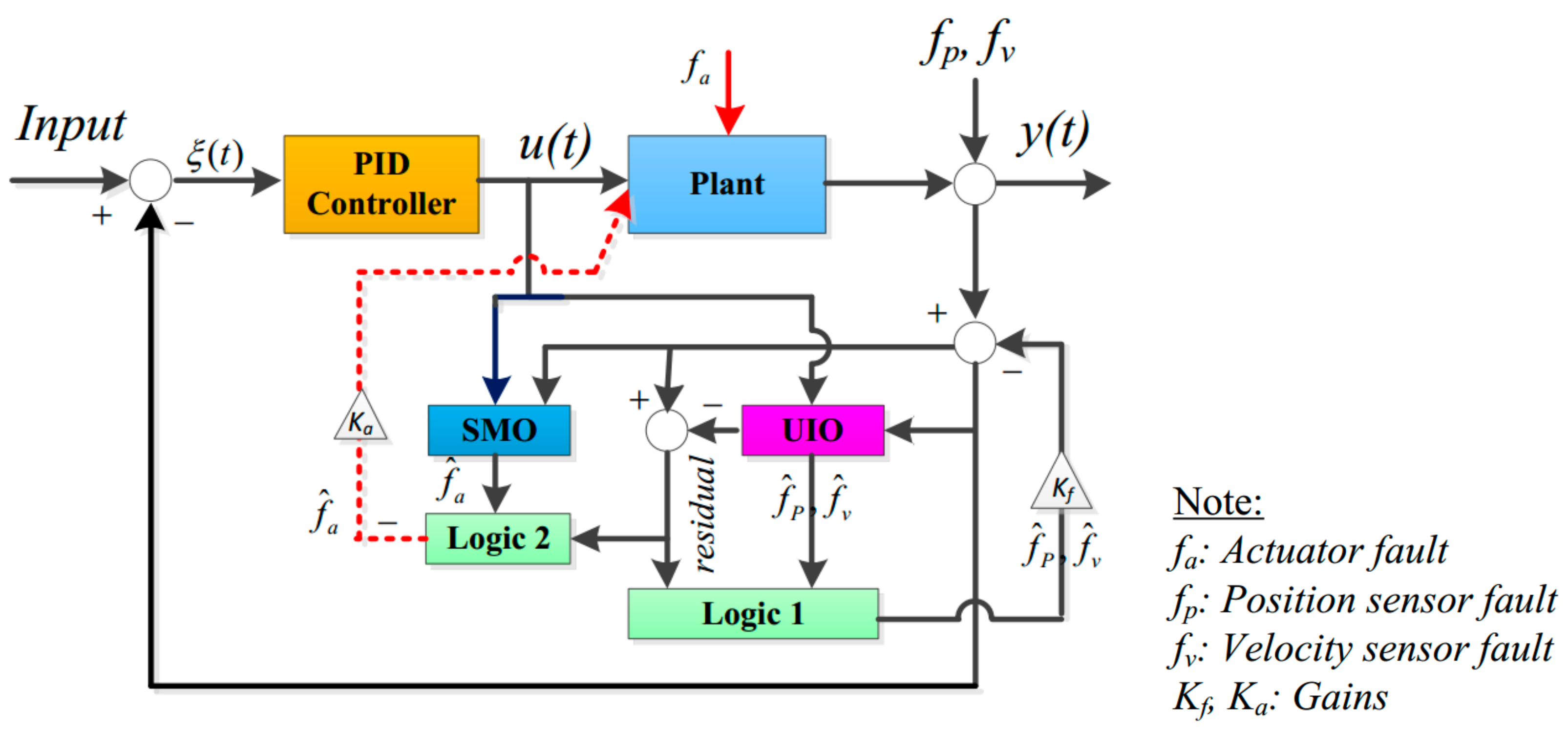
5. Actuator and Sensor Fault-Tolerant Control

5.1. Fault Tolerant Control Based General Residual and the Actuator and Sensor Fault Compensation

Fault-Tolerant Control (FTC) is implemented by compensating the actuator and sensor faults through UIO and SMO models. The residual has been proposed by [34,35,36,37,38], which is calculated as:

$$r=‖y-\widehat{y}‖$$

(81)

The fault compensation process consists of two main processes: fault detection and compensation. The fault detection process involves determining whether a fault has occurred or not, depending on the information of the residual, which means that $r=0$ if $s=0$ without fault and $r\ne 0$ if $s\ne 0$ with fault ($s={\left[\begin{array}{cc}{f}_P^T& f_v^T\end{array}\right]}^T$ or $s=f_a$). The fault isolation process is executed to make a binary decision signal based on the fault detection process. Here, making a binary decision is defined by a logical process that is constructed out of the residual and the threshold value k. The binary decision signal is 0, if $\left|r\right|\le k$, and conversely, this signal is 1, if $\left|r\right|>k$. However, the selection of the coefficient k is realized from the following experience.

5.2. Actuator and Sensor Fault Compensation

FTC-based actuator and sensor fault compensation is designed through residual shown in Figure 2. The main PID controller will operate conventional closed-loop trajectory control.

The actuator compensation signal for the EHA system can be designed as $u_f=K_a{\widehat{f}}_a$, where

$$K_a={\mathsf{\Theta }}^{+}F$$

(82)

The component of the measurement output can be described as:

$$y_c=y-S\left[\begin{array}{c}{\widehat{f}}_p\\ {\widehat{f}}_v\end{array}\right]$$

(83)

The binary decision signal is used to operate a logic process, when it has a value ‘1’, a fault occurs, and the fault compensation is performed. If no fault occurs, the binary decision signal has a value ‘0’ as in [33,34,35,36].

5.3. Evaluating the Control Error Performance

The position tracking error is one of the important factors to evaluate the position tracking controller performance. In this paper, the performance of the position tracking controller PID is proposed. To simplify the calculation, the one-norm ${\mu }_{\xi }$ of a position error vector ${\xi }_y$ is presented as:

$${\mu }_{\xi }=‖{\xi }_y‖$$

(84)

The maximum value of the error ${\xi }_y$ is presented in a period from t₀ to t is given as:

$${\mu }_{\xi \max }=\max {\displaystyle \sum _{t_0}^t‖{\xi }_y‖}$$

(85)

The position tracking error performance using the fault compensation method is computed as:

$$\eta =\left(1-\frac{{\mu }_{\max }}{{\mu }_{\xi \max }}\right)100\%$$

(86)

where ${\mu }_{\max }$ is the maximum value of the obtained error when applying for fault compensation in a period from t₀ to t.

6. Results

6.1. The Parameters of the MMP System

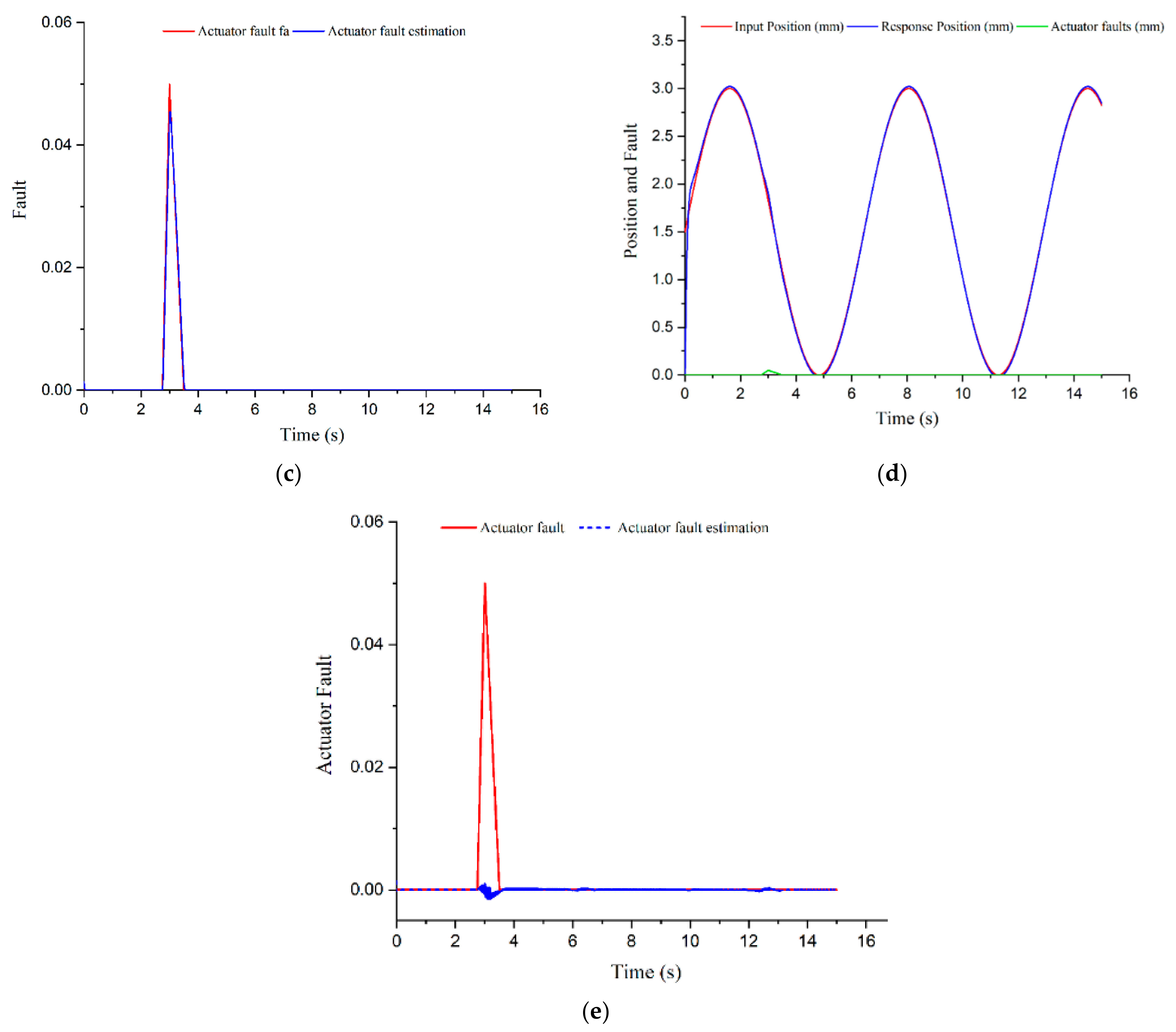
The basic parameters of the MMP system are shown in

Table 1. Basic parameters of the EHA system.

Components	Values	Units
Ah	0.0013	m2
Ar	9.4 × 10−4	m2
Vch	2.09 × 10−4	m3
Vcr	4.0065 × 10−5	m3
mp	10	kg
βe	2.9 × 108	Pa
Ksp	2383	Nm
Dp	3.5 × 10-6	m3

. Following these parameters, the received data are shown as [33]:

$$\mathsf{\Phi }=\left[\begin{array}{cc}0& 1\\ -554.57& -1464.2857\end{array}\right]; \mathsf{\Theta }=\left[\begin{array}{c}0\\ 1.857\hspace{0.17em}\hspace{0.17em}{10}^{-4}\end{array}\right];\hspace{0.17em}\mathsf{\Upsilon }=[1\hspace{0.17em}\hspace{0.17em}\hspace{0.17em}\hspace{0.17em}0];\hspace{0.17em}\mathsf{\Psi }=\left[\begin{array}{c}0.25\hspace{0.17em}{10}^{-4}\hspace{0.17em}\\ -1.42861\hspace{0.17em}{10}^{-4}\end{array}\right]$$

6.2. Actuator Fault

6.2.1. Actuator Fault Estimation

The basic parameters of the MMP system utilized in the observer model are as follows:

$${\mathsf{\Phi }}_z=\left[\begin{array}{ccc}0& 1& 0\\ -554.57& -1464.286& 0\\ 0& 0& 0\end{array}\right];{\mathsf{\Theta }}_z=\left[\begin{array}{c}0\\ 1.857\hspace{0.17em}{10}^{-4}\\ 0\end{array}\right];{\mathsf{\Upsilon }}_z=\left[\begin{array}{ccc}0& 1& 0\\ 0& 0& 1\end{array}\right];\hspace{0.17em}\hspace{0.17em}{F}_z=\left[\begin{array}{c}\mathsf{\Psi }\\ 0.001\end{array}\right]$$

A non-singular transformation matrix can be selected as:

$$T_{\mathsf{\Upsilon }}=\left[\begin{array}{ccc}-0.707& -0.707& -0.707\\ 1& 0& 1\\ 0& 1& 0\end{array}\right]$$

With Lipschitz constant λ = 0.5, and ${\alpha }_0=0.2$, we can solve Equation (26) using the LMI algorithm for $U_{11},\hspace{0.17em}{U}_{12},\hspace{0.17em}{U}_0,\hspace{0.17em}{\mathsf{\Phi }}_0$, and $U$; if the solution is feasible, the results are obtained as follows:

$$\begin{gathered} {\alpha }_1=0.52876;\hspace{0.17em}\mu =0.0002;\hspace{0.17em}{U}_{11}=4.145\hspace{0.17em}{10}^{-3};U_{12}=\left[\begin{array}{cc}-5.09\hspace{0.17em}{10}^{-11}& -5.308\hspace{0.17em}{10}^{-4}\end{array}\right]; \\ {U}_0=\left[\begin{array}{cc}1.589\hspace{0.17em}{10}^{-1}& -1.609\hspace{0.17em}{10}^{-13}\\ -1.609\hspace{0.17em}{10}^{-13}& \hspace{0.17em}1.202\hspace{0.17em}{10}^{-3}\end{array}\right];\hspace{0.17em}{\mathsf{\Phi }}_0=\left[\begin{array}{cc}-5.3735& -7.60078\hspace{0.17em}{10}^{-10}\\ -5.62\hspace{0.17em}{10}^{-8}& \hspace{0.17em}-7.5075\hspace{0.17em}{10}^2\end{array}\right] \\ U=\left[\begin{array}{ccc}4.145\hspace{0.17em}{10}^{-3}& -5.091\hspace{0.17em}{10}^{-11}& -5.308\hspace{0.17em}{10}^{-4}\\ -5.091\hspace{0.17em}{10}^{-11}& 1.58945\hspace{0.17em}{10}^{-1}& 6.3584\hspace{0.17em}{10}^{-10}\\ -5.308\hspace{0.17em}{10}^{-4}& 6.3584\hspace{0.17em}{10}^{-10}& -7.5075\hspace{0.17em}{10}^2\end{array}\right] \end{gathered}$$

The equation of the commanded input is given as:

$$y_r=1.5\sin \left(0.975t\right)+1.5$$

(87)

We assume that the actuator fault $f_a(t)$ is given as:

$$f_a(t)=\left\{\begin{array}{ll}0& \hspace{0.17em}if\hspace{0.17em}\hspace{0.17em}\hspace{0.17em}t\le 2.5\\ 0.05t-11/80& \hspace{0.17em}if\hspace{0.17em}\hspace{0.17em}\hspace{0.17em}2.5\le t\le 3\\ -0.05t+7/40& \hspace{0.17em}if\hspace{0.17em}\hspace{0.17em}\hspace{0.17em}3\le t\hspace{0.17em}\le 3.5\hspace{0.17em}\\ 0& \hspace{0.17em}if\hspace{0.17em}\hspace{0.17em}\hspace{0.17em}t>3.5\end{array}\right.$$

(88)

6.2.2. Simulation Results for Actuator Fault

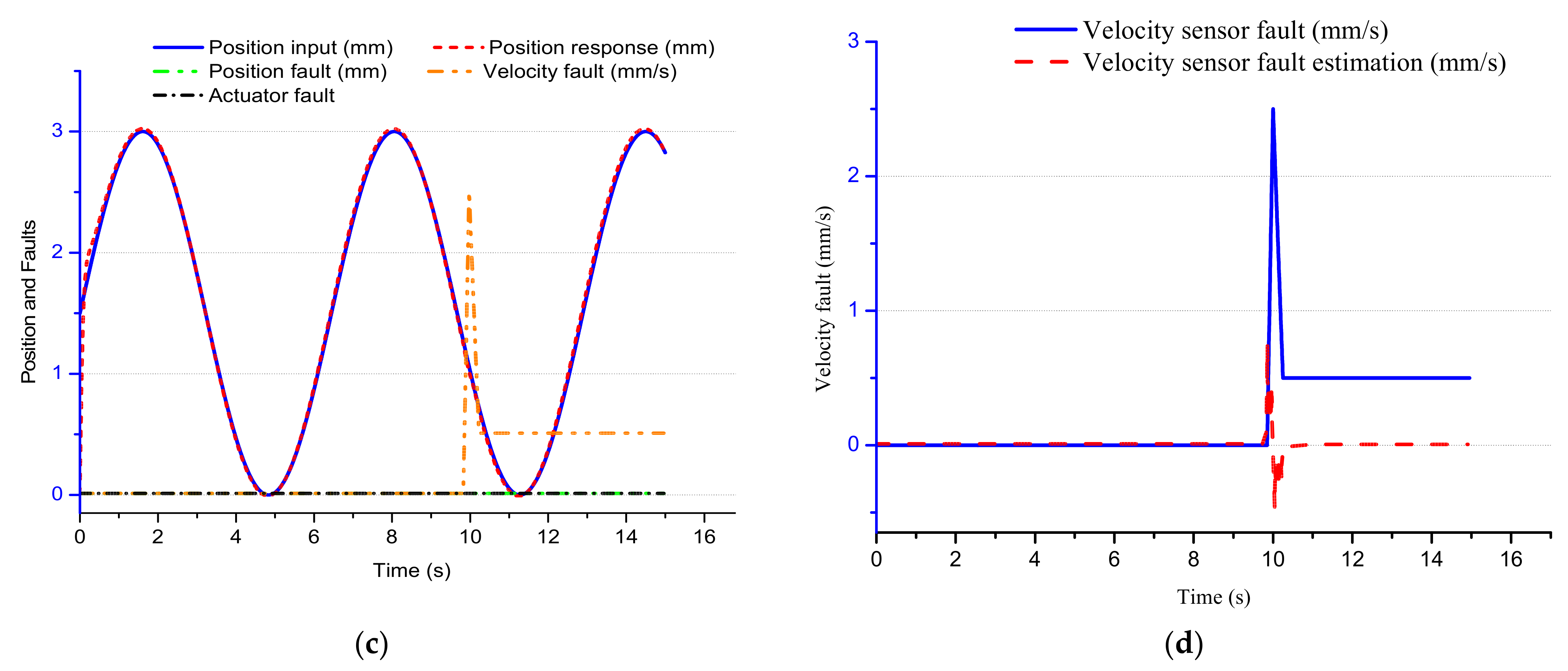
In this section, we consider the influence of actuator fault $f_a$ on the EHA system that is given by Equation (88) in Matlab/Simulink environment with a sinusoidal input signal, as shown in Equation (87). On the other hand, the actuator error compensation-based FTC process is applied through the actuator fault estimation of the SMO model. As shown in Figure 3a, the simulation results obtained from the EHA system for the no-fault case demonstrate that the system works well, using the traditional PID controller. From Figure 3b–e, the negative effects of actuator fault on the position response and actuator fault estimation with and without actuator fault compensation are described respectively. Figure 3b shows that the position feedback signal (blue line) is adversely affected by the actuator fault (green line), and Figure 3c shows an increased efficiency of the SMO algorithm in estimating the actuator fault. At the same time, the feedback signal affected by the actuator fault is also effectively handled by the FTC compensation algorithm, as illustrated in Figure 3d,e.

6.3. Sensor Fault

6.3.1. Sensor Fault Estimation

We assume that the position sensor fault $f_p(t)$ is given as:

$$f_a(t)=\left\{\begin{array}{ll}0& if\hspace{0.17em}\hspace{0.17em}\hspace{0.17em}t\le 5.65\\ 0.05\sin (7.5t)+0.50025& if\hspace{0.17em}\hspace{0.17em}\hspace{0.17em}5.65\le t\le 6.71015\hspace{0.17em}\\ 0.53& if\hspace{0.17em}\hspace{0.17em}\hspace{0.17em}6.71015\hspace{0.17em}\le t\le 11.79\\ 0.918t-10.6373& if\hspace{0.17em}\hspace{0.17em}\hspace{0.17em}11.79\le t\le 12.35\\ 22.3125-1.75t& if\hspace{0.17em}\hspace{0.17em}\hspace{0.17em}12.35\le t\le 12.7\\ 0.9t-11.3425& if\hspace{0.17em}\hspace{0.17em}\hspace{0.17em}12.7\le t\le 13.05\hspace{0.17em}\end{array}\right.$$

(89)

Suppose the position velocity fault $f_s(t)$ can be described as:

$$f_v(t)=\left\{\begin{array}{ll}0& \hspace{1em}if\hspace{0.17em}0\le t\le 9.85\\ 2.5t-197/8& \hspace{1em}if\hspace{0.17em}9.85\le t\le 10\\ 165/8\hspace{0.17em}-2t& \hspace{1em}if\hspace{0.17em}10\le t\le 10.25\\ 0.5& \hspace{1em}if\hspace{0.17em}t<20\end{array}\right.$$

Assume that we choose the Lipschitz constant ${\zeta }_s=5\hspace{0.17em}$ and positive coefficients $r=\alpha =\epsilon =0.1$, and $\mu =0.2$ by applying LMI algorithm. We can solve matrices $P;\hspace{0.17em} Q$ and $L$ by (70) and (71) if the solution is feasible, then we obtain the results as follows:

$$\begin{gathered} P=\left[\begin{array}{cccc}7.8101& 0.0057& 8.0832& -0.0546\\ 0.0057& 0.0982& -0.0243& 0.0247\\ 8.0832& -0.0243& 8.3963& -0.0524\\ -0.0546& 0.0247& -0.0524& 0.0363\end{array}\right]; Q=\left[\begin{array}{cc}51.9785& -99.8584\\ 0.3824& -1.1467\\ 80.7266& -5.8503\\ 76.1973& 108.0462\end{array}\right]; \\ L=\left[\begin{array}{cc}225.1138& -111.2963\\ -725.6963& -877.7046\\ -192.6286& 120.0004\\ 2654.0404& 3580.4874\end{array}\right] \end{gathered}$$

6.3.2. Simulation Results for Sensor Faults

• Position Fault

A consideration of the effects of the position and velocity sensor (PVS) faults on the EHA system in the case of the sinusoidal input signal is also presented, as given in Equation (87). An FTC process using PVS error compensation is also considered through the PVS error estimation of the UIO model, as shown in Figure 2. In Figure 4a and Figure 5a, the position feedback signal (red line) is affected by position sensor fault (green line) and sensor fault (orange line). Here, PVS fault estimation is effectively executed under the support of the UIO model, which is shown in Figure 4b and Figure 5b. By applying the FTC compensation algorithm, the feedback signal under the negative impact of the position sensor fault (Figure 4c,d) and velocity sensor fault (Figure 5c,d) is handled, respectively.

• Velocity Sensor Fault

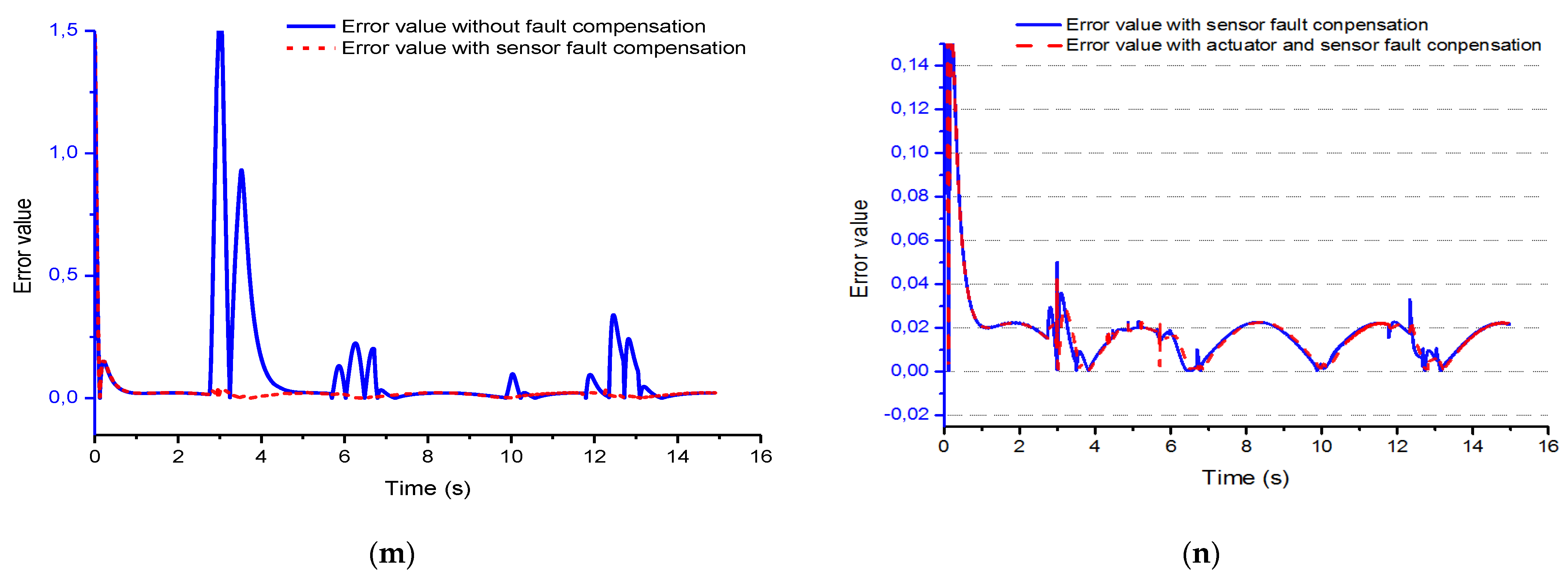
• Position sensor, velocity sensor, and actuator faults

In this section, the impact of three components (i.e., actuator fault f_a (AF), position sensor fault f_p, and velocity sensor fault f_v) on the EHA system is under consideration to minimize the effect of noises, disturbances, and uncertain kinetic parameters. Specifically, an FTC process of compensating for AF and PVS is suggested based on a sequential combination of the AF and PVS estimation using the SMO and UOI models, as shown in Figure 2. In Figure 6a, the position feedback signal (red line) of the system is simultaneously affected by three fault components: actuator fault (black line), position sensor fault (green line), and velocity sensor fault (orange line). Thanks to the estimated errors shown in Figure 6b–d, we can easily compute the estimated actuator error difference affected by the position sensor and velocity fault, which is illustrated in Figure 6b. Figure 6c.d clearly show the effect of actuator fault on the estimated sensor fault. Here, the controlled error signal is evaluated in Figure 6e, and the error magnitude is shown in Figure 6f. In addition, to evaluate the performance of the proposed control method FTC under the impact of the aforesaid faults, the control error is shown in Figure 6g when sensor fault compensation is applied, and the error level is evaluated in Figure 6h.

By applying the closed-loop control system with FTC to the actuator fault, and sensor fault compensation method as shown in Figure 2, the effects of the fault are greatly reduced, as shown in Figure 6i. Thanks to this FTC error compensation technology, the estimation errors are almost eliminated and approximate to zero, as described in Figure 6j,k,l. The control error shown in Figure 6m corresponds to the case where actuator and sensor fault compensation is applied, as well as the evaluated value of the fault in Figure 6n.

Here, μ_ξmax, μ_sξmax, and μ_asξmax are respectively the maximum values of the errors when using the PID controller, the sensor fault compensation method, and the actuator-sensor fault compensation method, respectively; η_sξ, and η_asξ are fault efficiencies achieved by the sensor fault compensation method and actuator-sensor fault compensation method.

Table 2. An evaluation of the error performance using the fault compensation compared to the PID controller.

Time Period	Error Value			Error Performance ηξ
	μξmax	μsξmax	μasξmax	ηsξ	ηasξ
From 1 s to 5 s	1.634545	0.049849	0.042386	96.95026	97.40684
From 5 s to 8 s	0.224818	0.022824	0.022793	89.84799	89.86136
From 8 s to 11 s	0.099249	0.02229	0.022377	77.54112	77.45363
From 11 s to 15 s	0.340294	0.032808	0.022219	90.35901	93.47057

shows that the efficiency of control error is approximately 96.95% when using the sensor fault compensation method, compared to the PID controller in the period from 1s to 5s. Moreover, when we use the actuator-sensor fault compensation method, the efficiency reaches 97.41% and the result is, therefore, better than the sensor fault compensation method. In addition, in the periods that the system suffers from position sensor fault (i.e., 5 s–8 s and 11 s–15 s), although the performance of the fault compensation method is much more efficient than the PID method, the actuator-sensor fault compensation method still achieves higher efficiency than the sensor fault compensation method. In the period from 8s to 11s, although the speed error adversely affects the system, the efficiency is also relatively high at about 77.5%, and the efficiency of the actuator-sensor fault compensation and sensor fault compensation methods is the same in this case. Based on the above results, we can see that the actuator-sensor fault compensation method is more effective than the sensor fault compensation method presented previously [33].

With the implementation of powerful control methods, the impact of the control input signal is very large when the input signal is very high, as shown in [44,45]. However, when the control speed is in the allowable limits (no more than 25 mm/s), a fault compensation based robust fault-tolerant control method can greatly reduce the effects of faults after each closed control loop. In practice, the sensor fault compensation algorithm has been proved that it can successfully minimized the sensor faults under various conditions [33].

7. Conclusions

Recently, the EHA has been widely applied in many applications, from industry to agriculture. Although this system has a lot of advantages, for it to better meet practical applications, some disadvantages of the system, including disturbances, internal leakage fault, sensor fault, and the dynamic uncertain equation components of the system that make the system unstable and unsafe, need to be overcome, especially eliminating the influence of noise on the system operation. In this paper, an actuator-sensor fault compensation was proposed. To implement the proposed solution, we developed the Lyapunov-based SMO to estimate the faults that come from the payload variations and unknown friction nonlinearities. Next, we estimated the sensor faults thanks to Lyapunov analysis-based UIO model. Then, we applied actuator-sensor compensation faults to minimize the estimated faults. Simulation results demonstrated that this method achieved very high efficiency, despite the influence of noises. Obviously, this result is superior to the traditional PID method and even better than an advanced method, namely the sensor error compensation method. The above analysis results significantly contributed to improving the performance of EHA systems in practice.

References

1. Yao, J.; Yang, G.; Jiao, Z. High dynamic feedback linearization control of hydraulic actuators with backstepping. Proc. Inst. Mech. Eng. Part I J. Syst. Control. Eng. 2015, 229, 728–737. [Google Scholar] [CrossRef]
2. Wonohadidjojo, D.M.; Kothapalli, G.; Hassan, M.Y. Position Control of Electro-hydraulic Actuator System Using Fuzzy Logic Controller Optimized by Particle Swarm Optimization. Int. J. Autom. Comput. 2013, 10, 181–193. [Google Scholar] [CrossRef] [Green Version]
3. Feng, L.; Yan, H. Nonlinear Adaptive Robust Control of the Electro-Hydraulic Servo System. Appl. Sci. 2020, 10, 4494. [Google Scholar] [CrossRef]
4. Huang, J.; An, H.; Yang, Y.; Wu, C.; Wei, Q.; Ma, H. Model Predictive Trajectory Tracking Control of Electro-Hydraulic Actuator in Legged Robot With Multi-Scale Online Estimator. IEEE Access 2020, 8, 95918–95933. [Google Scholar] [CrossRef]
5. Skarpetis, M.G.; Koumboulis, F.N. Robust PID controller for electro—Hydraulic actuators. In Proceedings of the 2013 IEEE 18th Conference on Emerging Technologies & Factory Automation (ETFA), Cagliari, Italy, 10–13 October 2013; pp. 1–5. [Google Scholar] [CrossRef]
6. Ishak, N.; Tajjudin, M.; Ismail, H.; Rahiman, M.H.F.; Sam, Y.M.; Adnan, R. PID Studies on Position Tracking Control of an Electro-Hydraulic Actuator. Int. J. Control. Sci. Eng. 2012, 2, 120–126. [Google Scholar] [CrossRef] [Green Version]
7. Kim, H.M.; Park, S.H.; Song, J.H.; Kim, J.S. Robust Position Control of Electro-Hydraulic Actuator Systems Using the Adaptive Back-Stepping Control Scheme. Proc. Inst. Mech. Eng. Part I J. Syst. Control. Eng. 2010, 224, 737–746. [Google Scholar] [CrossRef]
8. Ji, X.; Wang, C.; Zhang, Z.; Chen, S.; Guo, X. Nonlinear adaptive position control of hydraulic servo system based on sliding mode back-stepping design method. Proc. Inst. Mech. Eng. Part. I J. Syst. Control. Eng. 2021, 235, 474–485. [Google Scholar] [CrossRef]
9. Li, Z.; Xing, K. Application of fuzzy PID controller for electro-hydraulic servo position control system. In Proceedings of the 2017 3rd IEEE International Conference on Control Science and Systems Engineering (ICCSSE), Beijing, China, 17–19 August 2017; pp. 158–162. [Google Scholar] [CrossRef]
10. Do, T.C.; Tran, D.T.; Dinh, T.Q.; Ahn, K.K. Tracking Control for an Electro-Hydraulic Rotary Actuator Using Fractional Order Fuzzy PID Controller. Electronics 2020, 9, 926. [Google Scholar] [CrossRef]
11. Hu, X.; Al-Ani, D.; Habibi, S. A new Sliding Mode Controller for Electro-Hydraulic Actuator (EHA) applications. In Proceedings of the 2015 International Workshop on Recent Advances in Sliding Modes (RASM), Istanbul, Turkey, 9–11 April 2015; pp. 1–7. [Google Scholar] [CrossRef]
12. Shi, Z.; Tang, Z.; Pei, Z. Sliding Mode Control for Electrohydrostatic Actuator. Hindawi Publ. Corp. J. Control. Sci. Eng. 2014, 2014, 481970. [Google Scholar] [CrossRef] [Green Version]
13. Thomas, A.T.; Parameshwaran, R.; Sathiyavathi, S.; Starbino, A.V. Improved Position Tracking Performance of Electro Hydraulic Actuator Using PID and Sliding Mode Controller. IETE J. Res. 2019, 1–13. [Google Scholar] [CrossRef]
14. Tri, N.M.; Nam, D.N.C.; Park, H.G.; Ahn, K.K. Trajectory control of an electro hydraulic actuator using an iterative backstepping control scheme. Mechatronics 2014, 29, 96–102. [Google Scholar] [CrossRef]
15. Ahn, K.K.; Doan, N.; Jin, M. Adaptive Backstepping Control of an Electrohydraulic Actuator. Mechatronics. IEEE ASME Trans. 2014, 19, 987–995. [Google Scholar] [CrossRef]
16. Guo, Q.; Shi, G.; Wang, D.; He, C. “Neural network–based adaptive composite dynamic surface control for electro-hydraulic system with very low velocity. Proc. Inst. Mech. Eng. Part. I J. Syst. Control. Eng. 2017, 231, 867–880. [Google Scholar] [CrossRef]
17. Liem, D.T.; Truong, D.Q.; Park, H.G.; Ahn, K.K. A feedforward neural network fuzzy grey predictor-based controller for force control of an electro-hydraulic actuator. Int. J. Precis. Eng. Manuf. 2016, 17, 309–321. [Google Scholar] [CrossRef]
18. Zhu, L.; Wang, Z.; Zhou, Y.; Liu, Y. Adaptive Neural Network Saturated Control for MDF Continuous Hot Pressing Hydraulic System with Uncertainties. IEEE Access 2018, 6, 2266–2273. [Google Scholar] [CrossRef]
19. Li, W.; Shi, G. RBF Neural Network Sliding Mode Control for Electro Hydraulic Servo System. Chin. Hydraul. Pneum. 2019, 109–114. [Google Scholar]
20. Ossmann, D.; van der Linden, F.L.J. Advanced sensor fault detection and isolation for electro-mechanical flight actuators. In Proceedings of the 2015 NASA/ESA Conference on Adaptive Hardware and Systems (AHS), Montreal, QC, Canada, 15–18 June 2015; pp. 1–8. [Google Scholar] [CrossRef] [Green Version]
21. Mitra, D.; Halder, P.; Mukhopadhyay, S. Improved Fault Detection and Isolation of Small Faults using Multiple Residual Generators and Complex Detection Hypotheses: Case Study of an Electro-Hydraulic Aerospace Actuator. In Proceedings of the Annual Conference of the PHM Society, Scottsdale, AZ, USA, 21–22 September 2019. [Google Scholar] [CrossRef]
22. Li, T.; Yu, Y.; Wang, J.; Xie, R.; Wang, X. Sensor fault diagnosis for electro-hydraulic actuator based on QPSO-LSSVR. In Proceedings of the 2016 IEEE Chinese Guidance, Navigation and Control Conference (CGNCC), Nanjing, China, 12–14 August 2016; pp. 1051–1056. [Google Scholar] [CrossRef]
23. Shen, Q.; Jiang, B.; Shi, P. Fault Diagnosis and Fault-Tolerant Control Based on Adaptive Control Approach; Springer International Publishing AG: Cham, Switzerland, 2017; ISBN 978-3-319-52529-7. [Google Scholar]
24. Liu, H.; Liu, D.; Lu, C.; Wang, X. Fault diagnosis of hydraulic servo system using the unscented Kalman filter. Asian J. Control 2014, 16, 1713–1725. [Google Scholar] [CrossRef]
25. Abbaspour, A.; Mokhtari, S.; Sargolzaei, A.; Yen, K.K. A Survey on Active Fault-Tolerant Control Systems. Electronics 2020, 9, 1513. [Google Scholar] [CrossRef]
26. Blanke, M. Fault-tolerant Control Systems. In Advances in Control; Frank, P.M., Ed.; Springer: London, UK, 1999. [Google Scholar] [CrossRef]
27. Nahian, S.A.; Truong, D.Q.; Chowdhury, P.; Das, D.; Ahn, K.K. Modeling and fault tolerant control of an electro-hydraulic actuator. Int. J. Precis. Eng. Manuf. 2016, 17, 1285–1297. [Google Scholar] [CrossRef] [Green Version]
28. Mhaskar, P.; Liu, J.; Christofides, P.D. Fault-Tolerant Process Control: Methods and Applications; Springer: Berlin/Heidelberg, Germany, 2012; ISBN 144714807X. [Google Scholar]
29. Zarei, J.; Shokri, E. Robust sensor fault detection based on nonlinear unknown input observer. Measurement 2014, 48, 355–367. [Google Scholar] [CrossRef]
30. Hashemi, M.; Egoli, A.K.; Naraghi, M.; Tan, C.P. Saturated fault tolerant control based on partially decoupled unknown-input observer: A new integrated design strategy. IET Control Theory Appl. 2019, 13, 2104–2113. [Google Scholar] [CrossRef]
31. Oghbaee, A.; Shafai, B.; Nazari, S. Complete characterisation of disturbance estimation and fault detection for positive systems. IET Control Theory Appl. 2018, 12, 883–891. [Google Scholar] [CrossRef]
32. Amrane, A.; Larabic, A.; Aitouche, A. Unknown input observer design for fault sensor estimation applied to induction machine. Math. Comput. Simul. 2020, 167, 415–428. [Google Scholar] [CrossRef]
33. Tan, N.V.; Cheolkeun, H. Sensor Fault-Tolerant Control Design for Mini Motion Package Electro-Hydraulic Actuator. Processes 2019, 7, 89. [Google Scholar]
34. Tan, N.V.; Cheolkeun, H. Experimental Study of Sensor Fault-Tolerant Control for an Electro-Hydraulic Actuator Based on a Robust Nonlinear Observer. Energies 2019, 12, 4337. [Google Scholar] [CrossRef] [Green Version]
35. Zhang, K.; Jiang, B.; Shi, P.; Cocquempot, V. Observer-Based Fault Estimation Techniques; Springer International Publishing: Berlin/Heidelberg, Germany, 2018; ISBN 978-3-319-67491-9. [Google Scholar]
36. Liu, X.; Gao, Z.; Zhang, A. Robust Fault Tolerant Control for Discrete-Time Dynamic Systems with Applications to Aero Engineering Systems. IEEE Access 2018, 6, 18832–18847. [Google Scholar] [CrossRef]
37. Gao, S.; Ma, G.; Guo, Y.; Zhang, W. Augmented System Observer-based Robust Fault-estimation Scheme for Nonlinear Systems. In Proceedings of the 2021 40th Chinese Control Conference (CCC), Shanghai, China, 26–28 July 2021; pp. 4350–4355. [Google Scholar] [CrossRef]
38. Noura, H.; Theilliol, D.; Ponsart, J.C.; Chamseddine, A. Fault-Tolerant Control. Systems Design and Practical Applications; Michael, J.G., Michael, A.J., Eds.; Springer: Dordrecht, The Netherlands; Heidelberg, Germany; London, UK; New York, NY, USA, 2009; ISBN 978-1-84882-652-6. [Google Scholar] [CrossRef]
39. Zhang, W.; Wang, Z.; Raïssi, T.; Wang, Y.; Shen, Y. A state augmentation approach to interval fault estimation for descriptor systems. Eur. J. Control 2020, 51, 19–29. [Google Scholar] [CrossRef]
40. Alwi, H.; Edwards, C.; Tan, C.P. Fault Detection and Fault-Tolerant Control Using Sliding Modes. In Advances in Industrial Control; Springer: London, UK, 2011. [Google Scholar] [CrossRef]
41. Chaves, E.R.Q.; de ADantas, A.F.O.; Maitelli, A.L. Unknown Input Observer-based Actuator and Sensor Fault Estimation Technique for Uncertain Discrete Time Takagi-Sugeno Systems. Int. J. Control. Autom. Syst. 2020, 19, 2444–2454. [Google Scholar] [CrossRef]
42. Yang, J.; Zhu, F.; Wang, X.; Bu, X. Robust sliding-mode observer-based sensor fault estimation, actuator fault detection and isolation for uncertain nonlinear systems. Int. J. Control Autom. Syst. 2015, 13, 1037–1046. [Google Scholar] [CrossRef]
43. Li, S.; Wang, H.; Aitouche, A.; Christov, N. Sliding mode observer design for fault and disturbance estimation using Takagi–Sugeno model. Eur. J. Control. 2018, 44, 114–122. [Google Scholar] [CrossRef]
44. Kaheni, M.; Zarif, M.H.; Kalat, A.A.; Chisci, L. Robust feedback linearization for input-constrained nonlinear systems with matched uncertainties. In Proceedings of the IEEE 2018 17th European Control Conference (ECC), Limassol, Cyprus, 12–15 June 2018; pp. 2947–2952. [Google Scholar] [CrossRef]
45. Kaheni, M.; Hadad Zarif, M.; Akbarzadeh Kalat, A.; Chisci, L. Radial pole path approach for fast response of affine constrained nonlinear systems with matched uncertainties. Int. J. Robust Nonlinear Control 2020, 30, 142–158. [Google Scholar] [CrossRef]
Figure 1. Block diagram of an electro-hydraulic actuator EHA system [14].
Electronics 10 02774 g001
Figure 2. Scheme for fault-tolerant control based on actuator and sensor fault compensation.
Electronics 10 02774 g002
Figure 3. Simulation results of EHA system under the actuator fault impact. (a) Without faults. (b) Position response for the case without actuator fault compensation. (c) Actuator fault estimation for the case without actuator fault compensation. (d) Position response for the case with actuator fault compensation. (e) Actuator fault estimation for the case with actuator fault compensation.
Electronics 10 02774 g003aElectronics 10 02774 g003b
Figure 4. Simulation results of EHA system under the position sensor fault impact. (a) Position response for the case without position sensor fault compensation. (b) Position sensor fault estimation for the case without position sensor fault compensation. (c) Position response for the case with position sensor fault compensation. (d) Position sensor fault estimation for the case with position sensor fault compensation.
Electronics 10 02774 g004aElectronics 10 02774 g004b
Figure 5. Simulation results of EHA system under the velocity sensor fault impact. (a) Position response for the case of only velocity sensor fault ( f p = 0 ; f a = 0 ) . (b) Velocity fault estimation for the case without velocity sensor fault compensation. (c) Position response for the case with velocity sensor fault compensation. (d) Velocity fault estimation for the case with velocity sensor fault compensation.
Electronics 10 02774 g005aElectronics 10 02774 g005b
Figure 6. Simulation results of EHA system under the impact of the actuator fault, the position, and velocity sensor fault. (a) Position response for the case without compensation of ( f a , f P , f v ) faults. (b) Actuator fault estimation for the case without compensation of ( f a , f P , f v ) faults. (c) Position sensor fault estimation for the case without compensation of ( f a , f P , f v ) faults. (d) Velocity fault estimation for the case without compensation of ( f a , f P , f v ) faults. (e) Control error for the case without ( f a , f P , f v ) fault compensation. (f) Control error evaluation for the case without ( f a , f P , f v ) fault compensation. (g) Control error for the case with ( f P , f v ) fault compensation. (h) The obtained error evaluation for the case with ( f P , f v ) fault compensation. (i) Position response for the case ( f a , f P , f v ) fault compensation. (j) Actuator fault estimation for the case ( f a , f P , f v ) fault compensation. (k) Position fault estimation for the case ( f a , f P , f v ) fault compensation. (l) Velocity fault estimation for the case ( f a , f P , f v ) fault compensation. (m) The obtained error evaluation for the case without compensation of ( f a , f P , f v ) faults. (n) The obtained error evaluation for the case with compensation of ( f a , f P , f v ) faults.
Electronics 10 02774 g006aElectronics 10 02774 g006bElectronics 10 02774 g006c