Article

Model Predictive Current Control with Fixed Switching Frequency and Dead-Time Compensation for Single-Phase PWM Rectifier

1
New Energy Research Center, School of Electric Power, South China University of Technology, Guangzhou 510640, China
2
Guangdong Key Laboratory of Clean Energy Technology, School of Electric Power, South China University of Technology, Guangzhou 510640, China
*
Author to whom correspondence should be addressed.
Electronics 2021, 10(4), 426; https://doi.org/10.3390/electronics10040426
Submission received: 20 January 2021 / Revised: 4 February 2021 / Accepted: 6 February 2021 / Published: 9 February 2021
(This article belongs to the Section Power Electronics)

Abstract

:
The research object of this paper is single-phase PWM rectifier, the purpose is to reduce the total harmonic distortion (THD) of the grid-side current. A model predictive current control (MPCC) with fixed switching frequency and dead-time compensation is proposed. First, a combination of an effective vector and two zero vectors is used to fix the switching frequency, and a current prediction equation based on the effective vector’s optimal action time is derived. The optimal action time is resolved from the cost function. Furthermore, in order to perfect the established prediction model and suppress the current waveform distortion as a consequence of the dead-time effect, the dead-time’s influence on the switching vector’s action time is analyzed, and the current prediction equation is revised. According to the experimental results, the conclusion is that, firstly, compared with finite-control-set model predictive control, proportional-integral-based instantaneous current control (PI-ICC) scheme and model predictive direct power control (MP-DPC), the proposed MPCC has the lowest current THD. In addition, the proposed MPCC has a shorter execution time than MP-DPC and has fewer adjusted parameters than PI-ICC. In addition, the dead-time compensation scheme successfully suppresses the zero-current clamping effects, and reduce the current THD.

1. Introduction

The traditional rectification technology is an uncontrolled rectification circuit composed of diodes. Its harm is to produce a large number of current harmonics and inject into the grid, thus affecting the power quality, reducing the service life of electronic equipment. Therefore, in recent years, single-phase PWM rectifiers have been extensive utilized in renewable energy generation [1], motor drive systems [2], uninterruptible power supplies [3], and battery energy storage systems. Because it has higher power factor and lower harmonics compared with uncontrolled rectifier.
The performances of PWM rectifiers are largely determined by the control strategy. The strategies are mainly divided into two categories: indirect current control and direct current control. Indirect current control is to control the grid-side current indirectly by controlling the amplitude and phase of the fundamental voltage wave [4], but due to the lack of current feedback, the dynamic response of the system to the current is slow. Therefore, with the increasing requirements for system performances, indirect current control has been unable to meet these requirements and gradually replaced by direct current control. Common direct current control strategies include hysteresis current control [5,6], proportional-integral-based instantaneous current control (PI-ICC) [7], and proportional-resonant-based instantaneous current control (PR-ICC) [8]. Among them, PI-ICC scheme is widely adopted for single-phase PWM rectifiers. This control algorithm is very simple and can make the switching frequency fixed. Its drawback is the difficulty in the calculation and tuning of PI parameters. Other drawbacks are its poor dynamic response performance and the steady-state error of input current. Compared with PI-ICC, PR-ICC can eliminate steady-state error, but it needs to tune more parameters, and the control results are highly sensitive to the parameters [9]. Ref. [10] proposed a data processing scheme based on the harmonic spectrum for Hall current sensors, which helps to improve the accuracy of the sensor. Aiming at the problem of the DC voltage deviation of the grid-connected converter, the Ref. [11] analyzed the control effect of the input voltage feedforward control, and the results show that the control delay will affect the system dynamics.
With the improvement of digital signal processing capabilities, model predictive control (MPC) schemes are applied to power converters. For finite control set MPC (FCS-MPC), its principle is first to establish the prediction model of the converter, then traverse all the predicted values under the switching vectors and compare them with the reference values, and output the optimal switching vector [12,13,14,15]. It is an algorithm for online scrolling optimization of switch vectors. Compared with PI-ICC, FCS-MPC does not need to calculate or tune PI parameters, and has fast dynamic response, and can also contain nonlinear constraints. However, it also has disadvantages such as unfixed switching frequency and large amount of calculation.
FCS-MPC selects only one switching vector to control the converter during the sampling period, resulting in unfixed switching frequency and high total harmonic distortion (THD) of grid-side current [16,17]. For three-phase PWM rectifiers, Ref. [18,19] constructed the cost function according to the error of active power or reactive power and their reference value, calculated the rectified average voltage vector, and then introduced Space Vector Pulse Width Modulation (SVPWM) to realize the fixed switching frequency. Ref. [20] proposed Modulated MPC (M2PC) for three-phase active rectifiers, which also fixed the switching frequency through SVPWM. The difference from Ref. [18,19] is that Ref. [20] built a cost function based on minimizing the current error. Ref. [21] proposed the concept of the effective time of the switching vector and introduced the calculation method of its analytical solution. Ref. [22] improved the model predictive direct power control (MP-DPC) and obtained the optimal action time of the switching vector by deriving the objective function. Ref. [23] derived the switching function based on model predictive control and filtered the switching function to get the fundamental frequency component, and then achieved the fixed switching frequency through pulse width modulation, and in addition, for three-phase three-level converters, as more switching vectors, resulting in large amount of calculation. In order to solve this problem, Ref. [24] proposed the concept of central vector, which can cancel duty cycle calculation, reduce the program calculation time.
MPC schemes have been extensively investigated in three-phase converters, but there are fewer schemes for single-phase converters. Ref. [25] applied FCS-MPC to photovoltaic inverters and proposed a scheme to normalize the units of each variable in the cost function, so that the weight factor is easier to tune. However, the disadvantage is that the switching frequency is not fixed. Ref. [26] analyzed the performance of the FCS-MPC strategy to control the active power and reactive power of the single-phase grid-connected inverter, but the switching frequency was still not fixed. Ref. [27] proposed an MPC scheme without setting weights for single-phase three-level inverters and realized fixed switching frequency control. Ref. [28] proposed an MP-DPC for single-phase PWM rectifiers based on duty cycle optimization, derived the relationship between duty cycle and instantaneous power, and realized fixed switching frequency control. However, this algorithm needs to perform coordinate translation and coordinate transformation on the AC voltage and current first, and then calculate the instantaneous power, which leads to high program complexity and long execution time, which limits the performance of the algorithm.
For circuits with bridge structures such as single-phase PWM rectifiers, there is still a problem, that is, zero-current clamping effects will arise from the addition of dead-time. After adding the dead-time, the current waveform will be distorted at zero crossing, reducing the current sinusoidal degree and increasing the current THD [29,30,31]. However, the above literatures on model predictive control did not consider the impact of dead-time when establishing predictive models, so the established predictive models were not accurate enough. Most dead-time compensation schemes are on the basis of sinusoidal pulse width modulation (SPWM) [32] or SVPWM [33], and the reference voltage vector is modified based on the polarity of the current. For T-type three-level inverters, the Ref. [34] analyzed the influence of the dead-time on the power prediction value based on the model predictive power control, improved the predictive model, and completed the compensation. However, the dead-time compensation algorithm on the basis of MPC for single-phase PWM rectifiers remains to be investigated. In other works, the converter can operate safely without dead-time by adding additional hardware circuit, Ref. [35,36] added an additional freewheeling-current polarity detection circuit.
This paper proposes an MPCC for single-phase PWM rectifiers, which aims to solve the problems of unfixed switching frequency and no dead-time compensation in the FCS-MPC algorithm. The main work and conclusions can be summarized as follows: (i) Firstly, the switching frequency is fixed by selecting an effective vector and two zero vectors in a sampling period. The principle of fixed switching frequency control is analyzed, and the current prediction equation and the calculation formula of the effective vector optimal action time are derived. (ii) Furthermore, the current path during the dead-time is discussed, and the influence of the dead-time on the effective vector and the zero vector is analyzed. In addition, according to the dead-time effect, the current prediction equation is revised. The conclusion are as follows: the proposed MPCC can fix the switching frequency, greatly reduce the current THD, and the dead-time compensation scheme can effectively suppress the zero-clamping current effects, further reducing the current THD.
The contents of each part of this paper are as follows: In Section 2, the structure of single-phase PWM rectifier is analyzed and the mathematical model is established. In Section 3, an MPCC scheme with fixed switching frequency is proposed. On the basis of the Section 3, the Section 4 considers the effect of dead-time to revise the proposed current prediction model. In Section 5, the simulation results are given. In Section 6, the experimental results are compared and analyzed. In Section 7, the conclusions are summarized.

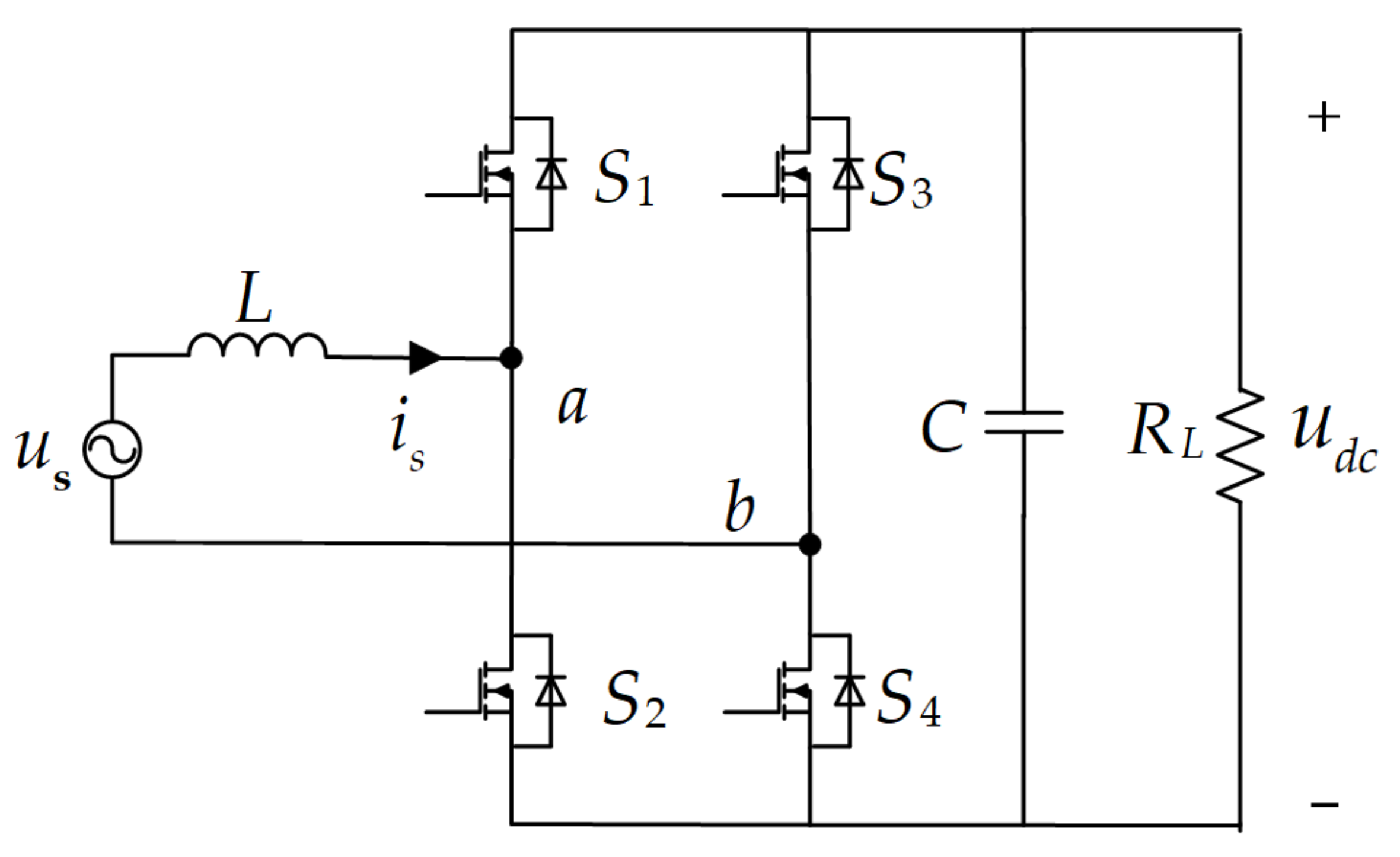
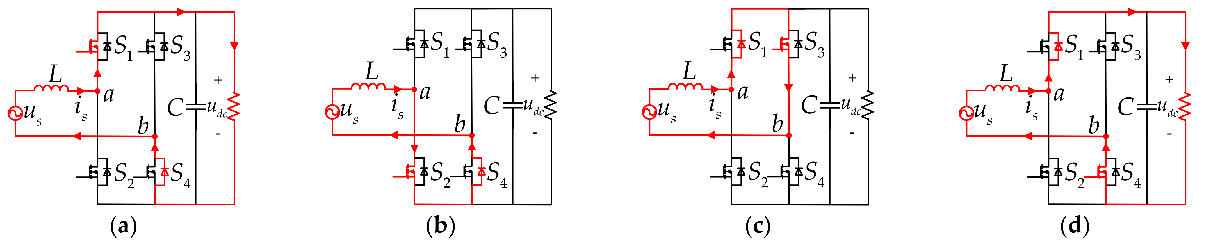
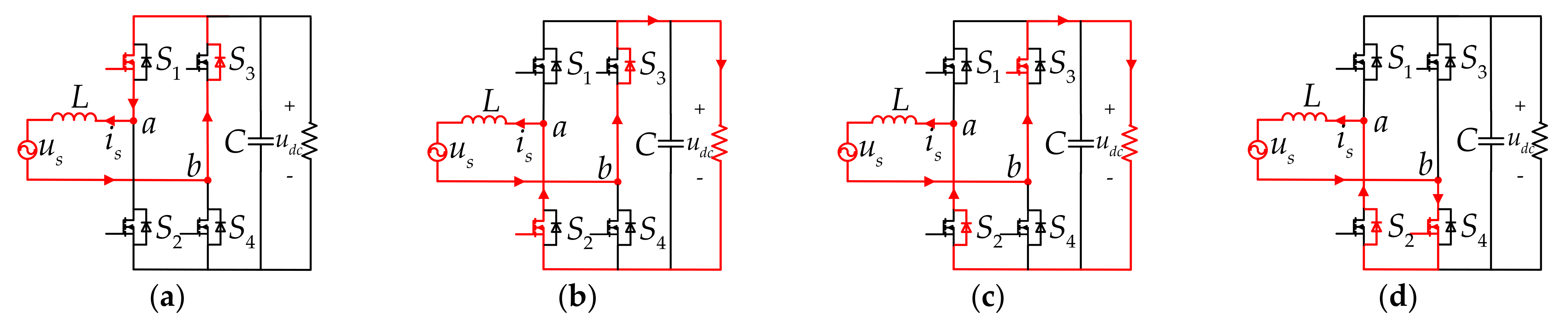
2. Mathematical Model of Single-Phase PWM Rectifiers

The single-phase PWM rectifier consists of a filter inductance, four switches, and a DC-link capacitor, as shown in Figure 1. Where u s represents the input AC voltage, i s represents the input current, L represents the filter inductance, S 1 to S 4 represent four switches, S 1 and S 2 are defined as leg a, S 3 and S 4 are defined as leg b, and C is the DC-link capacitor, R L is the load resistance, and u d c is the DC-link voltage.
It can be concluded from Figure 1 that the voltage equation is
u s = L d i s d t + u a b
where u a b is the input voltage of the rectifier.
There are four switching states of single-phase PWM rectifier, as shown in Table 1.
It can be seen from Table 1 that when S 2 , S 4 or S 1 , S 3 are on at the same time, u a b = 0 , then the switching vectors (1,0,1,0) and (0,1,0,1) are called zero vectors, and the switching vectors (1,0,0,1) and (0,1,1,0) are called effective vectors accordingly.
Define the switch function S a b as
S a b = 1 ( 1 , 0 , 0 , 1 ) 0 ( 1 , 0 , 1 , 0 )   o r   ( 0 , 1 , 0 , 1 ) - 1 ( 0 , 1 , 1 , 0 )  
Then we can get
u a b = S a b u d c
Substituting Equation (3) into Equation (1), and discretizing Equation (1), the difference equation can be obtained as
i s k + 1 = i s k + T s L u s k S a b k u d c
where i s k + 1 is the predicted value of current at instant k + 1 , i s k and u s k are the sampling values of AC voltage and input current at instant k , S a b k is the switching function at instant k , and T s is the sampling period.

3. The Principle of Model Predictive Current Control with Fixed Switching Frequency

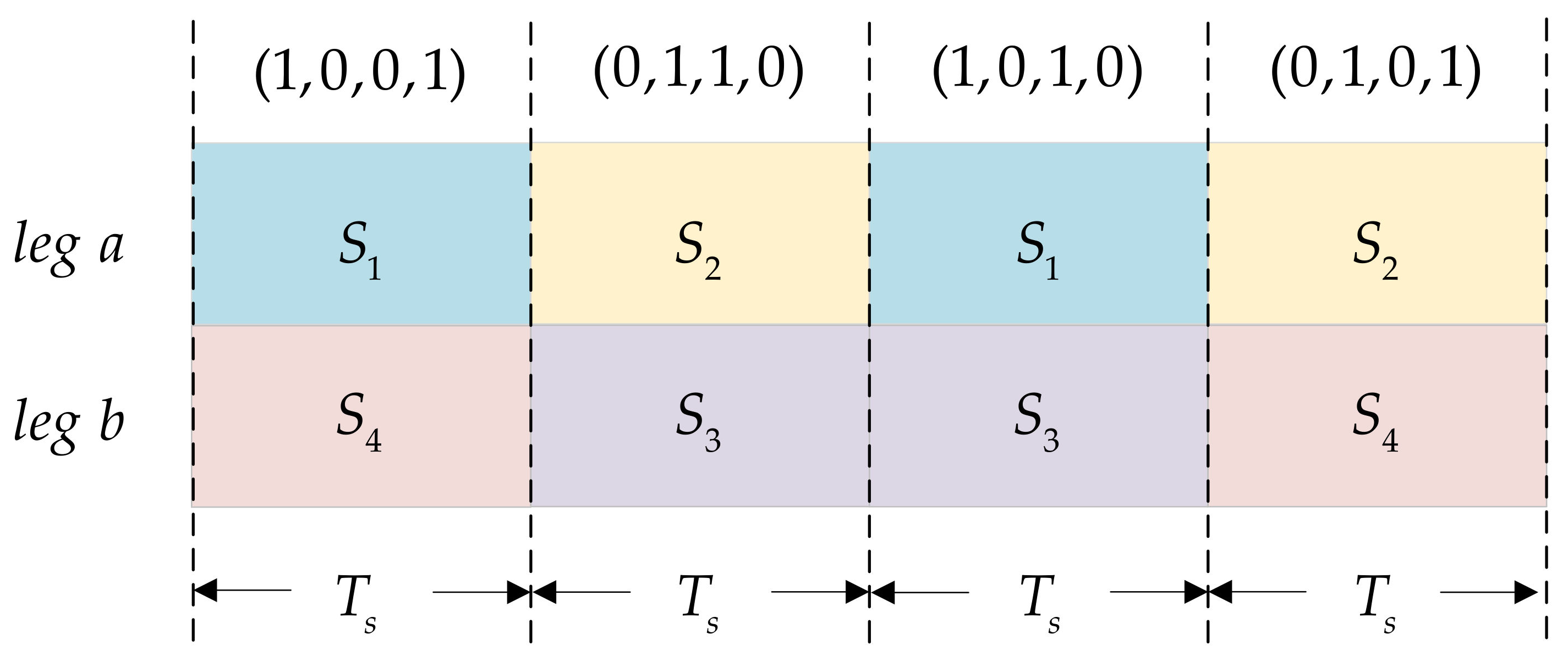
3.1. The Principle of Fixed Switching Frequency Control

FCS-MPC only selects one switching vector in a sampling period; then, there are four kinds of possible switching vectors in a sampling period, as shown in Figure 2.
According to Figure 2, the conduction time of each switch under these switching vectors within a sampling period is shown in Table 2.
Under the control of only one switching vector, the conduction time of each switch can only be T s or 0, that is, the switch is always on or off in a sampling period. Therefore, each switch needs at least two sampling periods to carry out a complete switching action, so the switching frequency does not exceed f s / 2 at most, where f s / 2 is the sampling frequency.
In this paper, a scheme of combining an effective vector and two zero vectors in a sampling period is adopted. Since there are only two types of effective vector and zero vector, there are only two possible switching vector combinations in a sampling period, as shown in Figure 3. Considering the symmetry of the switching vector, the action time of the two zero vectors is equal. The conduction time of each switch is shown in Table 3.
The t o n in Figure 3 and Table 3 represents the action time of the effective vector, 0 < t o n < T s . It can be seen from Table 3 that the conduction time of all switches is controlled between 0 and T s . Therefore, a complete switching action can be carried out within each sampling period, that is, the switching frequency is equal to the sampling frequency, so the switching frequency can be fixed.

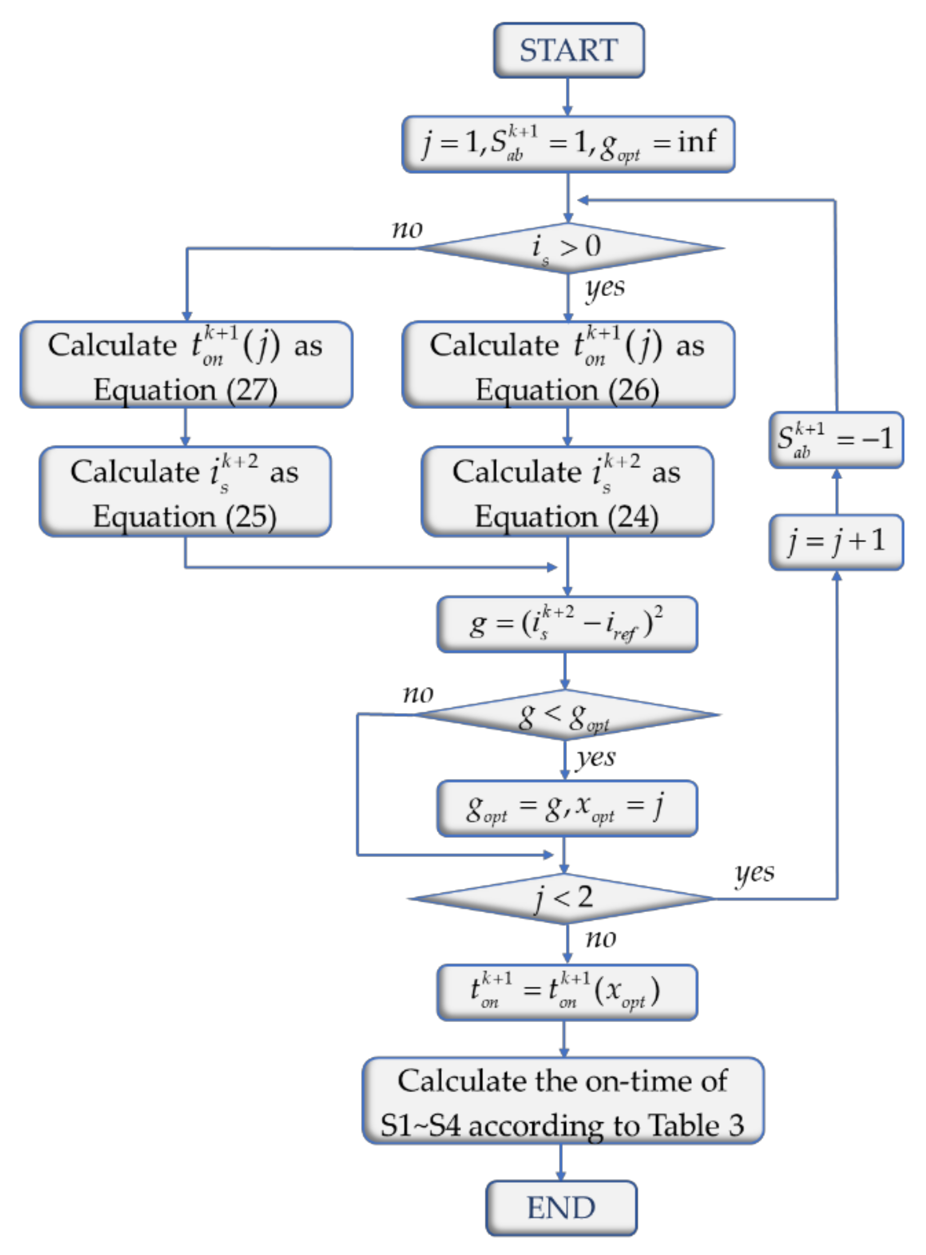
3.2. Current Prediction Equation

Assuming that the action time of the effective vector at instant k is t o n k , so Equation (4) can be changed to
i s k + 1 = i s k + t o n k L u s k S a b k u d c T s t o n k L u s k = i s k + T s L u s k t o n k L S a b k u d c
Due to the sampling time and calculation time in the control system, there is a delay in the output of the controller, which affects the control result. The error caused by the delay can be compensated by predicting the current at instant k + 2.
First, according to Equation (5), we can get
i s k + 2 = i s k + 1 + T s L u s k + 1 t o n k + 1 L S a b k + 1 u d c
Then the current deviations at instant k and k+1 can be expressed as Equations (7) and (8), respectively.
Δ i s k = i s k + 1 i s k = T s L u s k t o n k L S a b k u d c
Δ i s k + 1 = i s k + 2 i s k + 1 = T s L u s k + 1 t o n k + 1 L S a b k + 1 u d c
Due to the high sampling frequency, we can assume that Δ i s k = Δ i s k + 1 , then we get
Δ i s k + 1 = 1 2 Δ i s k + Δ i s k + 1 = 1 2 i s k + 2 i s k
In the same way, we can assume that u s k + 1 u s k = u s k u s k 1 , then we can get
u s k + 1 = 2 u s k u s k 1
Substitute Equations (9) and (10) into (8), then we can get
i s k + 2 = i s k + 2 T s L 2 u s k u s k 1 2 t o n k + 1 L S a b k + 1 u d c
Equation (11) shows the direct relationship between i s k + 2 and i s k , so the process of calculating the intermediate quantity i s k + 1 can be omitted, simplifying the calculation. Then use Equation (11) as the current prediction equation.

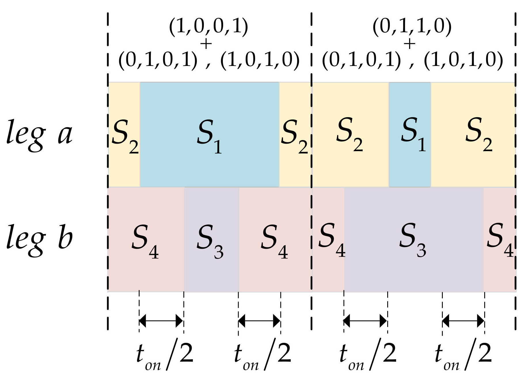
3.3. Cost Function and the Optimal Action Time of the Effective Vector

On the basis of minimizing the error of input current, the cost function is established. There are two optional functions, as shown in the following Equations.
g = i r e f i s k + 2
g = ( i r e f i s k + 2 ) 2
where i r e f is the reference value of the current.
The task of the cost function is to evaluate the closeness between the predicted value and the reference value. The value of the cost function itself has no practical physical significance, and Equations (12) and (13) have the same monotonicity, so their effects are the same. In order to get the optimal action time of the effective vector, the cost function needs to be differentiated, so the differentiable variance function shown in Equation (13) is chosen as the cost function.
By deriving Equation (13) and making its derivative equal to 0, the optimal action time corresponding to the effective vector can be obtained, and the value of cost function can be minimized under this action time.
d g d t o n k + 1 = 0
Substituting Equations (11) and (13) into (14) we can get
t o n k + 1 = L i s k i r e f + 2 T s L 2 u s k u s k 1 2 S a b k + 1 u d c
When t o n k + 1 is calculated to be greater than T s , let it be equal to T s ; when t o n k + 1 is calculated to be less than 0, let it be equal to 0.
The control structure of the PLL is shown in Figure 4. First, the AC voltage is passed through a second-order generalized integrator (SOGI) to obtain a set of orthogonal components u s α , u s β .
The DC components u s d and u s q can be obtained after coordinate transformation of u s α and u s β , and then the voltage phase θ can be obtained by controlling u s q = 0 through PI controller. In Figure 4, ω 0 is the initial angular frequency.

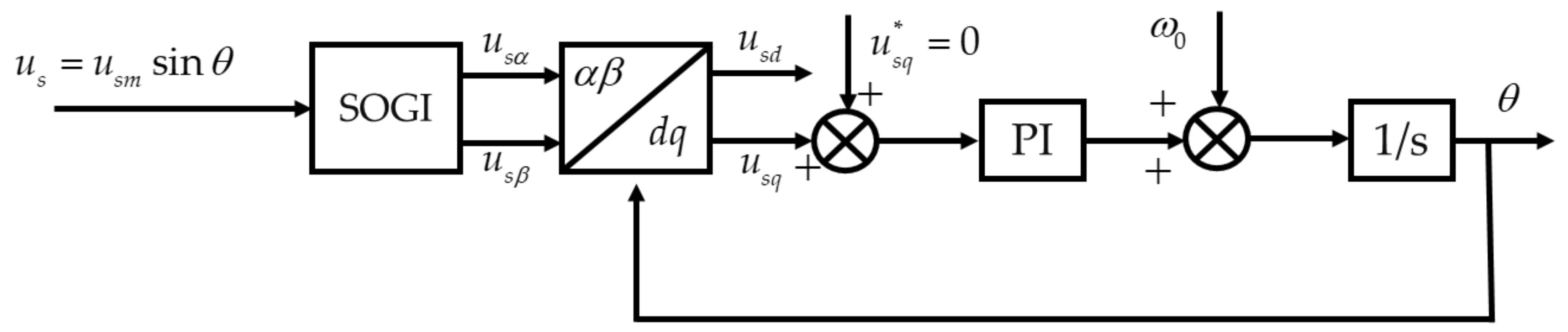
3.4. Implementation Scheme of Phase-Locked Loop

In order to achieve unity power factor control, the phase of the AC voltage needs to be obtained. The phase is obtained through a phase-locked loop (PLL). In Figure 4, u s q * is the reference value of the reactive component. In order to achieve unity power factor, u s q * should be set to 0.

3.5. The Control System of the Proposed MPCC

Figure 5a is the control block diagram of the system. The output of the PI voltage controller is multiplied by the sine value of the phase of the input voltage to obtain the current reference value i r e f . The function of the notch filter is to filter out the secondary ripple in the DC-link voltage. Then, the sampling values of input voltage and current and the reference value of input current are substituted into the inner current controller, and the PWM control signals are output by the inner current controller.
Figure 5b is the control flow chart of the inner current controller. First, the sampling values of AC voltage and input current are substituted into Equation (15) to calculate t o n k + 1 . Then t o n k + 1 is substituted into Equation (11) to calculate i s k + 2 , and then i r e f and i s k + 2 are substituted into Equation (13) to calculate the value of cost function. By comparing the value of the cost function under the two effective vectors, the effective vector corresponding to the smaller value of the cost function and its optimal action time are selected. Finally, the on-time of each switch is calculated and output according to Table 3.

4. Dead-Time Compensation

Figure 6 is the comparison of the switch states before and after adding the dead-time. T d is the dead-time, and the labels 1–4 in the figure respectively represent the conduction periods of switches S 1 ~ S 4 before adding the dead-time.
In the switch state after adding dead-time in Figure 6, when the effective vector is (1,0,0,1), the regions of label 1 and label 4 in the figure originally belong to the effective vector’s action time, and label 2 and label 3 originally belong to the zero vector’s action time; when the effective vector is (0,1,1,0), the regions of label 1 and label 4 in the figure originally belong to the zero vector’s action time, and label 2 and label 3 originally belong to the effective vector’s action time. Therefore, after adding dead-time, the effective vector and zero vector’s action time are reduced by 2 T d respectively.
It can be seen from Figure 6 that there are four kinds of switching vectors during the dead-time, which are (1,0,0,0), (0,1,0,0), (0,0,1,0), and (0,0,0,1). For the four switching vectors, only one switch is turned on, so the anti-parallel diode of the other switch must be turned on and freewheel. Combined with the current direction, the current paths under these four switching vectors can be determined, as shown in Figure 7 and Figure 8. Figure 7 and Figure 8 are the cases when the input current is greater than 0 and less than 0, respectively.
According to Figure 7 and Figure 8, we can get the values of u a b under these four switching vectors, as shown in Table 4.
From Figure 6 we can know that when the effective vector is (1,0,0,1), there are two kinds of switching vectors in the dead-time, (1,0,0,0) and (0,0,0,1), and both of which have an action time of 2 T d . According to Table 4, when i s > 0 , u a b under these two switching vectors is equal to u d c , which is equivalent to the actual action time of the effective vector is ( t o n 2 T d + 4 T d ) , that is, ( t o n + 2 T d ) , and the remaining time is the zero vector‘s action time. Then the current prediction equation should be revised as
i s k + 1 = i s k + t o n k 2 T d + 4 T d L u s k u d c + T s t o n k 2 T d L u s k = i s k + T s L u s k 2 T d L u d c t o n k L u d c
When the effective vector is (1,0,0,1) and i s < 0 , it can be seen from Table 4 that u a b is equal to 0, which is equivalent to the actual action time of the zero vector is ( T s t o n 2 T d + 4 T d ) , that is, ( T s t o n + 2 T d ) . Then, the current prediction equation should be revised as
i s k + 1 = i s k + t o n k 2 T d L u s k u d c + T s t o n k 2 T d + 4 T d L u s k = i s k + T s L u s k + 2 T d L u d c t o n k L u d c
When the effective vector is (0,1,1,0), the two switching vectors in the dead-time are (0,1,0,0) and (0,0,1,0), respectively. Similarly, it can be concluded that the current prediction equation should be revised as
When i s > 0 ,
i s k + 1 = i s k + T s L u s k 2 T d L u d c + t o n k L u d c
When i s < 0 ,
i s k + 1 = i s k + T s L u s k + 2 T d L u d c + t o n k L u d c
Since the effective vector (1,0,0,1) corresponds to S a b = 1 and the effective vector (0,1,1,0) corresponds to S a b = 1 , the current prediction equation can be summarized as Equations (20) and (21) according to (16)~(19).
When i s > 0 ,
i s k + 1 = i s k + T s L u s k 2 T d L u d c t o n k L S a b k u d c
When i s < 0 ,
i s k + 1 = i s k + T s L u s k + 2 T d L u d c t o n k L S a b k u d c
Then in order to reduce the error caused by the control delay, it is necessary to calculate the current prediction value at instant k + 2. Due to the high sampling frequency, we can assume that the current direction remains unchanged in two adjacent sampling periods. Then, we can get
When i s > 0 ,
i s k + 2   i s k + 1 = T s L u s k + 1 2 T d L u d c t o n k + 1 L S a b k + 1 u d c
When i s < 0 ,
i s k + 2   i s k + 1 = T s L u s k + 1 + 2 T d L u d c t o n k + 1 L S a b k + 1 u d c
Substituting Equations (9) and (10) into (22) and (23), the final current prediction equation can be expressed as
When i s > 0 ,
i s k + 2 = i s k + 2 T s L 2 u s k u s k 1 4 T d L u d c 2 t o n k + 1 L S a b k + 1 u d c
When i s < 0 ,
i s k + 2 = i s k + 2 T s L 2 u s k u s k 1 + 4 T d L u d c 2 t o n k + 1 L S a b k + 1 u d c
Then substituting Equations (24) and (25) into (14) to derive the cost function, and finally get the optimal action time of the effective vector as:
When i s > 0 ,
t o n k + 1 = L i s k i r e f + 2 T s L 2 u s k u s k 1 4 T d L u d c 2 S a b k + 1 u d c
When i s < 0 ,
t o n k + 1 = L i s k i r e f + 2 T s L 2 u s k u s k 1 + 4 T d L u d c 2 S a b k + 1 u d c
When t o n k + 1 is calculated to be greater than T s , let it be equal to T s ; when t o n k + 1 is calculated to be less than 0, let it be equal to 0.
Figure 9 is the flow chart of the inner current controller with dead-time compensation. The difference with Figure 5b is that there is an extra process of judging the polarity of the current, and the corresponding current prediction equation is selected according to the polarity of the current.

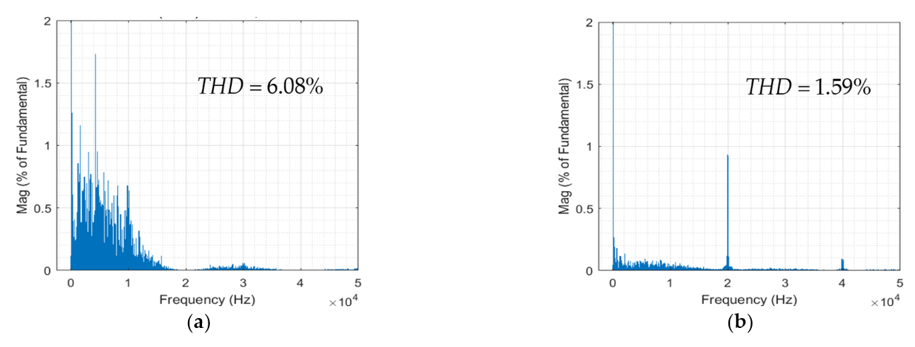
5. Simulation Results

The proposed MPCC scheme was simulated in MATLAB/Simulink. The peak value of the AC voltage was set to 60 V, filter inductance to 10 mH, reference value of DC-link voltage to 120 V, load resistance to 150 Ω, and sampling frequency to 20 kHz.
Figure 10 shows the current waveforms of the proposed MPCC and FCS-MPC without adding the dead-time, and Figure 11 shows the FFT analysis results of the current waveforms. The results show that the current of FCS-MPC contains a large number of low-order harmonics, the current harmonics of the proposed MPCC are mainly concentrated at the switching frequency and its multiples, and there are fewer low-order harmonics, which greatly reduces the current THD.
In order to make the influence of the dead-time more obvious, simulation was performed after adding the dead-time of 6 µs. Without dead-time compensation, the current waveform obtained is shown in Figure 12. It can be seen that the current waveform has been significantly distorted, and a relatively long clamping time occurs when the current crosses zero, and the current THD has increased to 3.28%.
The current waveform after adding dead-time compensation is shown in Figure 13. At this time, there is basically no clamping time when the current crosses zero, and the current THD is reduced to 1.94%, which is close to 1.59% when there is no dead-time, successfully suppressing the zero-current clamping effects and verifying the effectiveness of the algorithm.

6. Experimental Results

In order to verify the effectiveness of the proposed control system, a low-power experimental platform for single-phase PWM rectifier was built, as shown in Figure 14.
The power supply is provided by autotransformer in the experimental system. The power MOSFET of the main power circuit is C3M0120090D of CREE. Texas Instruments TMS320F28335 is chosen as the controller. Power factor (PF) was measured by power meter, PF9800.

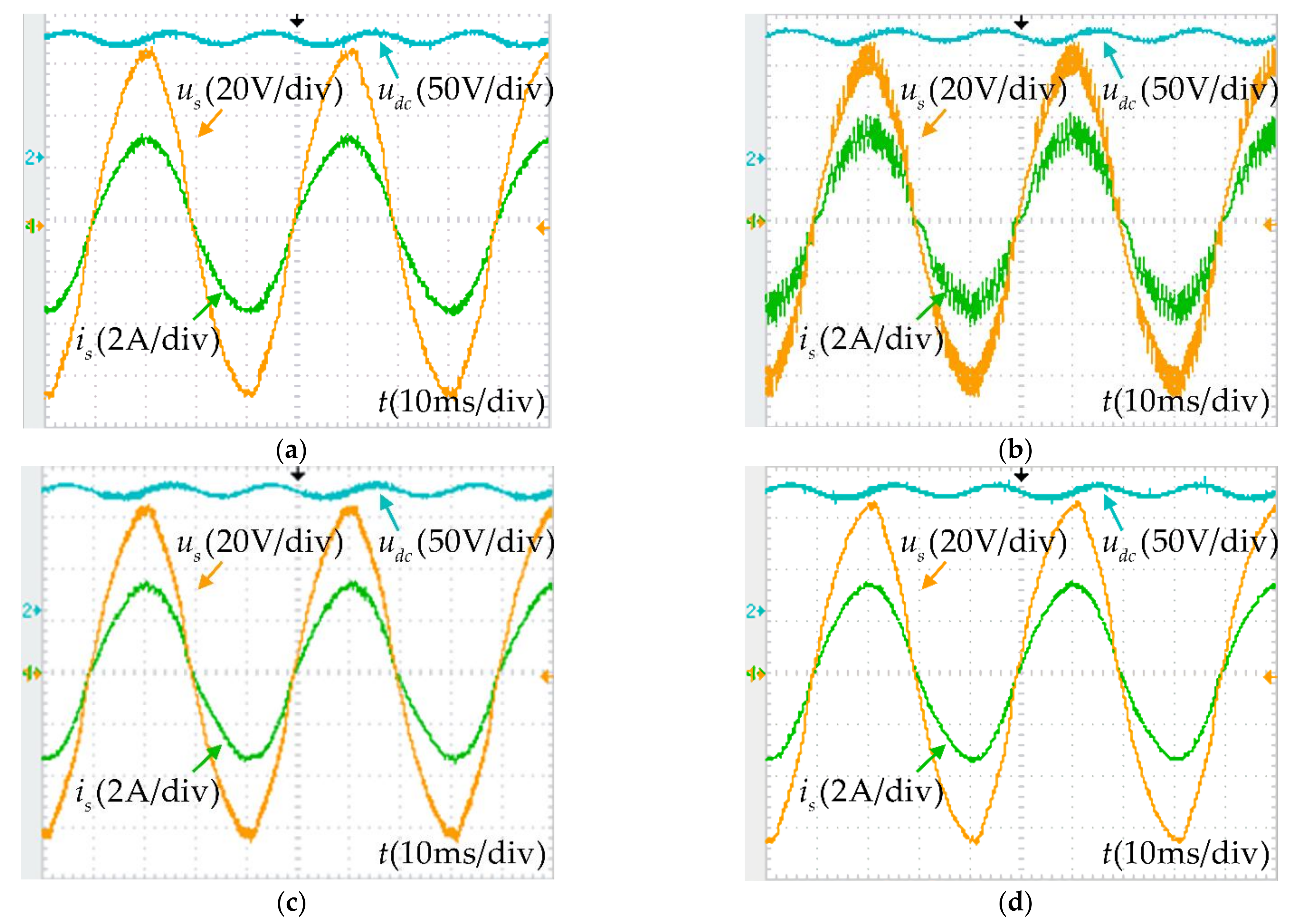
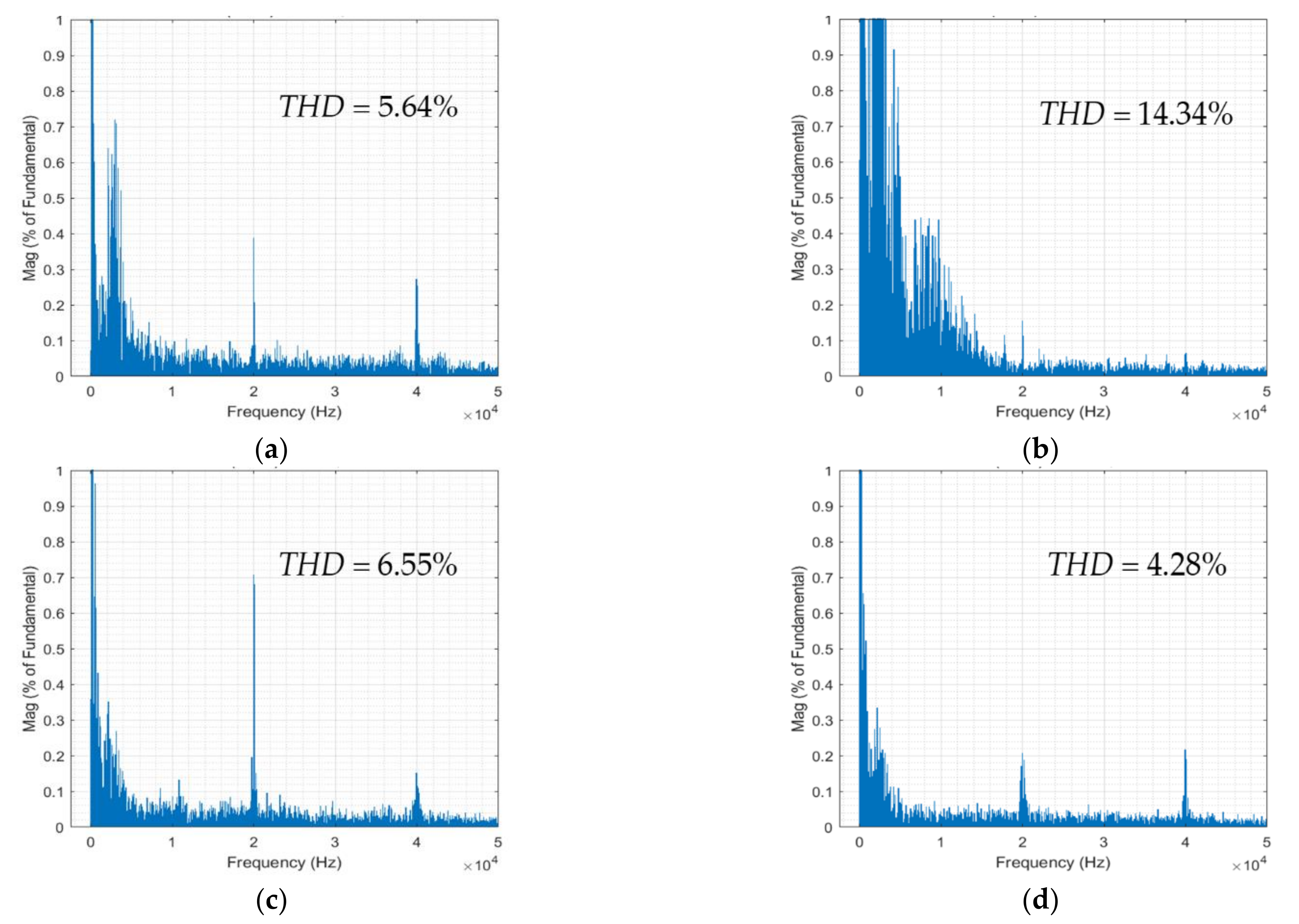
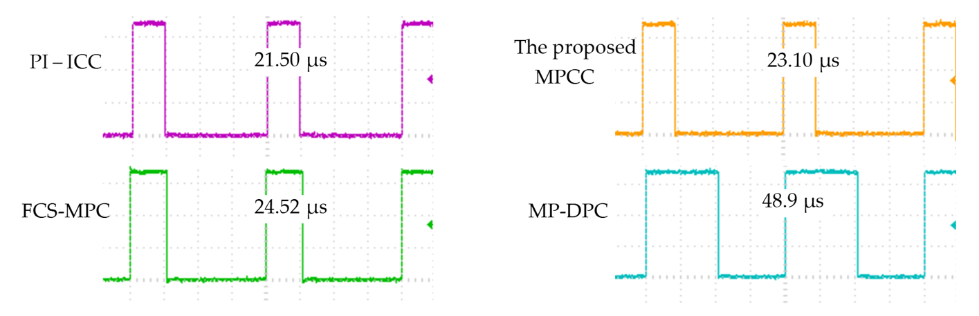
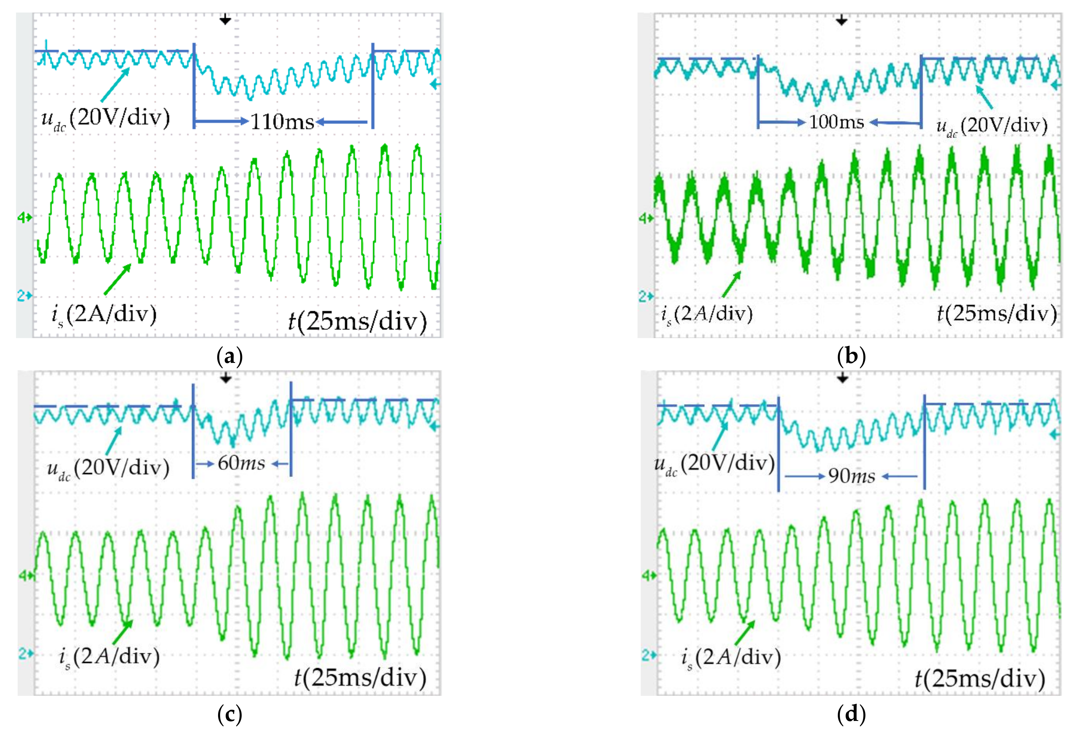
6.1. Performance Comparison with Other Algorithms

The experimental parameters are shown in Table 5. The experimental results of the proposed MPCC and FCS-MPC, PI-ICC and MP-DPC are compared and analyzed.
From the experimental waveforms in Figure 15, it can be seen that the four algorithms can make the input current sinusoidal, but it is also obvious that there are differences in the content of harmonic currents under different algorithms. Among them, the current waveform distortion of FCS-MPC scheme is the most serious. This is because the FCS-MPC scheme uses only one switching vector in a sampling period, and the switching frequency is not fixed and low. From the results of the fast Fourier transform (FFT) analysis, as shown in Figure 16, the current THD of FCS-MPC has reached 14.34%. PI-ICC, MP-DPC and the proposed MPCC can all make the switching frequency fixed. Among them, the current THD of the proposed MPCC is 4.28%, which is less than 5.64% of PI-ICC and 6.55% of MP-DPC. Therefore, in these four algorithms, the proposed MPCC can achieve the lowest current THD and remain the switching frequency fixed.
Figure 17 shows the comparison of the execution time of these four algorithms. The algorithm is calculated in the interrupt program of the digital signal processor (DSP). Configuring a General-purpose input/output (GPIO) port of the DSP as an output port, set it to 1 at the beginning of the program, clear it at the end of the program, and set the interrupt cycle to 100 µs. Then, the time when the output of the GPIO port is high is the execution time. The PI-ICC scheme’s inner controller adopts PI controller, which only requires one calculation, so the execution time is the shortest; the proposed MPCC needs to perform two cycles to calculate the predicted current value, and its execution time is slightly longer than the PI-ICC scheme; FCS-MPC needs to perform at least three cycles to calculate the predicted current value, so its execution time is longer than the proposed MPCC; compared with the proposed MPCC, MP-DPC requires additional coordinate translation and coordinate transformation of AC voltage and current to calculate active and reactive power, so its execution time is the longest, which is close to 2.1 times the execution time of the proposed MPCC.
In order to compare the dynamic response performance of the DC-link voltage of the four algorithms, a load mutation experiment was carried out, the load resistance was stepped from 250 Ω to 150 Ω. The experimental waveforms are shown in Figure 18. The settling time of the DC-link voltage is determined by the PI voltage controller and the inner current or power controller. This paper sets the same parameters for the PI voltage controller. From the results, the settling time of MP-DPC scheme is the shortest. This is because MP-DPC adopts an inner power controller, which adjusts the DC-link voltage directly by adjusting the output power. The other three algorithms adopt inner current controllers, which adjust the DC-link voltage by adjusting the input current, so the settling time is longer. Among the three algorithms adopting inner current controllers, PI-ICC has the longest settling time due to the integration loop’s hysteresis effect.
It can be seen from Table 6, Compared with PI-ICC scheme, the proposed MPCC has the following advantages: low current THD, fast dynamic response of DC-link voltage, and fewer parameters to be tuned due to its fewer PI controllers.
Compared with FCS-MPC, the proposed MPCC fixes the switching frequency, the value of current THD is significantly reduced.
Compared with MP-DPC, the proposed MPCC greatly reduces the current THD and greatly shortens the execution time. However, in terms of dynamic response performance of the DC-link voltage, the inner power controller is better than the inner current controller.

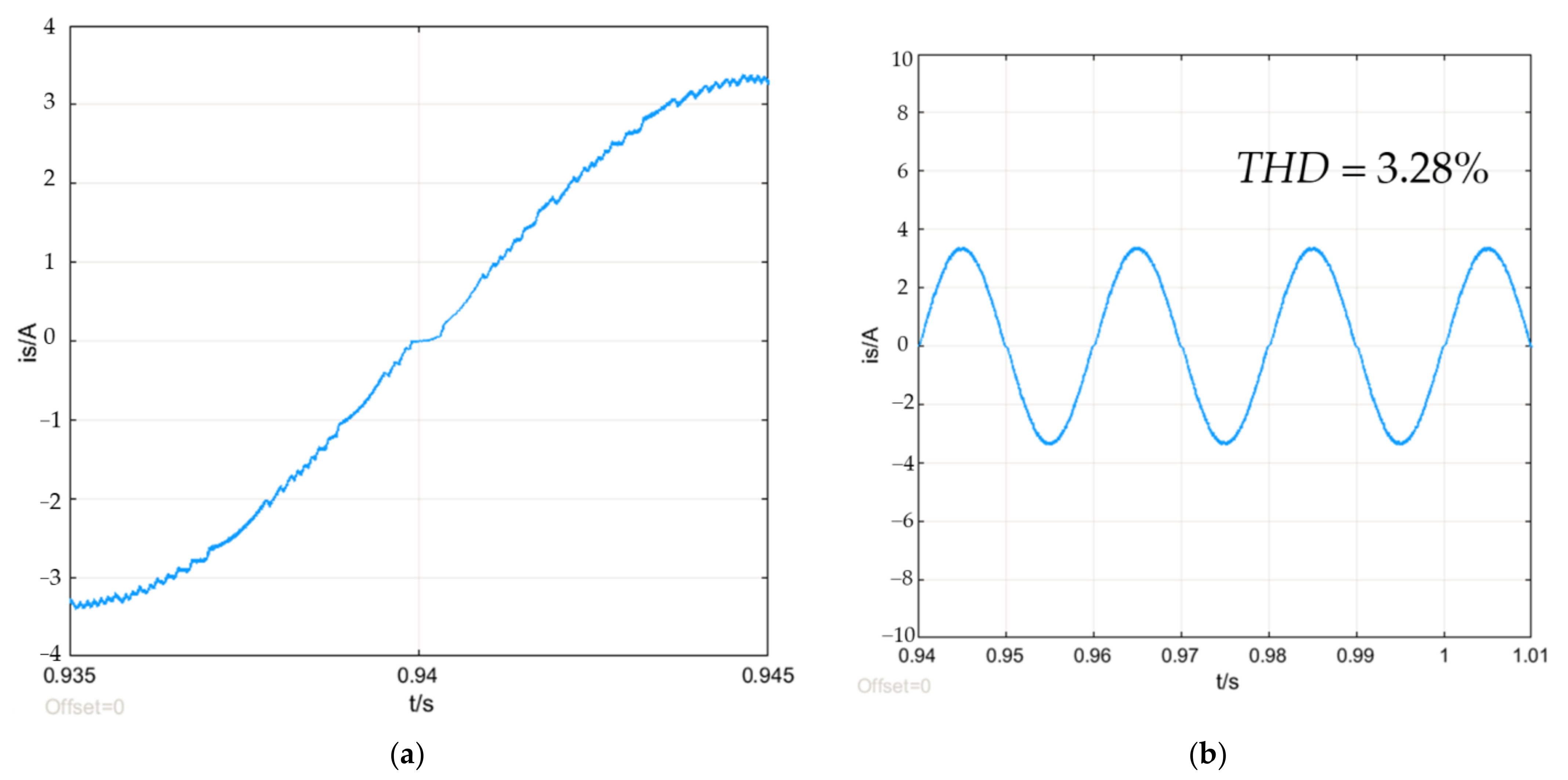
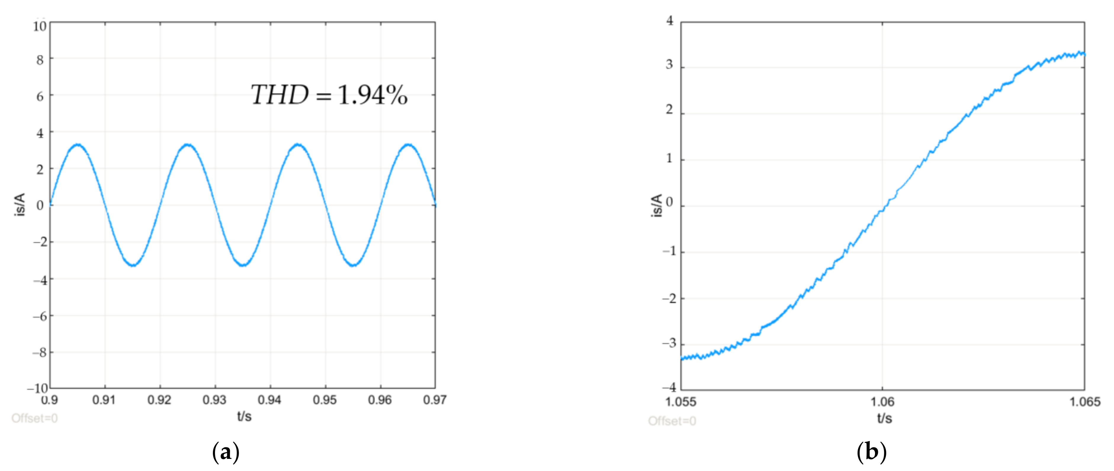
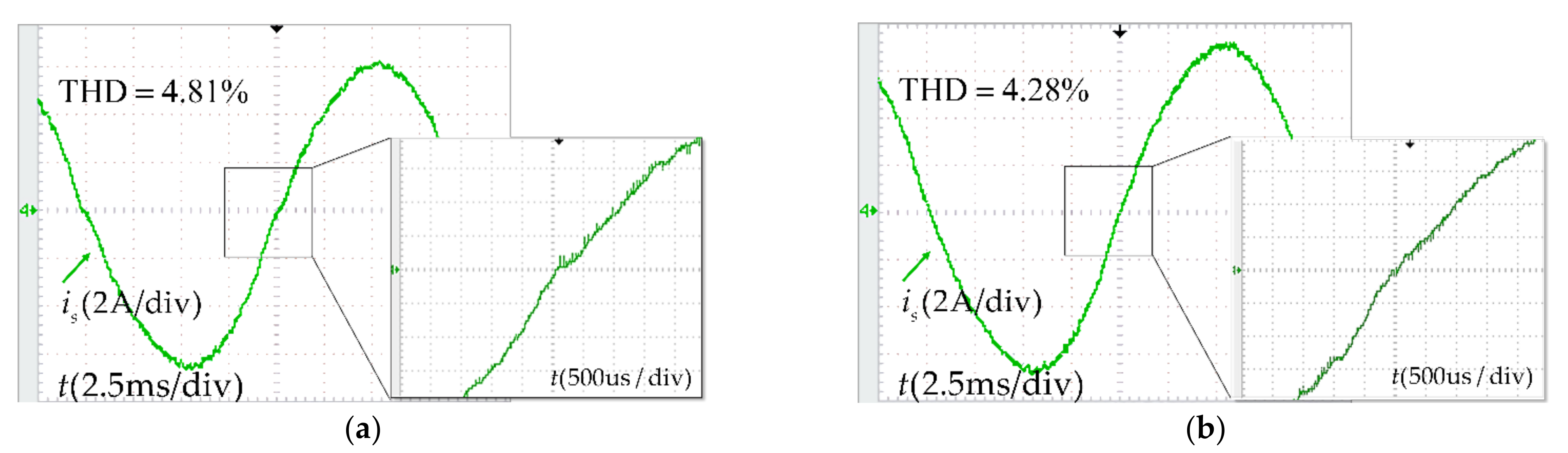
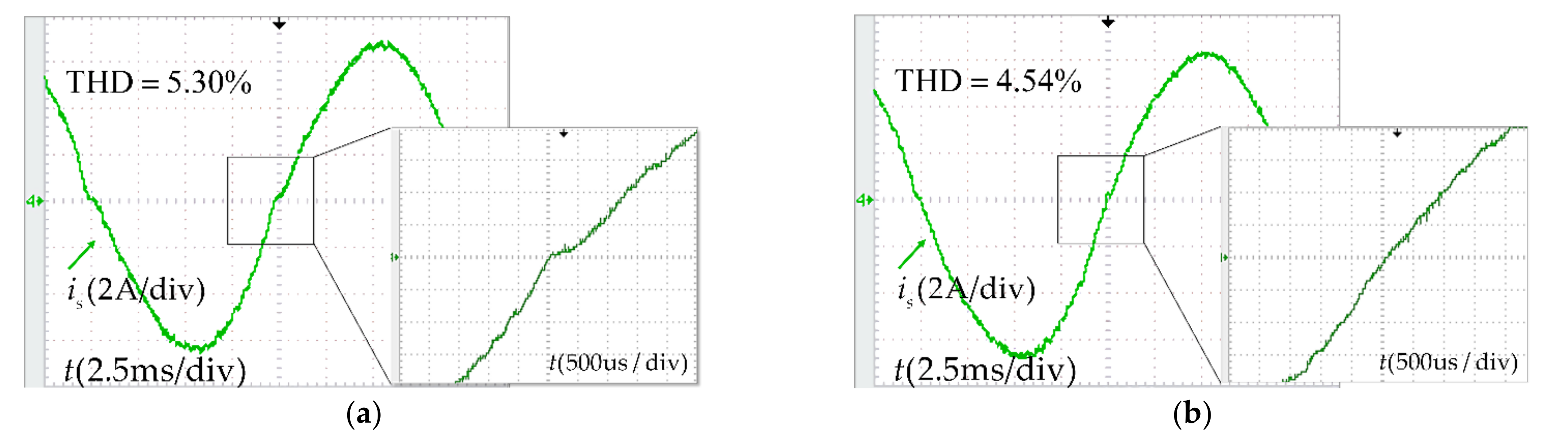
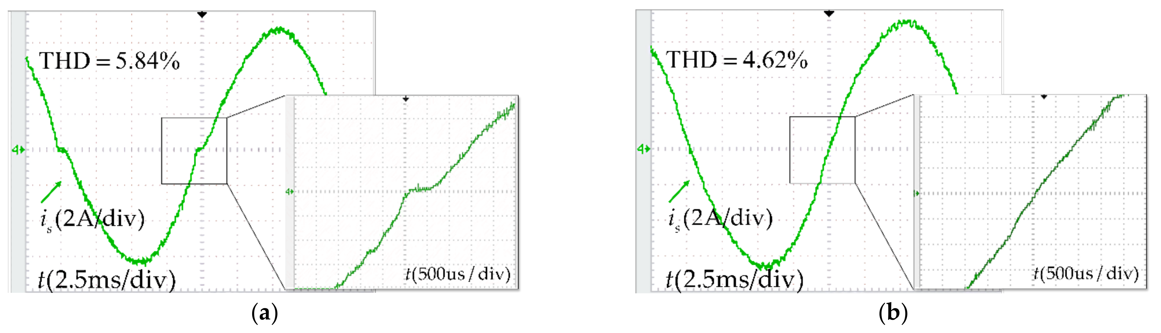
6.2. Experiment of Dead-Time Compensation

The experimental parameters are basically the same as Table 5. In order to compare the compensation effects under different dead-time, experiments with dead-time of 2 µs, 4 µs, and 6 µs were carried out. Figure 5b and Figure 9 are the control flow of the no compensation scheme and with compensation scheme, respectively. The experimental waveforms are as follows.
According to Figure 19, Figure 20 and Figure 21, the experimental results can be summarized in Table 7, and the relationships between the dead-time and THD, PF or clamping time is drawn according to Table 7 as shown in Figure 22.
Experimental results show that without dead-time compensation, as the dead time increases, the zero-current clamping effects become more obvious. When the dead-time increases from 2 µs to 6 µs, the clamping time increases from 200 µs to 500 µs, the current THD increases from 4.81% to 5.84%. After adding the dead-time compensation, the current waveform has no obvious distortion under different dead-time, basically no clamping time, the current THD is kept at a low level. PF was measured online by a power meter. The accuracy of the power meter is ± (0.4% reading + 0.1% range + 1 word), and the range is (−1.000~1.000). From the results, within the error range, under the dead-time of 2 µs to 6µs, both uncompensated and compensated schemes can achieve high power factor.

7. Conclusions

In order to reduce the harmonic current of the single-phase PWM rectifier, based on the model predictive control algorithm, this paper proposes an MPCC scheme with fixed switching frequency and dead-time compensation. The principle of fixed switching frequency control is analyzed, and the current prediction model is established; the influence of the dead-time on the switching vector is discussed and the prediction model is revised.
From the simulation results, FCS-MPC has a large number of low-order harmonics in the current because the switching frequency is not fixed. In the current obtained by the proposed MPCC, the harmonic current at the switching frequency is the main component, and the current THD is greatly reduced. The simulation results also show that the addition of the dead-time will bring about zero-current clamping effects and increase the value of THD. The compensation algorithm proposed in this paper can effectively suppress the dead-time effects and reduce the current THD.
The experimental results of the proposed MPCC were compared with those of FCS-MPC, MP-DPC and PI-ICC. The results show that the proposed MPCC can achieve the lowest current THD. In addition, the proposed MPCC also has these advantages: unit power factor, shorter execution time compared with MP-DPC, fewer adjusted parameters and shorter settling time of DC-link voltage compared with PI-ICC. Then, the dead-time compensation experiment was carried out. The experimental results show that the dead-time compensation algorithm can effectively suppress the zero-current clamping effects, there is basically no clamping time, and the current THD can be kept at a low level under different dead-time.
This algorithm helps to give full play to the advantages of MPC and enhance the practical engineering application of MPC algorithm. In addition, research on sensitivity of inductance parameters is also under way.

Author Contributions

All authors contributed to this work by collaboration. Conceptualization, L.K. and J.Z.; methodology, J.Z.; validation, J.Z., H.Z.; formal analysis, J.Z.; investigation, J.Z.; resources, L.K.; writing-original draft preparation, J.Z.; writing—review and editing, H.Z., Z.Z., X.D.; project administration, L.K.; funding acquisition, L.K. All authors have read and agreed to the published version of the manuscript.

Funding

This work was supported by Key Area R&D Program of Guangdong Province (2019B090911001).

Acknowledgments

I would like to be very grateful to my mentor Longyun Kang, who helped me a lot in my experiment and writing process.

Conflicts of Interest

The authors declare no conflict of interest.

References

  1. Krein, P.T.; Balog, R.S.; Mirjafari, M. Minimum Energy and Capacitance Requirements for Single-Phase Inverters and Rectifiers Using a Ripple Port. IEEE Trans. Power Electron. 2012, 27, 4690–4698. [Google Scholar] [CrossRef]
  2. Youssef, A.B.; El Khil, S.K.; Slama-Belkhodja, I. State Observer-Based Sensor Fault Detection and Isolation, and Fault Tolerant Control of a Single-Phase PWM Rectifier for Electric Railway Traction. IEEE Trans. Power Electron. 2013, 28, 5842–5853. [Google Scholar] [CrossRef]
  3. Komurcugil, H.; Altin, N.; Ozdemir, S.; Sefa, I. An Extended Lyapunov-Function-Based Control Strategy for Single-Phase UPS Inverters. IEEE Trans. Power Electron. 2015, 30, 3976–3983. [Google Scholar] [CrossRef]
  4. Dixon, J.W.; Ooi, B. Indirect Current Control of a Unity Power Factor Sinusoidal Current Boost Type Three-Phase Rectifier. IEEE Trans. Ind. Electron. 1988, 35, 508–515. [Google Scholar] [CrossRef]
  5. Albanna, A.Z.; Hatziadoniu, C.J. Harmonic Modeling of Hysteresis Inverters in Frequency Domain. IEEE Trans. Power Electron. 2010, 25, 1110–1114. [Google Scholar] [CrossRef]
  6. Viswadev, R.; Mudlapur, A.; Ramana, V.V.; Venkatesaperumal, B.; Mishra, S. A Novel AC Current Sensorless Hysteresis Control for Grid-Tie Inverters. IEEE Trans Circuits Syst. II Express Briefs 2020, 67, 2577–2581. [Google Scholar] [CrossRef]
  7. Brenna, M.; Foiadelli, F.; Zaninelli, D. New Stability Analysis for Tuning PI Controller of Power Converters in Railway Application. IEEE Trans. Ind. Electron. 2011, 58, 533–543. [Google Scholar] [CrossRef]
  8. Song, H.; Keil, R.; Mutschler, P.; van der Weem, J.; Nam, K. Advanced Control Scheme for a Single-Phase PWM Rectifier in Traction Applications. In Proceedings of the 38th IAS Annual Meeting on Conference Record of the Industry Applications Conference, Salt Lake City, UT, USA, 12–16 October 2003; pp. 1558–1565. [Google Scholar]
  9. Husev, O.; Roncero-Clemente, C.; Makovenko, E.; Pimentel, S.P.; Vinnikov, D.; Martins, J. Optimization and Implementation of the Proportional-Resonant Controller for Grid-Connected Inverter with Significant Computation Delay. IEEE Trans. Ind. Electron. 2020, 67, 1201–1211. [Google Scholar] [CrossRef]
  10. Mateev, V.; Ralchev, M.; Marinova, I. Current Sensor Accuracy Enhancement by Harmonic Spectrum Analysis. In Proceedings of the 13th International Conference on Sensing Technology (ICST), Sydney, Australia, 2–4 December 2019; pp. 1–4. [Google Scholar]
  11. Berg, M.; Roinila, T. Dynamic Effect of Input-Voltage Feedforward in Three-Phase Grid-Forming Inverters. Energies 2020, 13, 2923. [Google Scholar] [CrossRef]
  12. Kwak, S.; Moon, U.; Park, J. Predictive-Control-Based Direct Power Control with an Adaptive Parameter Identification Technique for Improved AFE Performance. IEEE Trans. Power Electron. 2014, 29, 6178–6187. [Google Scholar] [CrossRef]
  13. Panten, N.; Hoffmann, N.; Fuchs, F.W. Finite Control Set Model Predictive Current Control for Grid-Connected Voltage-Source Converters with LCL Filters: A Study Based on Different State Feedbacks. IEEE Trans. Power Electron. 2016, 31, 5189–5200. [Google Scholar] [CrossRef]
  14. Ahmed, A.A.; Koh, B.K.; Lee, Y.I. A Comparison of Finite Control Set and Continuous Control Set Model Predictive Control Schemes for Speed Control of Induction Motors. IEEE Trans. Ind. Inform. 2018, 14, 1334–1346. [Google Scholar] [CrossRef]
  15. Wang, W.; Fan, Y.; Chen, S.; Zhang, Q. Finite Control Set Model Predictive Current Control of a Five-Phase PMSM with Virtual Voltage Vectors and Adaptive Control Set. CES Trans. Electr. Mach. Syst. 2018, 2, 136–141. [Google Scholar] [CrossRef]
  16. Zhang, Y.; Peng, Y.; Yang, H. Performance Improvement of Two-Vectors-Based Model Predictive Control of PWM Rectifier. IEEE Trans. Power Electron. 2016, 31, 6016–6030. [Google Scholar] [CrossRef]
  17. Nikhil, P.; Sonam, K.; Monika, M.; Wagh, S. Finite Control Set Model Predictive Control for Two Level Inverter with Fixed Switching Frequency. In Proceedings of the 2018 SICE International Symposium on Control Systems (SICE ISCS), Tokyo, Japan, 9–11 March 2018; pp. 74–81. [Google Scholar]
  18. Malinowski, M.; Jasinski, M.; Kazmierkowski, M.P. Simple Direct Power Control of Three-Phase PWM Rectifier Using Space-Vector Modulation (DPC-SVM). IEEE Trans. Ind. Electron. 2004, 51, 447–454. [Google Scholar] [CrossRef]
  19. Bouafia, A.; Gaubert, J.P.; Krim, F. Predictive Direct Power Control of Three-Phase Pulsewidth Modulation (PWM) Rectifier Using Space-Vector Modulation (SVM). IEEE Trans. Power Electron. 2010, 25, 228–236. [Google Scholar] [CrossRef]
  20. Tarisciotti, L.; Zanchetta, P.; Watson, A.; Clare, J.C.; Degano, M.; Bifaretti, S. Modulated Model Predictive Control for a Three-Phase Active Rectifier. IEEE Trans. Ind. Appl. 2015, 51, 1610–1620. [Google Scholar] [CrossRef]
  21. Antoniewicz, P.; Kazmierkowski, M.P. Virtual-Flux-Based Predictive Direct Power Control of AC/DC Converters with Online Inductance Estimation. IEEE Trans. Ind. Electron. 2008, 55, 4381–4390. [Google Scholar] [CrossRef]
  22. Hu, B.; Kang, L.; Liu, J.; Zeng, J.; Wang, S.; Zhang, Z. Model Predictive Direct Power Control with Fixed Switching Frequency and Computational Amount Reduction. IEEE J. Emerg. Sel. Top. Power Electron. 2019, 7, 956–966. [Google Scholar] [CrossRef]
  23. Ramirez, R.O.; Espinoza, J.R.; Villarroel, F.; Maurelia, E.; Reyes, M.E. A Novel Hybrid Finite Control Set Model Predictive Control Scheme with Reduced Switching. IEEE Trans. Ind. Electron 2014, 61, 5912–5920. [Google Scholar] [CrossRef]
  24. Kang, L.; Cheng, J.; Hu, B.; Luo, X.; Zhang, J. A Simplified Optimal-Switching-Sequence MPC with Finite-Control-Set Moving Horizon Optimization for Grid-Connected Inverter. Electronics 2019, 8, 457. [Google Scholar] [CrossRef] [Green Version]
  25. Liu, J.; Cheng, S.; Liu, Y.; Shen, A. FCS-MPC for a Single-Phase Two-Stage Grid-Connected PV Inverter. IET Power Electron. 2019, 12, 915–922. [Google Scholar] [CrossRef]
  26. Azab, M. Performance of Model Predictive Control Approach for Single-Phase Distributed Energy Grid Integration with PQ Control. IET Energy Syst. Integr. 2019, 1, 121–132. [Google Scholar] [CrossRef]
  27. Yang, Y.; Wen, H.; Fan, M.; Xie, M.; Chen, R.; Wang, Y. A Constant Switching Frequency Model Predictive Control without Weighting Factors for T-Type Single-Phase Three-Level Inverters. IEEE Trans. Ind. Electron. 2019, 66, 5153–5164. [Google Scholar] [CrossRef]
  28. Song, W.; Deng, Z.; Wang, S.; Feng, X. A Simple Model Predictive Power Control Strategy for Single-Phase PWM Converters with Modulation Function Optimization. IEEE Trans. Power Electron. 2016, 31, 5279–5289. [Google Scholar] [CrossRef]
  29. Herran, M.A.; Fischer, J.R.; Gonzalez, S.A.; Judewicz, M.G.; Carrica, D.O. Adaptive Dead-Time Compensation for Grid-Connected PWM Inverters of Single-Stage PV Systems. IEEE Trans. Power Electron. 2013, 28, 2816–2825. [Google Scholar] [CrossRef]
  30. Mora, A.; Juliet, J.; Santander, A.; Lezana, P. Dead-Time and Semiconductor Voltage Drop Compensation for Cascaded H-Bridge Converters. IEEE Trans. Ind. Electron. 2016, 63, 7833–7842. [Google Scholar] [CrossRef]
  31. Liu, G.; Wang, D.; Jin, Y.; Wang, M.; Zhang, P. Current-Detection-Independent Dead-Time Compensation Method Based on Terminal Voltage A/D Conversion for PWM VSI. IEEE Trans. Ind. Electron. 2017, 64, 7689–7699. [Google Scholar] [CrossRef]
  32. Kim, E.; Seong, U.; Lee, J.; Hwang, S. Compensation of Dead Time Effects in Grid-Tied Single-Phase Inverter Using SOGI. In Proceedings of the IEEE Applied Power Electronics Conference and Exposition (APEC), Tampa, FL, USA, 26–30 March 2017; pp. 2633–2637. [Google Scholar]
  33. Li, X.; Akin, B.; Rajashekara, K. Vector Based Dead-Time Compensation for Three-Level T-type Converters. IEEE Trans. Ind. Appl. 2016, 52, 1597–1607. [Google Scholar]
  34. Hu, B.; Kang, L.; Cheng, J.; Linghu, J.; Zhang, Z. Integrated Dead-Time Compensation and Elimination Approach for Model Predictive Power Control with Fixed Switching Frequency. IET Power Electron. 2019, 12, 1220–1228. [Google Scholar] [CrossRef]
  35. Lin, Y.; Lai, Y. Dead-Time Elimination of PWM-Controlled Inverter/Converter without Separate Power Sources for Current Polarity Detection Circuit. IEEE Trans. Ind. Electron. 2009, 56, 2121–2127. [Google Scholar]
  36. Chen, L.; Peng, F.Z. Dead-Time Elimination for Voltage Source Inverters. IEEE Trans. Power Electron. 2008, 23, 574–580. [Google Scholar] [CrossRef]
Figure 1. The topology of a single-phase PWM rectifier.
Electronics 10 00426 g001
Figure 2. Possible switching vectors of FCS-MPC.
Electronics 10 00426 g002
Figure 3. Possible switching vector combinations of the proposed MPCC.
Electronics 10 00426 g003
Figure 4. The control structure of the PLL.
Electronics 10 00426 g004
Figure 5. The control system of the proposed MPCC. (a) Control block diagram of the system; (b) Control flow chart of the inner current controller.
Electronics 10 00426 g005
Figure 6. Comparison of switch states before and after adding dead-time.
Electronics 10 00426 g006
Figure 7. The current path during the dead-time when i s > 0 . (a) (1,0,0,0); (b) (0,1,0,0); (c) (0,0,1,0); (d) (0,0,0,1).
Electronics 10 00426 g007
Figure 8. The current path during the dead-time when i s < 0 . (a) (1,0,0,0); (b) (0,1,0,0); (c) (0,0,1,0); (d) (0,0,0,1).
Electronics 10 00426 g008
Figure 9. The flow chart of the inner current controller with dead-time compensation.
Electronics 10 00426 g009
Figure 10. Simulated current waveforms. (a) FCS-MPC; (b) the proposed MPCC.
Electronics 10 00426 g010
Figure 11. FFT analysis results of simulated current waveforms. (a) FCS-MPC; (b) the proposed MPCC.
Electronics 10 00426 g011
Figure 12. The simulated current waveform when the dead-time is 6us and there is no dead-time compensation. (a) The full cycle waveform of the current; (b) The waveform when the current crosses zero.
Electronics 10 00426 g012
Figure 13. The simulated current waveform when the dead-time is 6 µs and there is dead-time compensation. (a) The full cycle waveform of the current; (b) The waveform when the current crosses zero.
Electronics 10 00426 g013
Figure 14. The photo of the experimental platform.
Electronics 10 00426 g014
Figure 15. Experimental waveforms of AC voltage, input current, and DC-link voltage. (a) PI-ICC; (b) FCS-MPC; (c) MP-DPC; (d) the proposed MPCC.
Electronics 10 00426 g015
Figure 16. FFT analysis of the input current. (a) PI-ICC; (b) FCS-MPC; (c) MP-DPC; (d) the proposed MPCC.
Electronics 10 00426 g016
Figure 17. The execution time of these four algorithms.
Electronics 10 00426 g017
Figure 18. Experimental waveforms of the dynamic response of DC-link voltage. (a) PI-ICC; (b) FCS-MPC; (c) MP-DPC; (d) the proposed MPCC.
Electronics 10 00426 g018
Figure 19. The current waveform when the dead time is 2 µs. (a) No compensation (b) With compensation.
Electronics 10 00426 g019
Figure 20. The current waveform when the dead time is 4 µs. (a) No compensation (b) With compensation.
Electronics 10 00426 g020
Figure 21. The current waveform when the dead time is 6 µs. (a) No compensation (b) With compensation.
Electronics 10 00426 g021
Figure 22. Graph of the relationship between dead time and: (a) Clamping time; (b) THD; (c) PF.
Electronics 10 00426 g022
Table 1. Switching states table of single-phase PWM rectifiers.
S 1 S 2 S 3 S 4 u a b
1001 u d c
10100
0110 u d c
01010
Table 2. The conduction time of each switch under FCS-MPC.
Vectors(1,0,0,1)(0,1,1,0)(1,0,1,0)(0,1,0,1)
Switches
S 1 T s 0 T s 0
S 2 0 T s 0 T s
S 3 0 T s T s 0
S 4 T s 00 T s
Table 3. The conduction time of each switch under the proposed MPCC.
Combinations(1,0,0,1)
(1,0,1,0), (0,1,0,1)
(0,1,0,1)
(1,0,1,0), (0,1,0,1)
Switches
S 1 ( T s + t o n ) / 2 ( T s t o n ) / 2
S 2 ( T s t o n ) / 2 ( T s + t o n ) / 2
S 3 ( T s t o n ) / 2 ( T s + t o n ) / 2
S 4 ( T s + t o n ) / 2 ( T s t o n ) / 2
Table 4. The value of u a b in the dead-time.
(1,0,0,0)(0,1,0,0)(0,0,1,0)(0,0,0,1)
i s > 0 u a b = u d c u a b = 0 u a b = 0 u a b = u d c
i s < 0 u a b = 0 u a b = u d c u a b = u d c u a b = 0
Table 5. Parameters of the experimental system.
System ParametersSymbolValue
Filter inductanceL10 mH
DC-link capacitorC220 µF
DC-link voltage u d c 120 V
AC Voltage peak u s 60 V
Load resistance R L 150 Ω
Sampling frequency f s 20 kHz
Dead-time T d 2 µs
Table 6. Performances comparison of these four algorithms.
PerformancePI-ICCFCS-MPCMP-DPCThe Proposed MPCC
THD5.64%14.34%6.55%4.28%
Execution time21.50 µs24.52 µs48.9 µs23.10 µs
Settling time of DC voltage110 ms100 ms60 ms90 ms
PI controller number2111
Inner controllercurrentcurrentpowercurrent
Table 7. Results of the dead-time compensation experiment.
Dead-Time2 µs4 µs6 µs
Performance
Is There Compensation (yes or no)noyesnoyesnoyes
Clamping time200 µsnone300 µsnone500 µsnone
THD4.81%4.28%5.30%4.54%5.84%4.62%
PF1.0001.0001.0001.0000.9911.000
Publisher’s Note: MDPI stays neutral with regard to jurisdictional claims in published maps and institutional affiliations.

