Power Consumption Profiling of a Lightweight Development Board: Sensing with the INA219 and Teensy 4.0 Microcontroller

Abstract

At the heart of most technological advancements is a network of processors executing code and consuming energy. Understanding those systems’ energy consumption profiles provides optimisation possibilities and thus contributes to strategies for reducing energy consumption in general. This paper assesses the power consumption characteristics of a highly competitive low cost, small form factor development board (the Raspberry Pi4 model B), powered with the minimal load associated with its bare-metal configuration and the related impact on baseline power consumption. We also consider the load associated with an out-of-box operating system, running at several underclocking frequency scaling levels and the associated impact on baseline power consumption. Our experimental set-up consists of integrating an INA219 high-side current sense amplifier for the capturing of power, current, and voltage measurements; and a Teensy 4.0 microcontroller for sampling. Overall, our results indicate statistically significant differences in overall power consumption distribution characteristics across all models. Our results also indicate the presence of three distinct power phase envelopes and statistically significant differences in mean and median power measurements between the different underclocking frequency test cases and the bare-metal cases. Our results also indicate that power consumption is an increasing monotonic function across test scenarios. Finally, our results have also shown that isolating power consumption composite distributions increases model predictability from 67% to 97%.

1. Introduction

In today’s global society, the challenges faced in climate change have been at the forefront of discussion for several decades and are now even more prevalent, and have included a focus on societal energy consumption. This discussion becomes even more challenging considering the continuous increasing integration of technology and the development of solutions for the automation of most everyday tasks, and the dependence on these solutions by society. Specifically, the prevalence and ubiquitous nature of embedded devices, for example; those embedded within and across a wide range of systems/appliances, including consumer and home appliances such as microwave ovens, dishwashers, cookers, fridge freezers, home heating systems; consumer electronics such as mobile phones, digital cameras, desktop printers; medical applications; automotive systems such as collision avoidance systems, braking system, fuel monitoring systems, and even window wiper speed, for example. All these devices are executing code and consuming ever-increasing amounts of energy. In addition to this, the evolution of modern processors has continued to see growth in the number of transistors and components integrated into a single form factor, as well as an increase in CPU core frequencies; this increase in density has introduced a significant demand on power and energy by modern computer systems [1].

An additional paradigm shift is underway regarding sharing information between those previously mentioned devices and applications, which has been wrapped in what has been termed the Internet of Things (IoT). From a practical perspective, IoT aims to allow seamless communication between devices. In this regard, the previously mentioned list of devices and applications can now be augmented to include electronic or electrochemical sensors that monitor the environment in which we live. For example, temperature sensors, humidity sensors, pressure sensors, proximity sensors, infrared sensors, optical sensors, accelerometers, and gyroscopes, to mention a few [2].

These sensors can function in isolation or be embedded within more complex systems. They can be reliant on power by connecting to a mains supply or being self-reliant (to some degree) being powered off battery. They can have mission-critical functions to perform, and as such, running out of power can be a costly effect.

A device that has seen an explosion in its functional use has been the Raspberry Pi generation of single-board computer. Initially designed and developed as a teaching device for computer science teaching and as a cheap, accessible platform for similar use in developing countries, it has seen its use expand and proliferate into many different fields. Its specification and performance, allowing it to become a base-board for the connection of sensors and other devices.

At the heart of most of these technological advancements is a processor or network of processors, executing code and consuming energy. Understanding the energy consumption profiles of these would provide optimisation possibilities and reduce energy consumption in general. In order to assess the energy footprint of an application, irrespective of the architecture or system that the application will be executed on, ahead-of-time or just-in-time models of their execution are required. With that said, understanding the baseline characteristics of the devices on which applications will run is also of fundamental importance.

In this regard, this paper considers and models the baseline power consumption characteristics of a low cost, small form factor platform, the Raspberry Pi4 model B. We assess the power consumption characteristics of the Raspberry Pi executing at several clock frequency scaling levels, in particular; we underclock the platform to run at 600 MHz, 900 MHz, and 1200 MHz, in addition to its out-of-box, defined clocking frequency scaling level of 1500 MHz. We also strip the Raspberry Pi4 back to run as a bare-metal embedded device without an operating system and assess its power consumption characteristics. We undertake this analysis as a precursor to a proposed analysis of power, current, and voltage characteristics of interpreted applications to model the platform’s baseline characteristics.

This paper is structured as follows. In Section 2, we present an overview regarding the background of this work, defining the main research questions that this work considered relative to the associated literature. We conclude Section 2 with a review of the relevant literature. In Section 3, we present an overview of our experimental set-up, defining the hardware components and their integration for capturing power consumption measurements from the Raspberry Pi4 Model B. The results of this study are presented in Section 4. We present these results from a descriptive and inferential perspective, testing for the difference between observed power consumption magnitudes between a bare-metal mode of execution and that associated with an out-of-box Linux operating system. In the penultimate section, Section 5, we present an analysis of our results relative to the associated literature. Finally, Section 6 details our concluding remarks and the future direction of our research.

2. Background and Related Work

It seems well established that many factors influence overall system power consumption performance. Some of these factors, including CPU core frequencies, GPU characteristics, and memory having been considered in [3,4,5,6]. Other factors have also been identified, such as operating system build configuration options and kernel tintification [7]; and factors associated with the servicing of network traffic across Ethernet and WiFi [8,9]. Furthermore, many studies have considered the early generations of Raspberry Pi models and their power consumption characteristics, in isolation or as the core components within homogeneous and heterogeneous clusters, for example, [5,10,11]. In addition to this, the challenge of capturing accurate high precision and high-resolution power measurements without using expensive hardware has also been the topic of the research [12]. Addressing the challenge concerning the storage and transmission of sampled power consumption measurements using low-cost hardware has also been the focus of several works [12,13,14,15]. Attempting to address the deficit between the resolution that hardware-based performance monitors offer, through their associated performance counters, with the resolution associated with software-based performance monitoring was considered by Fieni, Rouvoy, and Seinturier in [16].

However, previous studies have failed to isolate from their results the effect of idle power and the broad distributional characteristics associated with those variables. More importantly, prior work has not considered power consumption distribution characteristics and their superposition from more well-behaved distributions. Furthermore, the Raspberry Pi 4 Model B, the latest single-board computer within the Raspberry Pi family, has seen little concentration concerning its power consumption characteristics.

Therefore, this study’s primary goal was to assess the idle power characteristics associated with the latest generation of Raspberry Pi, the Raspberry Pi4 Model B. More importantly, our goal was to assess the inner structure of the power consumption distributions associated with the Raspberry Pi4 Model B, stripped back and powered on bare-metal, as well as considering an out-of-box distribution of the Linux operating system. We aimed to model power consumption by considering sub-distributional structure alongside core CPU frequency effects, bare-metal effects, and the effects associated with an out-of-box operating system.

In this regard, this paper addresses several hypotheses:

• Is there evidence to suggest that average bare-metal idle power consumption is different across several system state configurations?
• Is there evidence to suggest that average idle power consumption is different across several processor clocking frequencies?
• Is there evidence to suggest that average idle power consumption is different between a bare-metal configuration and a configuration that includes a fully booted operating system?
• Is there evidence to support the claim that idle power consumption distributions are a superposition of finer, more conformal distributions?
• Is power consumption dependent on CPU core frequency, bare-metal configuration, operating system boot, and finer distribution characteristics?

Related Work

Specifically focusing on the Raspberry Pi3 generation of single board computers, the work of Paniego et al. in [17] considers architectural level performance counters in an attempt to identify a minimal set of counters that together explain a maximal proportion of the variance associated with power consumption on the Raspberry Pi3. Their models are linear regression-based with performance counter independent variables such as processor cycles, instructions completed, completed load/store instructions, branch prediction/misprediction, cache miss rates, and hardware interrupts, for example. Power consumption measurements are captured by integrating an INA219 current sense amplifier (Texas Instruments, Dallas, TX, USA), which is sampled using the Arduino UNO development board (Arduino, Somerville, MA, USA). Model building is dependent on the benchmark applications comprising the NAS [18], RODINIA [19], and LINPACK [20] benchmark suites. Performance counter observations are captured using the performance application programming interface (PAPI) [21]. Their results do not present any descriptive overview of the power consumption distributions associated with the benchmark applications analysed, although ranges of power consumption can be loosely estimated from inspection of inline bar charts. Their results would suggest that all applications analysed had power consumption magnitudes in the range of between 2 W and 3 W. Their main result is the communication of a linear regression model and the differences between real and model estimations.

Considering the effect of overclocking and underclocking on Raspberry Pi power consumption, the work of Astudillo-Salinas, Barrera-Salamea, Vázquez-Rodas, and Solano-Quinde in [3] focus on those effects associated with CPU, GPU, and SDRAM. Their experimental platform consisting of a Raspberry Pi B, one of the first Raspberry Pi boards to be manufactured, and a MAX471 sensor module (Maxim Integrated, San Jose, CA, USA) [22] for the capturing of power measurements. In addition to assessing underclocking, Astudillo-Salinas et al. assess the power consumption of the Raspberry Pi across multiple Linux operating system distributions, as well as the powering down of HDMI and Ethernet. Their results would suggest that irrespective of operating system, that idle power consumption of the Raspberry Pi B is approximately $1.22$ W. The powering down of HDMI results in a decrease in power consumption in the order of $8\%$, while disconnecting the Ethernet cable reduces power consumption by approximately $19\%$ relative to the idle power of $1.22$ W. On inspection of their findings, negligible effects were observed in respect to underclocking of SDRAM. Their results also suggest that CPU underclocking results in a maximum reduction in the order of $0.06$ W of of power irrespective of operating system. With respect to GPU power consumption, underclocking results in an average saving of approximately $0.08$ W.

Leading on from work by Paniego et al. in [17], Paniego et al. in [23] expand on their previous findings and consider the power consumption characteristics of a Raspberry Pi3${}^{+}$ generation of board. Their analysis details the differences in power consumption between the Raspberry Pi3 and Raspberry Pi3${}^{+}$, including the differences based on the number of threads executed. Their findings suggest increased power consumption trends for the Raspberry Pi3${}^{+}$ compared to the Raspberry Pi3 board. Furthermore, the effect from parallelism, as measured by the number of threads, shows an increase in power consumption levels progressing from single-threaded execution, dual threaded, to quad threaded. Their work also considers the effect on power consumption associated with processor underclocking. Although the assessment of the effect of parallelism is considered at the application level, the effect of implicit application instruction-level parallelism is not assessed. No detailed descriptive overview of power consumption distribution characteristics are provided, and in respect to regression model parameter estimates, no detailed overview of standard errors of regression coefficients and their significance can be found. Interestingly though, the work of Paniego et al. in both [17,23] suggest that architectural level performance counters, and the degree of inherent parallelism, are parameters that account for a proportion of the variation in power consumption levels of applications running on Raspberry Pi generation boards.

More recently; Paniego et al. in [24] build on their previous work communicated within [17,23], and consider alternative models to the typical multiple linear regression analysis. Their addition includes machine learning techniques such as support vector regression, Gaussian regression, and kernel ridge regression to build power consumption models. Their results indicate that support vector regression outperforms all other models regarding mean error reduction, although the time to train such a model is in the order of 56 times larger in contrast to multiple regression.

Interestingly, and although cited within [17], Lee and Brooks in [25] have suggested that modelling of power consumption should consider non-linearity within the specification. At this stage of the sequence of publications by Paniego et al., the assessment of non-linearity in their model parameters has not been communicated. More generally, no assessment of the Gauss–Markov assumptions regarding their models has been communicated within the literature.

Suciu et al. in [8] focus on the challenge of optimisation regarding the collection of environmental data using the Pycom triple-bearer enabled microcontroller, with the Pysense expansion shield, assessing the integration of both a Raspberry Pi and Waspmote for data processing. Although actual system configuration is hard to discover from the paper, their results suggest that the Raspberry Pi outperforms the Waspmote concerning a task consisting of module configuration, network connection and data transmission. In relation to power consumption, their results indicate that power consumption due to Ethernet traffic peaks at 70 mW, with WiFi power consumption ranging between $0.95$ W and $1.4$ W. Their results do not communicate if Ethernet or WiFi power consumption is above and beyond idle power and the power associated with other background processes.

Focusing solely on the Raspberry Pi and measuring power. Kaup, Gottschling, and Hausheer in [4] present an overview of PowerPi, a power consumption measuring platform based on shunt sensing. Their experimental setup integrates Measurement Computing’s USB-1608FS-Plus digital acquisition device [26] for measuring the voltage drop across the shunt. Kaup et al. measure the strength of association between CPU utilisation, as measured by the operating system and read from the /proc/stat file and power consumption. Their results identified the presence of a linear relationship between power consumption and CPU utilisation. The primary focus of the work was to develop a power consumption model of the Raspberry Pi. Our analysis of their model findings would suggest that the Raspberry Pi with $0\%$ CPU utilisation has a predictive baseline power consumption of approximately $1.5778$ W, the model would suggest that increasing CPU utilisation to $100\%$ increases this baseline power consumption by approximately $0.181$ W. Their findings also include the modelling of Ethernet and WiFi when powered up and down.

Bekaroo and Santokhee undertook the benchmarking of the Raspberry Pi’s power consumption characteristics against desktop computers, laptop computers, tablet devices, and smartphones in [27]. Their Raspberry Pi experimental platform was a Raspberry Pi 2 Model B, using an Eco-Worthy electronic watt-meter to capture power measurements. As the systems compared and contrasted were heterogeneous, a like-for-like comparison is hard to ascertain. The results of Bekaroo et al. show that Raspberry Pi 2 power consumption ranges between $2.2$ W and $4.0$ W, depending on load. For example, boot-up, downloading a 1 GB file, copying a 2 GB file, playing a game and listening to audio, and watching a video and playing a game through a browser resulting in the largest observed power usage. Their results confirm, possibly as expected, that the Raspberry Pi outperforms a desktop and laptop computer regarding the tasks assessed. However, a tablet device outperformed the Raspberry Pi in all assessments.

The lightweight and flexible nature of the Raspberry Pi development board has seen it form the basis of homogeneous clusters. For example, the work of Cloutier, Paradis and Weaver in [11] present a framework for the instrumentation of a Raspberry Pi cluster for fine-grained power measurements, consisting of 25 Raspberry Pi Model 2Bs. The system-wide power consumption was measured using a WattsUpPro power meter (RC Electronics, Inc., Scotts Valley, CA, USA) [28]. In addition, the power consumption of each node was measured using a custom-built current sense amplifier, consisting of a MCP6044 op-amp (Microchip Technology Inc., Chandler, AZ, USA) [29] with the analog output of four nodes being sampled by a MCP3008 SPI analog-to-digital converter (Microchip Technology Inc., Chandler, AZ, USA) [30], the results of which are transferred to a fifth cluster Raspberry Pi. They assess the power consumption characteristics associated with loads from the execution of two High-Performance Computing (HPC) benchmarks, namely, High-Performance Linpak (HPL) [31] and STREAM [32] a memory performance benchmark.

The work of Hajji and Tso in [10] consider the power consumption profiles associated with the clustering of Raspberry Pi 2 Model B boards and the performance of the system in respect to real-time data analytics, an implementation of the edge cloud paradigm. Their experimental methodology considers both native environment performance and performance associated with system virtualisation. They assess baseline characteristics through the consideration of single nodes, as well as a 12 node cluster. Their experimental setup includes a MAGEEC energy measurement board [33] to capture energy consumption observations. The results of Hajji et al. show that power consumption increases as job size increases. An inspection of inline time-series power consumption figures ([10], Figures 13 and 14) suggest contrasting performance behaviour between their native environment and their virtualisation. Specifically, in regards to the Sort benchmark ([10], Figure 14), the native environment time-series exhibits relative stationarity across workloads, being centred on approximately $3.65\times {10}^{-5}$ J. In contrast, virtualisation performance decreases as workload size increases, with power consumption increasing from $3.55\times {10}^{-5}$ J through to $3.70\times {10}^{-5}$ J. A somewhat similar trend is evident concerning their Wordcount benchmark.

Similar to the work of Cloutier et al., Filho, Burlamaqui, Aroca and Goncalves in [9] assess the power characteristics of a high-performance cluster composed of Raspberry Pi boards. They analyse two independent clusters, each consisting of seven Raspberry Pi’s; the first cluster’s nodes being Raspberry Pi Model 1 development boards, and the second cluster’s nodes being Raspberry Pi Model 2 development boards. In contrast to Cloutier et al., their work was not focused on integrating fine-grained power measurement circuitry. Filho et al. primarily focused on the performance characteristics of their cluster design compared to other cluster architecture types. The two Raspberry Pi clusters indicate that for a load consisting of HTTP requests, both Raspberry Pi clusters exhibited similar power consumption characteristics. Their findings rank both clusters first and third regarding performance when ranked by the number of transactions per second per watt.

Focusing on power consumption model building for single board computers, specifically, a Raspberry PI 2 model B; Ardito, Torchiano, Torino, and Abruzzi in [6] present their findings from regressing power consumption on operating system resource usage profile. Their independent variables are listed as CPU usage and Ethernet usage. Their model assumes that idle power consumption of their DUT remains constant and is, in fact, the intercept within the subsequent regression. They rely upon Sysbench [34] for generating CPU workload, and iPerf [35] for network performance measurements. Power measurements are captured using a shunt methodology utilising a National Instruments USB-6210 Multifunction I/O device (National Instruments, Austin, TX, USA) [36]. The USB-6210 has a 16-bit analog-to-digital converter allowing a sampling frequency of up-to 256 kS/s, although; Ardito et al. limit their sampling frame to 1kS/s due to storage limitations. Their results suggest that Raspberry Pi 2 idle power consumption averages approximately $1.77$ W. With that said, there was evidence that the CPU throttled down from its rated 800 MHz to 633 MHz. Furthermore, their model suggests that CPU utilisation contributes between $0.01048$ W and $1.048$ W associated with CPU utilisation between $0\%$ and $100\%$, respectively. With respect to Ethernet, their results suggest that a change in power consumption was observed between loads of less than 50 Mb/s compared to loads exceeding 50 Mb/s, although tests for statistical differences between regression coefficients were not presented. Finally, the results of Ardito et al. confirm that workload type exhibit different power consumption characteristics.

More recently, Somarribas, Meneses, and Olivas in [5] also consider the power consumption characteristics associated with a cluster of 18 Raspberry Pi3 generation of board. Specifically, they present a model of cluster power consumption resulting from the linear regression of power consumption on parameters such as the number of cores, nodes, CPU frequency, network limit, all coefficients from the compute-intensive applications found in MiniMD [37], a computation-intensive benchmark simulating the interaction of atomic structures. Power consumption is captured using the Yokogawa WT210 power meter (Yokogawa, Sugar Land, TX, USA) [38]. Their results present overall model coefficients, although no coefficient standard errors or associated confidence levels had been presented.

In relation to embedded devices, their standard mode of deployment would suggest that at most, a small number of tailored procedures/programs/algorithms would ever be run on them, mainly focusing on servicing a particular task. It would be reasonable to assume that the extensive collection of software packages that come pre-built on modern operating system distributions would, for the most part, never be required and, in many cases, not be relevant to the task associated with the embedded system. The effect of the inclusion of software within an operating system build, not depended upon by the embedded application, has been considered by Shizukuishi and Matsubara in [7]. Their work focuses on the deactivation of Linux build configuration options and the subsequent impact on memory usage and power consumption. Their analysis was undertaken on a Raspberry Pi 3B. Power measurements were captured using a similar setup to what was used in [4]. Their findings show that the deactivation of the kernel build config options can have a statistically significant effect on overall system memory usage. However, no significant effect was observed concerning power consumption.

From an operating system perspective, the complex procedure that consists of a number of boot-up phases has been considered. Within IoT devices, this boot-up process can be costly from a time perspective as well as from the perspective of the energy consumed in the process. Amirtharaj, Groot, and Dezfouli in [39] present their findings in relation to the boot-up procedure associated with a Linux operating system running on the Raspberry Pi 3 and Raspberry Pi Zero Wireless platform, in addition to the impact of SD card memory sizes. Like previous studies, their work utilizes the EMPIOT Energy Measurement Platform for the capturing and measurement of energy consumption. Their work specifically focuses on duty-cycle performance during boot-up and the effect of thinning the modules started in the boot-up phase, their results suggesting that unit configuration can have a significant impact on overall energy consumption across boot-up.

3. Materials and Methods

This section presents a detailed overview of the testing methodology followed in assessing the baseline power characteristics of a Raspberry Pi4 Model B development board. We first present an overview of the specifications associated with all experimental set-up hardware components. Finally, we present a step-by-step overview of the procedure involved in interfacing all experimental hardware components.

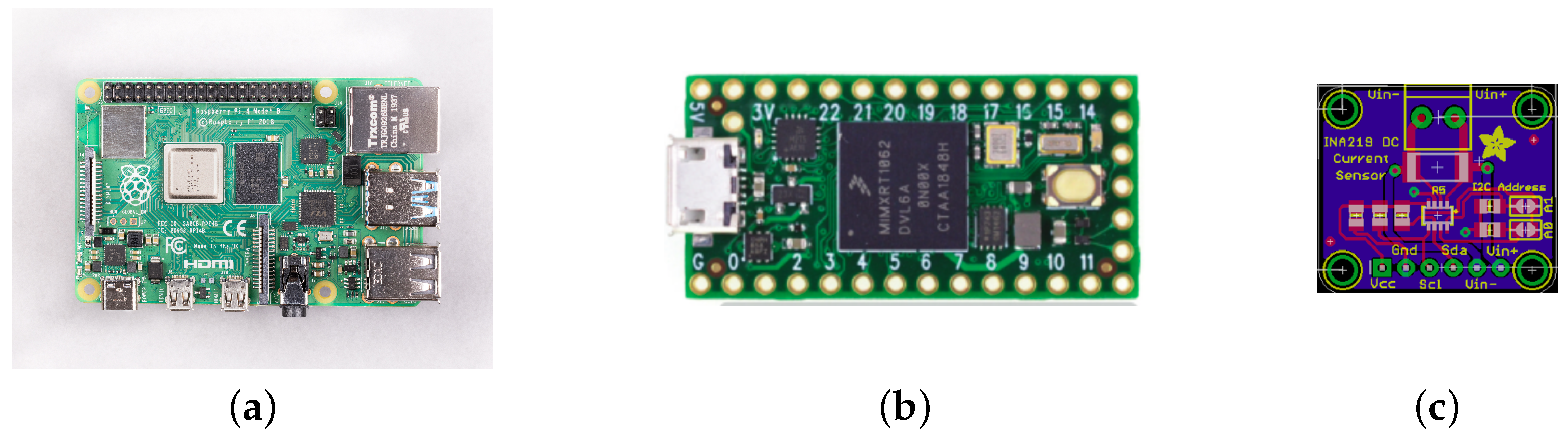
3.1. Device-under-Test and Data Storage Device

Our experimental set-up consists of two Raspberry Pi4 Model B development boards (Raspberry Pi (Trading) Limited, Cambridge, UK) integrated with Broadcom BCM2711, Quad-core Cortex-A72 (ARM v8) 64-bit system-on-chip processors (Broadcom Inc., San Jose, CA, USA) with an internal main reference clock speed of 1.5 GHz. Both Raspberry Pi’s have 32 KB data and 48 KB instruction L1 cache per core, 1 MB L2 cache and 4 GB of LPDDR4-3200 SDRAM. Network connectivity is provided by 2.4 GHz and 5.0 GHz IEEE 802.11ac wireless interfaces, Bluetooth 5.0, 2 USB 3.0 ports and 2 USB 2.0 ports. Each Raspberry Pi provides general-purpose input-output (GPIO) functionality through a 40 pin GPIO header. Each Raspberry Pi is powered over a 5 V DC USB type C connector or 5 V DC GPIO headers. The maximum tolerable current is 3 Amperes [40]. A specification diagram is presented in Figure 1a.

Figure 1. (a) Raspberry Pi4 Model B board peripheral device layout. Detailing position of Broadcom BCM2711 processor, RAM, USB Type-C power supply, and network ports. Source: [41]. (b) Teensy 4.0 microcontroller development board form-factor detailing the positions of the 32 general-purpose input-output (GPIO) pins. Source: [42]. (c) Adafruit INA219 breakout board depicting all pin-out positions. Source: [43].

In addition, operating system loading can be achieved through an embedded Micro-SD card slot. Each Raspberry Pi4 Model B runs the Raspbian Buster Light Debian based distribution of Linux, Kernel version 4.19. The Raspbian Buster Light distribution is a non-windowing version providing only a command-line interface.

3.2. Power, Current, and Voltage Sensing

Power, current, and voltage measurements are achieved by integrating an Adafruit INA219 high side DC sensor breakout board [43] into our tool-chain. The design and specification of the Adafruit INA219 follow that of Texas Instruments’ specification for their INA219 surface-mounted integrated circuit, a small outline integrated circuit (SOIC) form factor [44].

The INA219 contains a precision amplifier that measures the voltage drop across a $0.1\mathsf{\Omega }$ sense resistor, with $1\%$ gain error. The amplifier maximum input difference is $\pm 320$ mV and can measure currents up to $\pm 3.2$ A. Conversions are achieved through an internal 12-bit analog-to-digital converter (ADC), achieving a resolution of $0.8$ mA. A higher resolution can be achieved through the configuration of the internal gain settings, although this reduces the maximum observable current to $\pm 400$ mA, with a resolution of $0.1$ mA [43]. The INA219 is a high side current sensor, requiring that the board be wired with the sense resistor between the load and high voltage and not between the load and the ground.

A pin-out diagram of the breakout board is presented in Figure 1c. The pin-outs being listed from left to right as Vcc, Gnd, Scl, Sda, Vin−, and Vin+; with Vcc and Gnd providing power to the breakout board, Scl and Sda proving $I^{2}C$ clock synchronisation and data transfer; and Vin− and Vin+ allowing the power to the DUT to be routed through the INA219’s sense resistor, remembering to connect Vin− to the high-side of the voltage supply and Vin+ to the high-side of the DUT. A representation of the INA219 block diagram is presented in Figure 1c.

3.3. The Microcontroller

In addition to the two Raspberry Pi4 Model B boards, we integrate into our experimental set-up a Teensy 4.0 microcontroller breakout board (PJRC, Sherwood, OR, USA). The Teensy 4.0 provides dedicated functionality for sampling the current sensor and the transmission of the sampled data to the master Raspberry Pi4 Model B. The Teensy 4.0 microcontroller architecture is built around an ARM Cortex-M7 processor (ARM, Cambridge, UK) with an internal main reference clock speed of 600 MHz. The microcontroller has a 32 KB L1 Data Cache and a 32 KB L1 Instruction Cache, in addition to 1 Mb of RAM and 2 Mb of Flash memory. The board provides access to 32 GPIO pins. The board also has two analog-to-digital converters built on chip. The breakout board also includes real-time clock (RTC) functionality [42]. The Teensy 4.0 form factor is depicted in Figure 1b.

3.4. Experimental Set-Up

To assess the power consumption characteristics associated with the Raspberry Pi load, we must interrupt the direct power supply signal to the load and route the signal through the INA219 current sensor. Powering the Raspberry Pi4 Model B is achieved through a USB Type-C power supply, the official specification defining this supply to be 5 V 3 A. Although the USB Type-C connector’s specification defines many channels, the official Raspberry Pi4 Model B USB Type-C power adapter only contains lines for the high-side 5 V and the low-side ground signal.

These power paths are interrupted (split), and access to their associated signals is achieved using two USB Type-C female breakout boards. Each of the two USB Tyoe-C breakout boards is connected to power through two pin-outs, VBUS and GND, providing 5 V high-side and low-side ground paths, respectively. The USB Type-C pin-out breakout boards also provide pin-outs for all other USB Type-C specification signals, but these are redundant in this set-up. Figure 2 depicts two USB Type-C female breakout boards, showing the power routing configuration.

Figure 2. Integration of two USB Type-C female breakout boards for the interruption of the power supply to the Raspberry Pi4 Model B.

We present the jumper wiring configuration by first detailing the routing of the power signal through the INA219 and to the load, we then detail the integration of the Teensy 4.0 microcontroller to the INA219, and finally0 we detail the procedure for powering the INA219 from the master Raspberry Pi GPIO header pins. Figure 3 provides a detailed breakdown of all jumper wire wirings’ positioning and connection, with each jumper wire numerically labelled for convenience.

Figure 3. The positioning and connection of all jumper wire between master and slave Raspberry Pi4 model Bs and the INA219 current sense amplifier and the Teensy 4.0 microcontroller. [Raspberry Pi4 boards available under a creative commons license: “RaspberryPi 4 Model B.svg” by Jstrom99 CC-BY-SA-4.0].

The power signal routing is achieved by routing the incoming USB Type-C high-side VBUS channel pin-out to the INA219’s Vin+ pin-out, jumper wire ‘1’. Internally, this high-side current is then directed through the INA219’s internal circuitry’s bus lines to the integrated sense resistor and back to the INA219’s Vin- pin-out. The INA219’s Vin- high-side 5 V signal is reconnected to the second USB Type-C high-side VBUS pin-out, jumper wire ‘2’—thus reconnecting/completing the high-side 5 V path. Concerning the low-side ground signal, there is no routing other than to connect both USB Type-C GND pin-outs, jumper ‘3’—thus directly reconnecting/completing the low-side ground path. Finally, due to the technique of high-side sensing of the load, the Raspberry Pi4 needs to be grounded relative to the INA219’s configuration, jumper ‘4’.

Configuring the $I^{2}C$ clock and data lines between the INA219 and the Teensy 4.0 microcontroller involves connecting the INA219 serial clock pin-out (Scl) to the Teensy 4.0 microcontroller’s GPIO pin 19, jumper ‘5’. The INA219 serial data pin-out (Sda) is connected to the Teensy 4.0 microcontroller’s GPIO pin 19, jumper ‘6’. Teensy 4.0 microcontroller power is achieved through USB.

The INA219 high-side current sensor is powered from the master Raspberry Pi. A high-side 5 V signal is routed from the Raspberry Pi’s GPIO header pin ‘2’ to the INA219’s Vcc pin-out, jumper ‘7’. Finally, a low-side ground signal is routed from the Raspberry Pi’s GPIO header pin ‘6’ to the INA219’s Gnd pin-out, jumper ‘8’.

This configuration ensures that all circuitry components are powered from devices isolated from the load of the Raspberry Pi. An image of the actual bench set-up is shown in Figure 4.

Figure 4. Experimental bench set-up, showing two Raspberry Pi model B, INA219 current sensor, and a Teensy 4.0 microcontroller; all wired as described in Experimental Set-up.

3.5. Statistical Analysis

In this section, we list the statistical techniques used regarding the generation of results.

All variables’ distributions were characterised descriptively through time series plots, histograms, box-and-whisker plots, and error bars. Furthermore, each distribution was descriptively summarised using the usual five-point statistics alongside their respective mean, standard deviations, and confidence intervals. Statistical differences in distribution parameters, such as the mean, were assessed using Independent Sample t-tests for testing the differences between two groups. In the cases were distributions violated parametric assumptions, Mann–Whitney tests of the differences in medians was performed. Assessing for differences across more than two groups: an Analysis of Variance was undertaken. Testing for differences between more than two medians, the Kruskal–Wallis tests were were performed. Multiple linear regression models were developed for the regressing of power consumption. The dependent variable being power consumption, and independent variables consisting of CPU core frequency, bare-metal\operating system model category, and the magnitude of power measurements—low, medium, and high.

Regarding assessing the distributional substructure, a parametric statistical change point analysis was undertaken. A comprehensive overview of the underpinnings of the technique can be found in [45]. With that said, we provide a conceptual overview of its application in this research.

In Figure 5a, we present a time series plot of 20,000 power measurements, the horizontal axis indexing those measurements in time, with the vertical axis representing the magnitude of the observations in mW. The figure has been superimposed with three coloured bands (envelopes), coloured yellow, red, and purple. The yellow envelope (low-power) circumscribes a sequence of power measurements associated with power magnitudes less than those circumscribed within the red envelope (mid-power). The purple envelope (high-power) circumscribes measurements that have power magnitudes greater than those in the red envelope and those within the yellow envelope.

Figure 5. Sub-plot (a) defines the concept of a power envelope, plot (b) showing a graphical result of applying a change point analysis.

We were interested in finding the power consumption magnitudes that demarcate each of the power phase envelopes and as such we analysed the sequence of power consumption measurements. The sequence of measurements was first ordered from smallest to largest, the result of which is presented in Figure 5b. The black-lined curve is representing those measurements. The ordering ensured that all low-power envelope observations would precede mid-power envelope observations and that mid-power phase envelope observations would precede those falling within the high-power phase envelope.

The change point analysis consumes observations from left-to-right, adding them to a temporary distribution. That distribution is compared to a distribution that contains all other values (those values all having a greater magnitude than those found within the first distribution). A change point represents a point along the horizontal axis with the property that all values less than the change point is associated with a distribution with a statistically significant different mean and variance compared to the distribution of observations that follow the change point. The analysis is based on Maximum Likelihood estimates of the distributional parameters.

In Figure 5b, the two horizontal red lines run across the measurements that form both distributions. The lower horizontal red-line is running across a sequence of measurements, forming the first distribution. The higher horizontal red-line is running across a sequence of measurements, forming the second distribution. The two vertical double-ended arrow lines running parallel beside the y-axis are superimposed to depict the power consumption magnitudes composing each of the two identified distributions.

All statistical analysis was done using RStudio Version 1.3.1073 [46]. Change point detection was undertaken using the R package “changepoint” [47].

In the next section, we detail the results of this research.

4. Results

This section presents the results from an analysis of a Raspberry Pi4 Model B development board’s baseline idle power consumption characteristics. We consider seven models of baseline idle system state. The first three detail our findings in relation to the capturing of power consumption measurements driving a baseline machine running on bare-metal with no booted operating system. The first two bare-metal cases are associated with the boot cycle failing to find a kernel to load, the power consumption characteristics of these two cases are considered with and without the inclusion of the power overhead associated with the integration of a cooling fan. The third bare-metal case is associated with a full boot cycle, with a minimal kernel boot. The minimal kernel instructs the firmware to activate the data cache, instruction cache, and branch prediction unit. We then present our findings concerning four models of power consumption characteristics for the Raspberry Pi4 Model B, running an out-of-the-box distribution of the Raspbian Linux operating system. Those models considering four different processor core clock frequencies set at 600 MHz, 900 MHz, 1200 MHz, and the default 1500 MHz.

Our findings are presented from two perspectives. The first perspective concentrates on the totality of power consumption measurements associated with each case and identifying overall distribution characteristics. The second focuses on the identification of the composite distributions present within the overall power consumption traces. In particular, we present a detailed overview of our findings associated with a change-point analysis of the overall distribution structure, supporting the identification of composite distribution boundaries within the overall power consumption traces. We present graphical representations of all distributions using time-series plots, distribution histograms, and distribution box-and-whisker plots for both lenses. We then present a numerical summary of all distributions using the typical five-point quartile summary, alongside distribution mean power consumption and their associated standard deviations. We also test for differences in average and median power consumption characteristics grouped by case and clock frequencies. Finally, we present the results of an analysis of the measurements recorded below the INA219 high-side current sense amplifier’s resolution.

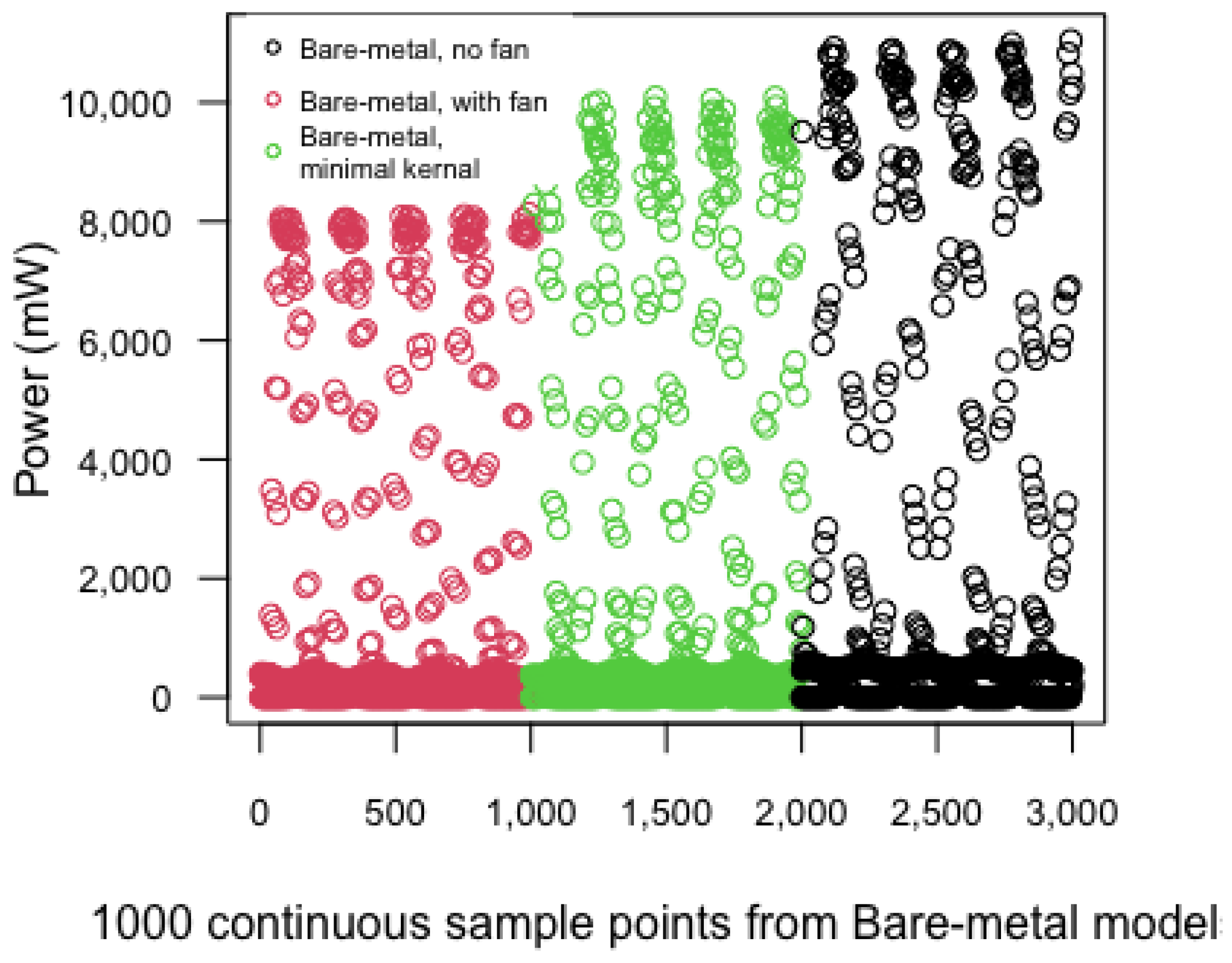
4.1. Bare-Metal Power Distribution Characteristics

In this section, we present our results from the analysis of the power consumption characteristics of a Raspberry Pi4 Model B, powered with no operating system, with and without the overhead associated with a cooling fan.

In Figure 6, we present three panels: (a), (b) and (c), with each composed of three time series scatterplots representing power consumption profiles detailing a sample of 20 K continuous measurements, 2 K of continuous measurements, and a sample of 200 continuous measurements. The vertical axis in all cases representing power in mW. Panel (a) is associated with a Raspberry Pi4B powered on bare-metal with no kernel boot and no cooling fan, with panel (b) representing the characteristics associated with the inclusion of the additional overhead of a cooling fan, and panel (c) representing the power consumption characteristics associated with a Raspberry Pi4B powered on bare-metal with an embedded kernel boot. The embedded kernel provides instruction to the firmware to activate the data cache, instruction cache, and branch prediction unit. Inspection of all three panels highlights the presence of three distinct power consumption phase envelopes.

Figure 6. Time series scatterplots of the power consumption profiles of a Raspberry Pi4 powered on bare-metal. Panel (a) representing the case with no kernel boot excluding a cooling fan, panel (b) the case with no kernel boot with the addition of a cooling fan, and panel (c) representing the case with an embedded kernel boot with the kernel activating the data cache, instruction cache, and branch prediction unit. Each panel presents three granularities of focus, (i) continuous samples 20 K observations, (ii) a continuous sample of 2 K observations, and (iii) a continuous sample of 200 observations.

Inspection of the scatterplots descriptively indicates that the low power consumption phase (dark band of measurements) ranges between 0 W and approximately 1 W, irrespective of the model. The mid-level power consumption phase, showing the largest dispersion, ranges between 1 W and approximately 7 W in the case of no fan. The inclusion of a cooling fan bare-metal case and the bare-metal case with an embedded kernel booted showing similar power consumption ranges between 1 W and 9 W. Considering the high powered phases, maximum power consumption peaks at approximately 8 W in the no fan case, at 10 W when a cooling fan is powered on, and peaks at approximately 11 W for the case when a minimal kernel has booted.

Overall, Figure 7 shows a progressive increase in power measurement ranges moving across the cases from left to the right. These results show the isolation of the distribution of idle power post kernel boot and the increase in power measurement dispersion as the Raspberry Pi4 boot phase successfully loads an appropriate kernel and powers up the data cache, instruction cache, and branch prediction circuitry. Interestingly, although the inclusion of a cooling fan has the effect of increasing the width of the power consumption range relative to the pure bare-metal cases with no kernel boot and no cooling fan, the booting of a successful kernel has a greater effect in increasing the width of the range associated with our measurements.

Figure 7. Time series scatterplots contrasting the different power consumption distribution range across the three bare-metal implementations, providing a side-by-side representation of the dispersion of power measurements with the bare-metal no kernel boot represented in green scatter-dots, the inclusion of a cooling fan case represented by black scatter-dots, and the bare-metal case consisting of an embedded kernel boot presented as red scatter-dots.

Similar distributional ranges are evident across all three cases when focusing on the individual power consumption phase envelopes. No descriptive difference is evident concerning the widths of the low-power phase envelopes, all having a similar dispersion. On the other hand, the mid-power phase envelopes tend to widen as we progress from left to right across the three bare-metal models. A similar trend is present concerning the high-power phase envelope ranges. In summary, the transition through the boot process up to a successful kernel boot affects the magnitude of dispersion present within the composite distributions.

4.1.1. Numerical Descriptive Characteristics of Bare-Metal Power Consumption Distributions

The typical five-point summary of the bare-metal Raspberry Pi4 cases’ power consumption characteristics, alongside the usual mean and standard deviations associated with the power consumption distributions, are presented in Table 1.

Table 1. Descriptive statistics associated with the full sample of power measurements for a bare-metal Raspberry Pi4 powered with and without a cooling fan and a minimal kernel boot. Presenting the minimum power consumption observed (Min), the power measurement associated with the distributions’ first quartile (Q1), median (Md), third quartile (Q3), the largest observed power consumption (Max), alongside the mean (M) and associated standard deviation (SD). All results reported in mW.

Descriptive Point Summary
Cooling Fan	Min	Q1	Md	Q3	Max	M	SD
Bare-metal (no fan)	0.0	26	328	421	8365	1392	2513
Bare-metal (with fan)	0.0	23	386	517	10,398	1697	3033
Bare-metal (with kernel)	0.0	261	491	630	11,026	1886	3259

It is clear on inspection of the five-point numerical summary that lower quartile distribution ranges are similar between both cases in which the boot cycle failed to locate a minimal kernel, differing by at most 3 mW. In contrast, the boot cycle’s completion with a minimal kernel load has had the effect of pushing the first quartile measurement point to a higher power consumption magnitude, specifically; 261 mW. Greater divergence is noted between the power consumption distributions as we progress further through the quartile measures. In particular, the effect from the inclusion of a cooling fan, bare-metal with Fan case, results in an increase in median power consumption to $M_d=386$, an increase of approximately 58 mW in contrast to the median power consumption of the powered Raspberry Pi4 with no fan ($M_d=328$). Considering the bare-metal with Kernel case, median power consumption magnitude also shows an increase above and beyond what was observed relative to the two cases with no successful kernel load. These results allow us to characterise Raspberry Pi4 power consumption associated with the GPU, which predominately is involved in the early stages of the boot cycle, with the effect of adding a minimal kernel that activating cache and branch prediction. At the third quartile measurement level, similar increases in power consumption magnitudes are observed between models. Moving across the three models, we see a similar trend concerning peak power consumption, with consumption magnitudes increasing from approximately 8 W to 10 W and 10 W to 11 W.

Although the aforementioned five-point summary of the power distributions would offer a fairer understanding of distributional characteristics due to their extreme positive skew, as presented in Figure 8, average power consumption is predominately conveyed within the literature. As such, we also present our findings in that regard. Inspection of average power consumption magnitudes similarly suggests an increase in distributional point-estimates as we progress through the boot cycle. The inclusion of a cooling fan or the boot cycle’s completion has the effect of shifting the mean power distributions to higher magnitudes. The average power consumption without a cooling fan is approximately $1.39$ W in contrast to the $1.70$ W associated with the inclusion of a cooling fan, the full boot cycle completion resulting in an average power consumption magnitude of approximately $1.9$ W.

Figure 8. Histograms depicting the power consumption distributions associated with a bare-metal Raspberry Pi4 powered (a) without kernel boot and no cooling fan; (b) without kernel boot and an included cooling fan; and (c) with an embedded kernel boot.

Inspection of histogram representations of the bare-metal power consumption distributional characteristics, presented in Figure 8, show similar trends across all bare-metal cases. Specifically, all cases exhibit excessive positive skewness in their distributions. Considering the low magnitude observations less than 1000 mW, the two cases associated with no kernel boot, plots (a) and (b), show that approximately $75\%$ of their measurements are below 500 mW. In contrast, the minimal kernel boot case, plot (c), shows a redistribution of approximately $15\%$ of measurements into the range between 500 mW and 1000 mW.

An alternative representation of the power consumption distributions for each of the three bare-metal cases showing the extreme positive skewness and the predominance of power consumption magnitudes falling below 1000 mW, as depicted within Figure 9a.

Figure 9. (a) Box-and-whisker plots depicting the power consumption distributions for each of the three bare-metal cases. (b) Confidence intervals of $95\%$ for the population means for each of the three bare-metal cases.

4.1.2. Differences between Bare-Metal Power Consumption Distributions

This section presents our findings from analysing the statistical differences in the power consumption distributions between the three bare-metal cases.

Due to the presence of extreme positive skewness within all three distributions, the non-parametric Kruskal–Wallis H test was undertaken to assess if there was a statistically significant difference in median power consumption magnitudes between all bare-metal cases. The results of the Kruskal–Wallis H test indicate differences in median power magnitudes between the three bare-metal model, ${\chi }^2=3142.8$, $df=2$, $p<0.001$. Post-hoc Mann–Whitney tests indicate statistically significant differences in pairwise medians across all groupings, all p’s $<0.001$.

An analysis of the $95\%$ confidence intervals for the respective bare-metal case population means, as presented in Figure 9 would indicate that average power consumption between cases is statistically significantly different, at the $5\%$ level of significance, a characteristic inferred from the non-overlap in relative confidence intervals.

4.2. Distribution Characteristics Associated with a Booted Operating and Varying Underclocking Frequencies

In Figure 10, we present three different granularities of observation within each panel, from left to the right representing the full 20 K trace of power consumption measurements, with each panel’s centre scatterplot representing a continuous 2 K sample of measurements. Finally, the far-right scatterplot in each panel represents 200 continuous samples of measurements. In all cases, the horizontal axis represents time and, in particular, continuous sample points. The vertical axis represents power as measured in milli-watts (mW).

Figure 10. Time series scatterplots depicting power consumption of a Raspberry Pi4 with a fully booted operating system, running at clock frequencies of 1500 MHz (panel a), 1200 MHz (panel b), 900 MHz (panel c), and at 600 MHz (panel d).

Similar to the characteristics associated with power consumption at baseline with no operating system, running with or without a cooling fan (Figure 6); irrespective of clock frequency, each distribution of power consumption measurements are distributed within three phase bands. These three bands are more evident when each panel’s centre plot, labelled (ii), is inspected.

Irrespective of clock frequency, the lower power consumption envelope in all cases is within a range of between 0 W and 1 W. Similarly, in all cases, irrespective of clock frequency, the mid-power consumption envelope measurements range between 1 W and 10 W. Finally, all high-power consumption envelopes have a similar range of measurements, falling within a range of between 10 W and 12 W.

4.2.1. Numerical Distribution Characteristics Associated with a Booted Operating and Varying Underclocking Frequencies

The results from a descriptive numerical analysis of the power consumption characteristics associated with the Raspberry Pi4, powered with a booted Operating System, with the processor running at 600 MHz, 900 MHz, 1200 MHz, and 1500 MHz clock frequencies are presented within Table 2. No observable trend is present with respect to comparisons across clocking frequency first quartile measurements. In contrast, median power consumption magnitudes increase as we progress across clocking frequencies, although the range of increase is small, representing 31 mW between the 600 MHz case and the 1500 MHz case. Similar increases in power consumption measurements are associated with third quartile values, with them spanning a range of approximately 41 mW from the 600 MHz to 1500 MHz clock frequencies.

Table 2. Descriptive statistics associated with the full sample of power measurements for a Raspberry Pi4 with a booted Operating System, associated with each of the four clock frequencies 600 MHz, 900 MHz, 1200 MHz, and 1500 MHz. Presenting the minimum power consumption observed (Min), the power measurement associated with the distribution’s first quartile (Q1), median (Md), third quartile (Q3), the largest observed power consumption (Max), alongside the mean (M) and associated standard deviation (SD). All results reported in mW.

Descriptive Point Summary
Clock (MHz)	Min	Q1	Md	Q3	Max	M	SD
600 MHz	0.0	178	446	553	12,304	1967	3523
900 MHz	0.0	261	462	582	13,758	2087	3694
1200 MHz	0.0	183	468	585	13,016	2064	3700
1500 MHz	0.0	122	477	596	12,958	2073	3720

An analysis of the mean power consumption magnitudes having a dispersion within a range of 120 mW across clock frequencies. On average, mean power consumption magnitudes are approximately 5 times larger than median summaries. Interestingly, standard deviations are approximately 10 times larger than the interquartile summaries.

4.2.2. Difference Effects Due to Booted Operating System at Varying Clock Frequencies

An analysis of the differences in mean total power consumption are presented through plots of test case $95\%$ confidence intervals for population means in Figure 11a. It is evident from the plot that there is non-overlap between the $95\%$ confidence intervals associated with the power consumption observations for the 600 MHz, and 900 MHz cases, indicating statistically significant differences in their respective population means. The cases 900 MHz, 1200 MHz, 1500 MHz show no differences in population mean power consumption magnitudes.

Figure 11. Error bar plots depicting $95\%$ confidence intervals associated with population means for each model, plot (a); and Box-and-whisker plots depicting distribution medians and associated quartiles, plot (b).

A Kruskal–Wallis rank-sum test was conducted to assess if there were statistically significant differences in median power consumption measurements between each of the four clock frequency cases. The results of the Kruskal–Wallis H test indicate that there is a statistically significant difference in median power measurements between clock frequencies, (${\chi }^2=227.75$, $df=3$, $p<0.001$). Box-and-whisker plots of each distribution are shown in Figure 11b. It is evident from each box-and-whisker plots that power consumption magnitudes are predominately less than approximately 1000 mW. In addition, the excessive positive skewness, signified by the long vertical black sequence of observations, would indicate that any over-reliance on the mean for point-estimates of power consumption would introduce a large degree of uncertainty into relative power consumption models.

4.3. Power Phase Envelope Bounds Detection

In order to determine the boundary values associated with each of the three identified power phase envelopes, a change-point analysis was undertaken on each trace of power consumption observations. All results are presented in Figure 12 panels (a) through to (g).

Figure 12. Scatterplots depicting ordered power consumption magnitudes and the identification of distribution turning-points. Superimposed over each plot are two horizontal red lines—the lower red line running over the sequence of observations that compose the first distribution. The higher red horizontal line runs across the sequence of observations with distributional characteristics statistically significantly different from those associated with the lower red line. Sub-panel plot (i), in all cases, depicting the sequence of power consumption observations recorded with a magnitude of 0 mW. This sequence is representing measurements below the resolution of the INA219. Sub-panel plot (ii), in all cases, identifies the turning point associated with the low-power phase envelope upper bounds. Each sub-plot (iii) represents the turning point associated with the mid-power phase envelope upper bounds and represents the lower bound limit associated with the high-power phase envelopes.

A detailed overview of the boundaries associated with the three power phase envelopes identified through the change-point analysis is presented for each model in Table 3. For example, in the 600 MHz case, the low phase power envelope had a range between 0 mW and 782 mW, with a mid-power phase envelope ranging between 782 mW and 10,558 mW, the upper-power phase envelope ranging between 10,588 mW and 12,304 mW.

Table 3. Power consumption phase envelope boundaries, with 1st $CP$ representing the first identified change-point, and 2nd $CP$ representing the second identified change-point. Sub-distributions coincide as: low phase envelope—[Min, 1st $CP$), mid phase envelope—[1st $CP$, 2nd $CP$), and the third phase envelope consists of power consumption magnitudes within the interval [2nd $CP$, Max].

Model	Min	1st $\mathit{C}\mathit{P}$	2nd $\mathit{C}\mathit{P}$	Max
Bare-metal (no fan)	0	594	7627	8365
Bare-metal (with fan)	0	673	9039	10,398
Bare-metal (with kernel)	0	839	8090	11,040
600 MHz	0	782	10,558	12,304
900 MHz	0	801	11,382	13,758
1200 MHz	0	832	11,241	13,016
1500 MHz	0	862	11,162	12,958

An inspection of the low-power phase envelopes, demarcated by the min and 1st $CP$ values, indicate a progressive widening of the power consumption ranges stepping through the models associated with the bare-metal cases. A similar trend is present across the 600 MHz to 1500 MHz operating system cases. With that said, peak power associated with the bare-metal case running a minimal kernel has a magnitude greater than the 1200 MHz operating system case but below the peak power associated with the 1500 MHz operating system case. An alternative representation of these trends being presented through bar charts in Figure 13a.

Figure 13. Bar charts depicting phase envelope ranges for the low-power phase envelope (a), the mid-power phase envelope (b), and the high-power phase envelope (c).

Focusing on mid-power phase envelope characteristics: their lower bounds are presented in the column labelled 1st $CP$, and their associated upper bounds are presented in the column labelled 2nd $CP$ of Table 3. Our results show that peak mid-power phase envelope magnitudes exhibit an umbrella effect for both the bare-metal and the booted operating system cases. Contrasting the bare-metal cases with the operating system cases: our results show that mid-power phase envelope ranges are narrower for the bare-metal cases. Furthermore, our results show that the mid-power phase envelopes are, on average, 12 times wider than their associated low-power phase envelope widths. On average, the mid-power phase envelopes have a range of approximately 9000 mW. These trends can also be examined within the bar chart presented in Figure 13b.

The increasing effect and the umbrella effect identified within the low-power and mid-power phase envelopes can also be found within the high-power phase envelope results. Bare-metal cases showing widening of high-power phase envelope ranges, whereas the operating system cases show an umbrella effect. Figure 13c depicting both effects.

4.3.1. Power Consumption Proportions between and within Each Power Phase Envelope

An analysis of the proportion of observations falling within each of the three power phase envelopes was undertaken for all models, the results of which are presented in Table 4.

Table 4. The proportion of power phase envelope observations falling within the low-power phase envelope ($P_{low}$), the mid-power phase envelope ($P_{mid}$), and the high-power phase envelope ($P_{high}$).

Model	${\mathit{P}}_{\mathit{l}\mathit{o}\mathit{w}}$	${\mathit{P}}_{\mathit{m}\mathit{i}\mathit{d}}$	${\mathit{P}}_{\mathit{h}\mathit{i}\mathit{g}\mathit{h}}$
Bare-metal (no fan)	78	15	8
Bare-metal (with fan)	76	16	8
Bare-metal (with kernel)	77	11	12
600 MHz	78	16	7
900 MHz	77	17	5
1200 MHz	78	17	6
1500 MHz	78	15	7

Regarding the low-power phase envelopes, on average, approximately $77.3\%$ of power measurements fall within each model’s low-power phase envelope. The results of a 7-sample test for equality of proportions indicating that there was a statistically significant difference between the proportions observed, ${\chi }^2=19.234$, $df=6$, $p<0.005$. With that said, the proportions differed by no more than $2\%$.

Considering mid-power phase envelope proportions, these ranged between approximately $11\%$ and $17\%$ of power consumption observations. The results of a 7-sample test for equality of proportions indicate that there was a statistically significant difference between the proportions observed, ${\chi }^2=896.46$, $df=6$, $p<0.001$. The proportions differ by no more than approximately $2\%$.

Concerning high-power phase envelopes, approximately $6.7$ of power consumption measurements lie within their respective high-power phase envelopes. The results of a 7-sample test for equality of proportions indicated that there was a statistically significant difference between the proportions observed, $ch{i}^2=1530.9$, $df=6$, $p<0.001$. Similar with the low power phase envelope, the proportions differed by no more than $3\%$.

4.3.2. Descriptive Characteristics of Power Phase Envelopes

An analysis of the numerical descriptive characteristics for each model was undertaken with a specific focus within each of the three power phase envelopes, the results of which are presented in Table 5. For example, the 900 MHz mid-power envelope is associated with a minimum power consumption of 802 mW, with $25\%$ of observations within that envelope being less than 4105 mW, the median power consumption is 6838 mW, $75\%$ of the band’s observations being less than 10,334 mW, the 990 MHz envelope recording a peak power consumption value of 11,380 mW, on average power consumption within the envelope being 6830 mW with an associated standard deviation of 3378 mW. The $95\%$ confidence interval for the population mean having a lower bound of 6712 mW and an upper bound of 6948 mW.

Table 5. The power phase envelope descriptive statistics associated with low, mid, and high power phase envelope cases. The first column, labelled Phase, lists the three power phase envelopes; the second column, labelled Model, lists the six system cases; the following five columns list the usual quartile descriptives; the final three columns list distribution mean, standard deviation, and respective model $95\%$ confidence intervals for the population mean power consumption. All results reported in mW.

Phase	Model	Min	Q1	Md	Q3	Max	M	SD	CI(95)
Low	Bare-metal (no fan)	0	0	294	351	594	218	163	(216, 221)
	Bare-metal (with fan)	0	0	341	411	673	254	191	(251, 257)
	Bare-metal (with kernel)	0	0	460	499	836	340	227	(336, 343)
	600 MHz	0	0	394	478	778	304	215	(301, 308)
	900 MHz	0	0	413	499	801	322	221	(318, 325)
	1200 MHz	0	0	414	505	828	321	226	(318, 325)
	1500 MHz	0	0	417	510	861	323	233	(319, 327)
Mid	Bare-metal (no fan)	595	1843	4363	6554	7621	4197	2369	(4113, 4281)
	Bare-metal (with fan)	675	1897	5040	7664	9038	4874	2858	(4779, 4970)
	Bare-metal (with kernel)	839	1710	3845	6058	8075	3998	2317	(3901, 4096)
	600 MHz	782	3051	6893	9566	10,554	6294	3340	(6171, 6417)
	900 MHz	802	4105	6838	10,334	11,380	6830	3378	(6712, 6948)
	1200 MHz	832	3527	7528	10,498	11,241	6917	3582	(6790, 7045)
	1500 MHz	862	3370	7019	10,039	11,158	6605	3455	(6475, 6736)
High	Bare-metal (no fan)	7627	7795	7894	8019	8365	7913	153	(7906, 7921)
	Bare-metal (with fan)	9039	9284	9508	9721	10,398	9523	283	(9509, 9537)
	Bare-metal (with kernel)	8090	9038	10,101	10,370	11,026	9791	756	(9761, 9821)
	600 MHz	10,558	10,777	10,988	11,224	12,304	11,015	296	(10,999, 11,032)
	900 MHz	11,382	11,647	11,906	12,186	13,758	11,951	375	(11,928, 11,974)
	1200 MHz	11,242	11,433	11,618	11,838	13,016	11666	301	(11,647, 11,684)
	1500 MHz	11,162	11,377	11,559	11,777	12,958	11,592	278	(11,577, 11,607)

Focusing on low-power phase envelope mean and median power consumption magnitudes, similar trends are evident within the bare-metal cases and within the cases that included an operating system boot. Specifically: both sets of cases showing increasing mean and median power consumption magnitudes progressing through their associated configurations. The increase is more pronounced, transitioning from the bare-metal case with no cooling fan to the bare-metal case running with a minimal kernel, representing a change of 166 mW in median magnitudes and 122 mW mean magnitudes. In contrast, a change of approximately 20 mW was observed relative to the cases that included an operating system boot. With that said, the bare-metal case running a minimal kernel showed the greatest mean and median power consumption at the low-power phase level compared to all other cases. We should also highlight that the low-power phase envelopes are associated with approximately $78\%$ of all observations, as noted in Table 4.

Analysing the results associated with mid-power phase envelopes, which on average represent approximately $15\%$ of observations, umbrella effects are present across mean and median power consumption magnitudes within the bare-metal cases and within the cases that included an operating system boot. With that said, mid-power phase mean and median magnitudes for the cases that included an operating system boot are, on average, approximately 1500 mW larger than the average mid-power phase magnitudes associated with the bare metal cases.

A similar trend is evident to that found for mid-power phase mean, and median magnitudes compared to high-power phase mean and median magnitudes. Albeit, high-power phase mean and median magnitudes for the cases that included an operating system boot are, on average, approximately 2400 mW larger than the average mid-power phase magnitudes associated with the bare metal cases.

A box-and-whisker plot representation of all three power phase envelope cases is presented in Figure 14.

Figure 14. Box-and-whisker plots depicting power consumption phase envelope distributions associated with low, mid, and high-power phase envelope cases. Low-power phase envelope (a), mid-power phase envelope (b), and high-power phase envelope (c).

4.3.3. Differences in Mean and Median Power Phase Envelope Magnitudes

An analysis of the differences in mean power phase envelope magnitudes was undertaken by assessing case phase level $95\%$ confidence intervals for their associated population means. The results are presented in Figure 15.

Figure 15. Error bar plots depicting $95\%$ confidence interval for population means for each model. Low power phase envelope (a), mid power phase envelope (b), and high power phase envelope (c).

Focusing on the characteristics of mean low-power phase envelope magnitudes: it is evident from the non-overlap across all three bare-metal cases’ $95\%$ confidence intervals that statistically significant differences in mean power consumption exist. Considering the no operating system boot cases: only the 600 MHz case shows statistically significant differences in mean power consumption magnitudes compared to the 900 MHz, 1200 MHz, and 1500 MHz cases. As identified in the previous descriptive analysis, the bare-metal case with a minimal kernel boot shows statistically significant differences in mean power consumption compared to all other cases.

Assessing these differences non-parametrically: a Kruskal–Wallis H test was undertaken to assess if there was evidence to suggest that median low-power phases are different between cases. The results indicate statistically significant differences in median low-power phase envelope magnitudes between each of the six models, ${\chi }^2$ = 11,559, $df=6$, $p<0.001$. Post-hoc independent samples Mann–Whitney tests for the difference in medians, indicating that all pairwise comparisons in median low-power phase magnitudes were statistically significantly different (all p’s $<0.05$).

Considering mid-power phase envelope magnitudes, Figure 15b: considering the three bare-metal cases, the previously identified umbrella effect is evident; with that said, no overlap is present across any of the three $95\%$ confidence intervals indicating statistically significant differences in mean low-power phase consumption magnitudes between those cases. A similar trend to that observed for the low-power phase, no operating system cases are evident. Only the 600 MHz case indicating a statistically significant difference in mean power consumption magnitude compared to the other no operating system cases.

A non-parametric Kruskal–Wallis assessment of median mid-power level magnitudes indicates the presence of statistically significant differences between median values, ${\chi }^2=3189.9$, $df=3$, $p<0.001$. A post hoc Mann–Whitney analysis was undertaken to identify all pairwise differences in median power consumption magnitudes across test cases. Except for the pairwise analysis between the 900 MHz and 1200 MHz cases, all showed statistically significant differences between their median power consumption magnitudes (all p’s $<0.001$).

Finally, similar to the low and mid-power phase envelopes, high-power phase envelopes median magnitudes are statistically significantly different between cases, ${\chi }^2=8357.2$, $df=3$, $p<0.001$. Follow up post hoc Mann–Whitney independent sample tests identified all pairwise comparisons to be statistically significantly different (all p’s $<0.001$).

4.3.4. Power Phase Envelope Transitions

An analysis of the degree to which power consumption magnitudes reside within their phase envelopes or transition between respective power phase envelopes was undertaken. The results of which are presented in Table 6.

Table 6. Phase level transitions between low, mid, and high-power phase envelope boundaries. Detailing the proportion of transitions for the three bare-metal models, two of which had no kernel boot—no cooling fan (BM-NF) and addition of a cooling fan (BM-WF); the third including the boot of a minimal kernel powering cache an branch prediction units (BM-MK). Furthermore, the proportion of transitions associated with the four frequency scaling models associated with a full operating system boot.

	Bare Metal (%)			Booted Operating System (%)
Transition	BM-NF	BM-WF	BM-MK	600 MHz	900 MHz	1200 MHz	1500 MHz
(low, low)	55.2	52.8	54.1	55.2	54.3	55.3	55.8
(low, mid)	14.8	16.0	10.7	15.6	17.4	16.7	14.8
(mid, low)	14.8	16.0	10.7	15.6	17.4	16.7	14.8
(low, high)	7.6	7.8	12.2	6.8	5.4	5.7	7.3
(high, low)	7.6	7.8	12.2	6.8	5.4	5.7	7.3

The results indicate that approximately between $53\%$ and $56\%$ of transitions stay within their associated low-power phase envelope, irrespective of the model. Interestingly, transitions to higher power consumption phases all originate from the low-power phase regions. There were no transitions observed from mid-power phase regions to high-power phase regions and none from the high-power phase regions to the low-power phase regions.

4.4. Power Consumption Models

A multiple linear regression was undertaken to predict average power consumption, regressing power consumption measurements on CPU core frequency, bare-metal\operating system cases, and power phase envelope level. The results indicated that variation in CPU core frequency, bare-metal\operating system case, and power phase envelope levels account for $97.6\%$ of the average power consumption variation ($R^2=0.976$). The overall model was statistically significant, $F(4,16)=161.997$, $p<0.001$. The predictor “model,” representing the bare-metal or booted operating system cases, was identified as a statistically significant predictor of average power consumption, $t=4.000$, $p<0.05$. The dummy variable, “low-phase,” coding the low-power phase observations, was also identified as a statistically significant predictor of average power consumption, $t=-24.982$, $p<0.001$. Similarly, the dummy variable, “mid-phase,” coding the mid-power phase observations, was identified to be a statistically significant predictor of average power consumption, $t=-11.81$, $p<0.001$. CPU core frequency was not found to be a statistically significant predictor.

In contrast to the above model, we regressed the overall average power consumption measurements on CPU core frequency and bare-metal\operating system cases. Although the model accounted for $67.2\%$ of the variation in power consumption measurements, the results failed to reach statistical significance, $F(2,4)=4.102$, $p=0.107$.

4.5. Power Consumption Measurements Outside the Resolution Envelope of the INA219

The distribution of power consumption measurements captured from the INA219 current sensor is reported at a minimum resolution of $0.2$ mW, with real measurements less than $0.2$ mW of power being recorded by the INA219 breakout board as 0 mW.

An analysis of the proportion of such measurements indicates that approximately $24.2\%$ of power measurements for the bare-metal no cooling fan model were recorded as 0 mW. Concerning the bare-metal with a cooling fan model, $24.6\%$ of power measurements were recorded as 0 mW. In the bare-metal case with minimal kernel boot, $20.3\%$ of measurements were recorded as 0 mW. Considering the models with an operating system boot, $22.6\%$, $21.8\%$, $22.2\%$, and $23.0\%$ 0 mW measurements were recorded for clocking frequencies of 600 MHz, 900 MHz, 1200 MHz, and 1500 MHz, respectively.

5. Discussion

The literature concerning the dissemination of power consumption profiles associated with the Raspberry Pi family of development boards is relatively sparse. However, the work of Kaup et al. in [4], Astudillo-Salinas et al. in [3], Bekaroo et al. in [27], Cloutier et al. in [11], and Ardito et al. in [6] do provide a relative baseline from which our results can be benchmarked. All these publications predate the release of the Raspberry Pi4 Model B generation of single-board computer. In this regard, we believe that the present work provides the first detailed distributional assessment of power consumption characteristics of the Raspberry Pi4 model B.

Considering the work of Kaup et al., which focused on analysing a first-generation Raspberry Pi model, their results are interesting compared to those presented within this paper. Their assessment only being comparable relative to our booted operating system cases. Their results report on the relationship between power consumption and CPU utilisation and indicate that at the low levels of CPU utilisation, less than $10\%$, the legacy first-generation Raspberry Pi consumes power within an approximate range of between $1.55$ W and $1.6$ W. Furthermore, at the higher CPU utilisation levels, power consumption peaks approximately in the range between $1.7$ W and $1.75$ W. In contrast, and noting that our results reflect a minimum operating system workload, and thus more comparable with the low CPU utilisation results reported by Kaup et al., the Raspberry Pi4 with its significantly enhanced specification showed an average low CPU utilisation power range of between $1.9$ W and $2.1$ W. Interestingly, our results have shown that when distributional characteristics are considered, and a focus is placed on the low-power phase characteristics, the Raspberry Pi4 predominately consumes power within a power envelope of no more than $0.328$ W at a clocking frequency of 1500 MHz, and averages $0.318$ W. This upper threshold reflects the low-power phase envelope, where the greatest proportion of observations are recorded, representing approximately $78\%$ of measurements.

Focusing specifically on literature that reports on idle power consumption characteristics, detailed distributional characteristics associated with idle power are relatively lacking. Cloutier et al. in [11] do present single point estimates for idle power consumption for several Raspberry Pi generations, in particular, the Raspberry Pi model B, the Raspberry Pi model B${}^{+}$, Raspberry Pi model A${}^{+}$, the Raspberry Pi model 2B, the Raspberry Pi model 3B, and the Raspberry Pi Compute Module. Their results report idle power magnitudes of $2.7$ W, $1.6$ W, $0.8$ W, $1.8$ W, $1.8$ W, and $1.9$ W, respectively, across the aforementioned Raspberry Pi generations. Although the results of Cloutier et al. do not include the Raspberry Pi4 model B, as their analysis is before the release of the Pi4, it is interesting to note that our findings show that the latest Raspberry Pi4 model B, with its enhanced specification, does not surpass the upper magnitudes reported by Cloutier. Our results indicate that the average Raspberry Pi4 Model B power consumption is approximately 2 W, associated with the cases that included a booted operating system.

Similarly, Mao in [13] presents an overview of power consumption characteristics associated with the Raspberry Pi2 generation of board. Their idle power measurements are reported within a range of 1 W and $1.05$ W, derived from an inspection of their time series plot (Mao, Figure 4.2), with average power consumption, reported at $1.048$ W, $50\%$ greater than the results presented within this paper for low-power phase observations for a Raspberry Pi4. Concerning the first generation Raspberry Pi, Mao has reported power consumption magnitudes in the range of between $1.65$ W and $1.75$ W, averaging at $1.70$ W, in contrast to the $2.7$ W reported by Cloutier et al. Putting aside our analysis of average power consumption within each of the three power phase envelopes and erring on the side of caution due to extreme positive skew within our overall distributions, our results show that the Raspberry Pi4 Model B has an idle power magnitude of approximately $1.9$ W. A result between that of Mao and Cloutier et al.

Accurate tests of directional difference between the results in this paper and those reported within the literature would require full reporting of their distributional characteristics. Bekaroo et al. in [27] report on idle power consumption associated with a Raspberry Pi2 model B, among other results. Like those reported by Cloutier et al., their power consumption characteristics are single-point estimates, although their focus was not necessarily on idle power modelling. Their specific results report Raspberry Pi2 Model B idle power at $2.2$ W, a magnitude that would indicate that the result recorded within this paper for the Raspberry Pi4 Model B provides evidence of comparable performance at idle power if not better for the Pi4.

More relevant to the work reported within this paper is communicated by Astudillo-Salinas et al. in [3], in which they report on idle power consumption and, also, the effect of underclocking a Raspberry Pi model B${}^{+}$ on power consumption magnitudes. Similar to the previous studies, no results concerning distributional shape and dispersion are reported. Nevertheless, they report point-estimates for average idle power consumption for the Raspberry Pi model B${}^{+}$ of $1.2$ W. This result is approximately $0.4$ W lower than that reported by Clouiter et al. for the same generation of Raspberry Pi. In respect to underclocking of CPU frequency, their results suggest a reduction in power consumption at lower CPU clock frequencies. More directly comparable to the results within this paper are specifically those of Astudillo-Salinas focusing on the Raspbian Lite operating system. Their results show the greatest power consumption reduction gains for underclocked frequencies, these results showing similar trends to those found in this study. The trend found in this paper regarding the plateauing of power consumption upper bounds is similarly present with respect to the results associated with the Raspberry Pi model B${}^{+}$ booted with the Raspbian lite operating system as communicated by Astudillo-Salina.

Concerning power consumption competition between boards used for embedded applications, and as cited by Alves Filho et al. in [9], the Raspberry Pi has been recognised as “the best option to build a power-aware low cost embedded cluster”. Our results show that of all the cases considered, those assessed with the bare-metal cases showed the most significant reduction in overall power consumption and suggest that, for systems that have a small number of tasks to service, that an actual embedded environment would offer more outstanding power consumption performance.

Our findings show similar power consumption transition behaviour from lower power states to higher power states across all cases regarding all measurements. It should be noted that this behaviour was also observed within the no operating system cases and thus we do not attribute the transitioning behaviour to operating system interrupt routines that need to be serviced. The work of Shizukuishi et al. in [7] would seem to support this proposition. Their findings suggest that Linux build configuration options’ deactivation had no significant impact on power consumption characteristics. A possible alternative explanation that we offer for the transitioning effect would be from the impact of processor package-level and core-level power state transitions.

Finally, the reported results on power consumption associated with Raspberry Pi generation boards are relatively sparse within the literature, differences can be observed between reported magnitudes across similar devices and system setup. We believe that this would support the argument that more detailed distributional analysis is required when analysing power consumption traces, and focus should be directed and given to the effect of distributional shape on the typical statistical point estimates. Our results indicate that, due to the effects of distributional shape on the typical measures of centre and dispersion, a deeper fine-grained analysis of power consumption distributional structure should be undertaken when reporting power consumption results. In that regard, our findings have shown that power consumption traces are a superposition of finer distributions with more conformal characteristics.

More importantly, our results have shown that prediction accuracy concerning power consumption modelling can be significantly increased through the decomposition of overall distributional characteristics into their sub-distributional components. In particular, our findings have shown that the proportion of unaccounted variance associated with failing to consider sub-distributional properties can be increased by 30%, from 67% to 97%.

6. Conclusions

This paper has presented a detailed systematic methodology for sensing and capturing power consumption measurements associated with the latest generation of Raspberry Pi single-board computer, particularly the Raspberry Pi4 model B. This paper presents an in-depth analysis of power consumption distribution characteristics associated with the Raspberry Pi4 Model B powered in a bare-metal configuration, as would be the case for embedded system application development. Alongside this case, the power consumption characteristics associated with the Raspberry Pi4 Model B powered with a booted operating system running across four processor clocking frequencies. In this paper, we have presented a novel approach to the assessment and identification of power consumption distribution boundaries through a distribution change-point analysis from a distributional analysis perspective.

Our results, in general, suggest that the modelling of power consumption characteristics and their inclusion within system power models should consider and include sub-distributional power consumption features. In support of this proposition, our findings identify, irrespective of case, three broad power consumption envelopes associated with idle power consumption. Of these three power phase envelopes, power consumption magnitudes predominately fall within a single low-power phase envelope, and on average, represent approximately $78\%$ of idle power consumption measurements. Our results also highlight significant differences between the power consumption profiles, between cases, depending on whether an operating system boot phase had occurred. In this regard, our results suggest that using a Raspberry Pi4 Model B as an embedded device would result in significantly lower power consumption distributions in contrast to having a booted operating system.

The effect of processor clocking frequencies on Raspberry Pi4 Model B power consumption characteristics suggest that underclocking the device to its lowest possible clocking frequency of 600 MHz, from its default out-of-box clocking frequency of 1500 MHz, affects shifting the power consumption distribution to significantly lower magnitudes. This effect is more dramatic, when the focus is placed on specific power phase envelopes above and beyond the whole distributional characteristics. In particular, from lower-clocking frequencies to higher, power consumption increases dramatically between the lower frequencies, with the effect plateauing across the higher clocking frequencies.

Our findings would place a weight on the importance of assessing full distributional characteristics and err on the side of caution in using the typical mean point-estimates as distributional centre measures, especially without the reporting of associated standard deviations, skewness, and kurtosis estimates.

We would suggest that this work is the first to consider and document the power consumption distributional characteristics associated with a bare-metal Raspberry Pi4 Model B development board. Our results clearly show that bare-metal execution is significantly associated with lower power consumption profiles. Furthermore, we would suggest that this work is the first to consider and document sub-distributional characteristics of power consumption traces through the application of distributional change-point analysis. Our results from this analysis indicate that focusing on overall distributional statistics fails to identify important substructure within power consumption traces.

References

1. Rotem, E.; Naveh, A.; Ananthakrishnan, A.; Weissmann, E.; Rajwan, D. Power-Management Architecture of the Intel Microarchitecture Code-Named Sandy Bridge. IEEE Micro 2012, 32, 20–27. [Google Scholar] [CrossRef]
2. Behr Technologies Inc. BehrTech Blog: Top 10 IoT Sensor Types; Behr Technologies Inc.: Concord, ON, Canada, 2021. [Google Scholar]
3. Astudillo-Salinas, F.; Barrera-Salamea, D.; Vázquez-Rodas, A.; Solano-Quinde, L. Minimizing the power consumption in Raspberry Pi to use as a remote WSN gateway. In Proceedings of the 2016 8th IEEE Latin-American Conference on Communications (LATINCOM), Medellin, Colombia, 16–18 November 2016; pp. 1–5. [Google Scholar]
4. Kaup, F.; Gottschling, P.; Hausheer, D. PowerPi: Measuring and modeling the power consumption of the Raspberry Pi. In Proceedings of the 39th Annual IEEE Conference on Local Computer Networks, Edmonton, AB, Canada, 8–11 September 2014; pp. 236–243. [Google Scholar]
5. Somarribas, J.; Meneses, E.; Olivas, K. Predictive Power Consumption Model for Compute Intensive Applications in Clustered ARM A53 Embedded Systems. In Proceedings of the 2020 IEEE 11th Latin American Symposium on Circuits Systems (LASCAS), San José, Costa Rica, 25–28 February 2020; pp. 1–4. [Google Scholar]
6. Ardito, L.; Torchiano, M. Creating and Evaluating a Software Power Model for Linux Single Board Computers. In Proceedings of the 2018 IEEE/ACM 6th International Workshop on Green Furthermore, Sustainable Software (GREENS), Gothenburg, Sweden, 27 May 2018; pp. 1–8. [Google Scholar]
7. Shizukuishi, T.; Matsubara, K. An Efficient Tinification of the Linux Kernel for Minimizing Resource Consumption. In Proceedings of the 35th Annual ACM Symposium on Applied Computing; SAC ’20. Association for Computing Machinery: New York, NY, USA, 2020; pp. 1228–1237. [Google Scholar] [CrossRef]
8. Suciu, G.; Petrache, A.L.; Badea, C.; Buteau, T.; Schlachet, D.; Durand, L.; Landez, M.; Hussain, I. Low-Power IoT Devices for Measuring Environmental Values. In Proceedings of the 2018 IEEE 24th International Symposium for Design and Technology in Electronic Packaging (SIITME), Iasi, Romania, 25–28 October 2018; pp. 234–238. [Google Scholar]
9. Alves Filho, S.E.; Burlamaqui, A.M.F.; Aroca, R.V.; Gonçalves, L.M.G. NPi-Cluster: A Low Power Energy-Proportional Computing Cluster Architecture. IEEE Access 2017, 5, 16297–16313. [Google Scholar] [CrossRef]
10. Hajji, W.; Tso, F.P. Understanding the Performance of Low Power Raspberry Pi Cloud for Big Data. Electronics 2016, 5, 29. [Google Scholar] [CrossRef]
11. Cloutier, M.; Paradis, C.; Weaver, V. A Raspberry Pi Cluster Instrumented for Fine-Grained Power Measurement. Electronics 2016, 5, 61. [Google Scholar] [CrossRef]
12. Dezfouli, B.; Amirtharaj, I.; Li, C.C.C. EMPIOT: An energy measurement platform for wireless IoT devices. J. Netw. Comput. Appl. 2018, 121, 135–148. [Google Scholar] [CrossRef]
13. Mao, Y. Detailed Power Measurement with Arm Embedded Boards. Master’s Thesis, University of Maine, Orono, ME, USA, 2018. [Google Scholar]
14. Oberloier, S.; Pearce, J.M. Open source low-cost power monitoring system. HardwareX 2018, 4, e00044. [Google Scholar] [CrossRef]
15. Tanner, M.; Eckel, R.; Senevirathne, I. Enhanced low current, voltage, and power dissipation measurements via Arduino Uno microcontroller with modified commercially available sensors. In APS March Meeting Abstracts; American Physical Society: Baltimore, MD, USA, 2016. [Google Scholar]
16. Fieni, G.; Rouvoy, R.; Seinturier, L. SmartWatts: Self-Calibrating Software-Defined Power Meter for Containers. arXiv 2020, arXiv:2001.02505. [Google Scholar]
17. Paniego, J.M.; Libutti, L.; Pi Puig, M.; Chichizola, F.; De Giusti, L.C.; Naiouf, M.; De Giusti, A.E. Modelado estadístico de potencia usando contadores de rendimiento sobre Raspberry Pi. In XXIV Congreso Argentino de Ciencias de la Computación (La Plata, 2018); SEDICI: Buenos Aires, Argentina, 2018. [Google Scholar]
18. Bailey, D.; Barszcz, E.; Barton, J.; Browning, D.; Carter, R.; Dagum, L.; Fatoohi, R.; Frederickson, P.; Lasinski, T.; Schreiber, R.; et al. The Nas Parallel Benchmarks. Int. J. High Perform. Comput. Appl. 1991, 5, 63–73. [Google Scholar] [CrossRef]
19. Che, S.; Boyer, M.; Meng, J.; Tarjan, D.; Sheaffer, J.W.; Lee, S.H.; Skadron, K. Rodinia: A Benchmark Suite for Heterogeneous Computing. In Proceedings of the 2009 IEEE International Symposium on Workload Characterization (IISWC) (IISWC ’09), Austin, TX, USA, 4–6 October 2009; pp. 44–54. [Google Scholar] [CrossRef]
20. Dongarra, J.J.; Luszczek, P.; Petitet, A. The LINPACK Benchmark: Past, present and future. Concurr. Comput. Pract. Exp. 2003, 15, 803–820. [Google Scholar] [CrossRef]
21. Dongarra, J.; London, K.; Moore, S.; Mucci, P.; Terpstra, D. Using PAPI for Hardware Performance Monitoring on Linux Systems. Available online: https://icl.utk.edu/papi/index.html (accessed on 30 July 2020).
22. Maxim Integrated. MAX471 Precision, High-Side Current-Sense Amplifiers. Available online: https://www.maximintegrated.com/en/products/analog/amplifiers/MAX471.html (accessed on 15 May 2020).
23. Paniego, J.M.; Libutti, L.; Pi Puig, M.; Chichizola, F.; De Giusti, L.C.; Naiouf, M.; De Giusti, A.E. Modelado de potencia en placas SBC: Integración de diferentes generaciones Raspberry Pi. In XXV Congreso Argentino de Ciencias de la Computación (CACIC 2019 Universidad Nacional de Río Cuarto); SEDICI: Cordoba, Argentina, 2019. [Google Scholar]
24. Paniego, J.M.; Libutti, L.; Puig, M.P.; Chichizola, F.; De Giusti, L.; Naiouf, M.; De Giusti, A. Unified Power Modeling Design for Various Raspberry Pi Generations Analyzing Different Statistical Methods. In Computer Science—CACIC 2019; Pesado, P., Arroyo, M., Eds.; Springer: Berlin/Heidelberg, Germany, 2020; pp. 53–65. [Google Scholar]
25. Lee, B.C.; Brooks, D.M. Accurate and Efficient Regression Modeling for Microarchitectural Performance and Power Prediction. In Proceedings of the 12th International Conference on Architectural Support for Programming Languages and Operating Systems, ASPLOS 2006, San Jose, CA, USA, 21–25 October 2006; Association for Computing Machinery: New York, NY, USA, 2006; pp. 185–194. [Google Scholar] [CrossRef]
26. Measurement Computing Corporation. USB-1608FS-Plus 16-Bit, 8-Channel, 100 kS/s/ch Simultaneous-Sampling DAQ Device. Available online: https://www.mccdaq.com/usb-data-acquisition/USB-1608FS-Plus-Series (accessed on 15 May 2020).
27. Bekaroo, G.; Santokhee, A. Power consumption of the Raspberry Pi: A comparative analysis. In Proceedings of the 2016 IEEE International Conference on Emerging Technologies and Innovative Business Practices for the Transformation of Societies (EmergiTech), Mauritius, 1–6 August 2016; pp. 361–366. [Google Scholar]
28. Electronic Educational Devices. Watts up PRO. Available online: http://www.wattsupmeters.com/ (accessed on 15 May 2020).
29. Microchip Technology Inc. MCP6044, 600 nA, Rail-to-Rail Input/Output Op Amp. Available online: http://ww1.microchip.com/downloads/en/DeviceDoc/20001669e.pdf (accessed on 16 May 2020).
30. Microchip Technology Inc. MCP3008, 8-Channel 10-Bit A/D Converter. Available online: http://ww1.microchip.com/downloads/en/DeviceDoc/21295d.pdf (accessed on 16 May 2020).
31. Petitet, A.; Whaley, R.; Dongarra, J.; Cleary, A. HPL—A Portable Implementation of the High-Performance Linpack Benchmark for Distributed-Memory Computers; Innovative Computing Laboratory, University of Tennessee: Knoxville, TN, USA, 2008. [Google Scholar]
32. McCalpin, J.D. STREAM: Sustainable Memory Bandwidth in High Performance Computers. 1995. Available online: http://www.cs.virginia.edu/stream/ (accessed on 8 October 2020).
33. Machine Guided Energy Efficient Compilation Project. MAGEEC Development Board. Available online: http://mageec.org/wiki/Power_Measurement_Board (accessed on 30 July 2020).
34. Kopytov, A. SysBench: A System Performance Benchmark. 2004. Available online: https://github.com/akopytov/sysbench (accessed on 15 May 2020).
35. iPerf: TCP/UDP Bandwidth Measurement Tool. Available online: https://iperf.fr (accessed on 4 August 2020).
36. National Instruments. National Instruments USB-6210 Multifunction I/O Device. Available online: https://www.ni.com/pdf/manuals/375194d.pdf (accessed on 16 May 2020).
37. Plimpton, S.; Crozier, P.; Trott, C. Mantevo Project MiniMD. 2018. Available online: https://github.com/Mantevo/miniMD (accessed on 30 November 2020).
38. Yokogawa. WT210WT220 Digital Power Meter User’s Manual. Available online: https://cdn.tmi.yokogawa.com/IM760401-01E.pdf (accessed on 30 November 2020).
39. Amirtharaj, I.; Groot, T.; Dezfouli, B. Profiling and Improving the Duty-Cycling Performance of Linux-based IoT Devices. arXiv 2018, arXiv:1808.10097. [Google Scholar] [CrossRef]
40. RaspberryPi.org. Raspberry Pi Foundation BCM2711. Available online: https://www.raspberrypi.org/documentation/hardware/raspberrypi/bcm2711/README.md (accessed on 24 April 2020).
41. RaspberryPi.org. Raspberry Pi Foundation Pi 4 Specifications. Available online: https://www.raspberrypi.org/products/raspberry-pi-4-model-b/specifications/ (accessed on 24 April 2020).
42. PJRC. Teensy 4.0 Development Board. Available online: https://www.pjrc.com/store/teensy40.html (accessed on 24 April 2020).
43. Adafruit Industries. INA219 High Side DC Current Sensor Breakout. Available online: https://www.adafruit.com/product/904 (accessed on 24 April 2020).
44. Texas Instruments. INA219 High Side DC Current Sensor SOIC. Available online: https://www.ti.com/product/INA219 (accessed on 24 April 2020).
45. Chen, J.; Gupta, A. Parametric Statistical Change Point Analysis: With Applications to Genetics, Medicine, and Finance; Birkhauser: Basel, Switzerland, 2012. [Google Scholar] [CrossRef]
46. RStudio Team. RStudio: Integrated Development Environment for R; RStudio Team: Boston, MA, USA, 2020. [Google Scholar]
47. Killick, R.; Eckley, I.A. Changepoint: An R Package for Changepoint Analysis. J. Stat. Softw. 2014, 58. [Google Scholar] [CrossRef]
Publisher’s Note: MDPI stays neutral with regard to jurisdictional claims in published maps and institutional affiliations.
Article Metrics
Citations
Article Access Statistics
Multiple requests from the same IP address are counted as one view.