Map Merging with Suppositional Box for Multi-Robot Indoor Mapping

Abstract

For the map building of unknown indoor environment, compared with single robot, multi-robot collaborative mapping has higher efficiency. Map merging is one of the fundamental problems in multi-robot collaborative mapping. However, in the process of grid map merging, image processing methods such as feature matching, as a basic method, are challenged by low feature matching rate. Driven by this challenge, a novel map merging method based on suppositional box that is constructed by right-angled points and vertical lines is proposed. The paper firstly extracts right-angled points of suppositional box selected from the vertical point which is the intersection of the vertical line. Secondly, based on the common edge characteristics between the right-angled points, suppositional box in the map is constructed. Then the transformation matrix is obtained according to the matching pair of suppositional boxes. Finally, for matching errors based on the length of pairs, Kalman filter is used to optimize the transformation matrix. Experimental results show that this method can effectively merge map in different scenes and the successful matching rate is greater than that of other features.

1. Introduction

Mapping is the first step in the navigation work of mobile robots. Some tasks of the robot, such as ruin detection or indoor rescue, require high efficiency and quality in the process of mapping. Nevertheless, building a global map by a single robot faces many disadvantages in large-scale indoor environments. For example, the longtime mapping of a single robot leads to a large accumulation of errors, which cannot meet the requirements of high precision. Therefore, in recent years, many scholars have focused their research on multi-robot collaborative mapping. In the multi-robot system, each robot walks around in the indoor environment in a distributed manner. A global map is constructed through merging local maps finished by each robot simultaneously [1]. However, since the coordinate frame of local map is not uniform, local map cannot be directly merged. There are usually two ways to solve this problem. One is that the transformations between local maps are given in advance, and the other is that the transformations between local maps are calculated by some methods such as feature matching.

Accordingly, the current map merging methods are mainly divided into method with known initial pose and method with unknown initial pose. One part of method with known initial pose is to extend the single-robot SLAM (Simultaneous Localization And Mapping) method to a multi-robot system, and the other part is to combine optimization algorithms to reduce the cumulative error. In this method, an important challenge is that the estimation of initial pose is not only complicated but also has certain errors. In the case that initial pose is unknown, map merging is carried out mainly through rendezvous, optimization, and feature matching. The method of rendezvous is to derive the transformation relationship combined with optimization algorithm between local maps by using sensors to measure each other’s position when they meet. The problem is that the face-to-face observation has a high requirement for the sensor and angle of the measurement site. The method based on optimization mainly searches overlapping areas between maps by using artificial intelligence algorithms such as GA (Genetic Algorithm). However, most optimization algorithms require a long matching time which cannot meet high efficiency requirements. The method based on feature matching mainly uses traditional geometric features, such as points and straight lines. However, in a two-dimensional grid map, the grid is divided into three types of states—free, occupancy, and unknown by the probability threshold. In the process of extracting features, grids with only three different states will cause a large number of similar features, which results in a high mismatching rate. Similarly, the number of linear features in indoor environment is very large, which is easy to fall into the local extremum in the matching process.

The combination of point and line features is our motivation because they are both robust features in grid map in spite of some drawbacks to separate matching. Suppositional box is a virtual feature that we construct on map with vertical points and virtual straight lines. It is invariant in the grid map and more easily matched in number, and after matching, a pair of suppositional boxes can get more corresponding point or line features, which is beneficial to improve the merging accuracy. It should be noted that our research aims at the two-dimensional grid map of the indoor environment. In addition, it does not need to know the initial relative pose relationship. Our proposal is to (i) find common area between local maps based on suppositional box; (ii) use the length of suppositional box and the position constraints between four right-angled points to calculate the rough transformation relationship; and (iii) in order to reduce the errors in the process of suppositional box matching, use Kalman filter to optimize the transformation matrix, so as to get the precise transformation relationship. The method framework is shown in Figure 1.

2. Related Works

2.1. Initial Pose Known

In the situation of knowing initial pose, the relative position relation can be directly used to obtain the transformation relationship between the local maps, but errors accumulate over time. Reid et al. [2] used the gradient descent method to minimize the errors. The relative position transformation at a certain time was obtained through the odometer, and then the gradient descent method was used to find the optimal conversion method. Other optimization method, such as particle filtering [3], can also be used to reduce errors. In other way, PF-SLAM (Particle Filter SLAM) is extended to multi-robots [4]. This method is discussed separately by assuming whether the initial position is known. In their method, each particle contains trajectory, map, and weight value of each robot. When initial position is known, multiple robot formulas can be derived. The second kind of situation where initial position is unknown, this is the most common form in practical applications, and mutual position relationship is generally determined by meeting. Analogously, Sasaoka et al. [5] studied multi-robot slam based on information fusion and EKF (Extended Kalman Filter).

2.2. Initial Pose Unknown—Rendezvous

Rendezvous case is the use of sensors to measure the relative positional relationship when robots are close to each other. However, recognition only by observation will produce some errors. Thus, some studies are focus on landmark matching [6], combining PLICP (Point-to-Line Iterative Closest Point) algorithm and KD (K-Dimension) tree [7] or two-dimensional code scanning [8] to improve the accuracy of the merged map. In addition, Cho et al. [9] used one-way observation to obtain coarse transformation. Then they combined curvature registration method and the particle swarm smoothing algorithm to increase merging precision. Konolige [10] proposed a hypothesis verification method. When two robots meet, one robots uses data received from the other robot to estimate their relative position. On the base of this, they assume that the robot will be in a certain position. Once the assumption is successful, robots will work together.

2.3. Initial Pose Unknown—Optimization

The map merging method based on the optimization algorithm is to directly find overlap area between maps, which can obtain the transformation relationship. Carpin [11] sets the objective function as the difference function of two maps. To find optimal overlap area, random search algorithm is used to minimize the difference degree function. On the contrary, Birk et al. [12] set the objective function as the map overlap similarity function and used the adaptive random walk algorithm to find the optimal solution. Furthermore, Ma et al. [13] studied an adaptive genetic algorithm to solve.

2.4. Initial Pose Unknown—Feature Matching

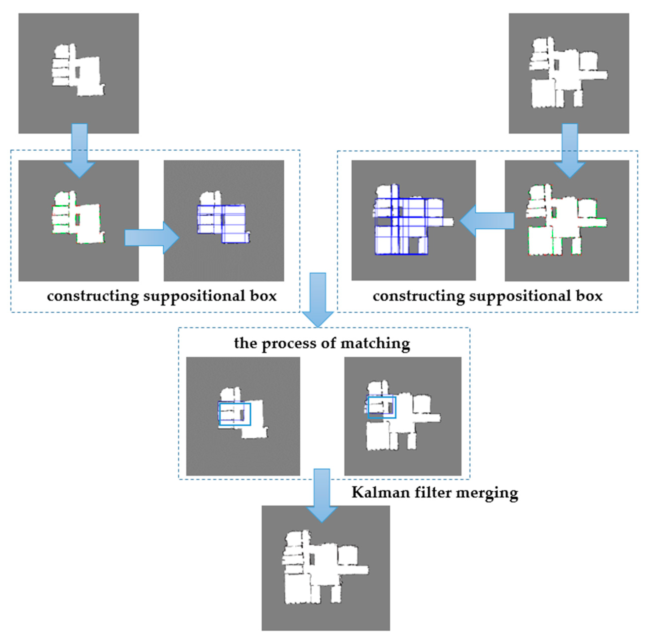
The matching features range from points to lines to other geometric features. Ferrao [14] used SIFT (Scale-Invariant Feature Transform) to calculate translation, rotation, and zoom between maps. However, according to their discussion, it was found that only matching feature points may not find the correct corresponding points. Therefore, reliability analysis is introduced on the basis of feature points [15]. Windows are built around the feature points, which can calculate the number of unknown state grids and filter mismatched feature points. Analogously, Jiang et al. [16] increased the precision by using MAFF (Map Augmentation and Feature Fusion). In addition, Tang et al. [17] combined SURF (Speeded Up Robust Features) features and RANSAC (RANdom Sample Consensus) algorithm as the initial value of the ICP (Iterative Closest Point) algorithm for map merging. Sun et al. [18] used Harris points to construct max common subgraph which is used as feature for map matching. In the grid map, each grid is represented by only three states after the threshold is divided. Thus, the description of the feature points is very similar, resulting in the point feature being unable to find the correct corresponding point. For lines matching, Carpin et al. [19] used the cross-correlation of the Hough spectrum to determine similar signals. After obtaining the rotation angle, they calculated the translation matrix through the X-spectrum and the Y-spectrum. On the basis of Hough spectrum, Lee et al. [20] enhanced this algorithm to improve the efficiency of the multi-robot system by identifying visual landmarks. Similarly, Sajad et al. [21] improved the accuracy by studying how to match the relative peak value correctly. Furthermore, Roh et al. [22] used Radon transform to extract the sinogram of the map. They took the coarse rotation matrix and translation matrix as the initial particle of the particle swarm algorithm to calculate the accurate value. However, it is easy to fall into a local maximum or minimum only by Radon transformation, so recently Lee [23] studied the Gaussian mixture model to optimize the transformation matrix on this basis. In addition to extracting existing lines from the map, some works [24,25] constructed lines based on scanning points. The difference is that the latter match based on the interconnections between the intersections of the two line segments. Although, in indoor grid maps, straight line features are very common, it takes a long time to match only with straight lines, which cannot meet the requirements of high efficiency. In the research based on geometric features, Adam et al. [26] proposed method based on wireframe mapping where the descriptor of each point is six variables and each edge is vectorized. Then, the weighted infinite norm between descriptors serves as a matching criterion. For some similar studies, Park et al. [27] proposed to construct the maximal empty rectangle in the map, so as to use the triangle position constraint between the empty rectangles to obtain the transformation relationship. Since the center of the empty rectangle will change due to the inconsistency of the map orthogonal coordinate system, the direction of the map orthogonal coordinate system needs to be unified. On the basis of that, Jazi [28] improves the orthogonal algorithm to speed up the matching speed, but the sensitivity of the empty rectangle to the rotated map still increases the complexity of the matching process. Our methods are not affected by this map rotation.

In addition to the above features extracted directly from the map, there are also some methods studying features fixed in the environment. Göksel et al. [29] find similar landmarks to match by identifying certain landmark information. Tsardoulias et al. [30] combined RFID (Radio Frequency Identification) positioning technology and ICP algorithm for grid map merging. However, the setting of feature points needs to be built in an unchanging environment, so the adaptability is not strong.

With the development of neural networks, some scholars use the features output from neural network to merge maps. Sajad et al. [31] used SOM neural network to conduct clustering feature for each segmented area, and the rotation angle is obtained by matching the norm vector histogram of the line connecting two cluster points and combining with Radon transform. Finally the x-y transformation was determined by using the norm vector of the matched cluster point. Although the number of feature output by the neural network is large in grid map, the mismatching is relatively high only according to these features. The other part was mainly based on the pose-graph map or topology map. Bonanni et al. [32] used the Voronoi diagram method to extract pose-graph map from grid map. They expanded the nodes from the existing pose-graph according to the breadth-first algorithm and optimize the expansion node by using the g2o libraries, and Lázaro et al. [33] directly merged topology map based on visual features (ORB features), then optimized the pose map using the g2o libraries. Similar to these works, other studies are focused on different optimization methods, likely feature filtering method [34] or RANSAC and Gauss–Newton method [35].

3. Method

The map merging method based on suppositional box is mainly divided into three steps: suppositional box construction, map matching based on suppositional box, and map merging.

3.1. The Construction of Suppositional Box

In our study, suppositional box is a virtual connection between four right-angled points which have position constraints. Generally, they have some commonalities. For instance, a suppositional box is composed of four right-angled points and two pairs of parallel sides. At the same time, four right-angled points have common edges between each other. Thus, it is easy to construct suppositional box by using common features, saying straight lines and right-angled points, in indoor environment. Hough transform [36] as a classics and mature method is used to detect straight lines in our research. Then the intersections of perpendicular straight lines are calculated as vertical points. Finally vertical points and perpendicular straight lines are grouped to construct suppositional box. Since these vertical points can also be intersecting points of straight line extension, the number of suppositional boxes extracted from the map is much, which can improve the success rate of matching.

3.1.1. Vertical Point Extraction

The vertical point is the intersection between perpendicular straight lines. Practically, a vertical point can represent the spatial vertical relationship between two objects. In other words, they can be either real connecting points or extension points of objects.

First, straight lines are detected in the grid map through Hough transform, and the slope and intercept of each straight line is calculated. Then, the slopes are used to find two perpendicular straight lines, that is, when two straight lines are perpendicular, the slopes of them are multiplied to −1. If two straight lines are in a perpendicular relationship, the intersection point of two straight lines is as the vertical point, as and ${\mathrm{p}}_2$ in Figure 2.

The vertical point is described by the coordinates of vertical point, the slope and intercept of two perpendicular straight lines constituting this vertical point. On the whole, the i-th vertical point descriptor is ${\mathrm{p}}_i$:

$${\mathrm{p}}_i=\left({\mathrm{vx}}_i{,\mathrm{vy}}_i{,\mathrm{k}}_{i1}{,\mathrm{b}}_{i1}{,\mathrm{k}}_{i2}{,\mathrm{b}}_{i2}\right) \times (i= 0,1\dots N)$$

(1)

where N is the number of vertical points. $\left({\mathrm{vx}}_i{,\mathrm{vy}}_i\right)$ is the vertical point coordinate value, ${\mathrm{k}}_{i1}$ and ${\mathrm{b}}_{i1}$ are the slope and intercept of one of the vertical sides respectively, ${\mathrm{k}}_{i2}$ and ${\mathrm{b}}_{i2}$ are the slope and intercept of the other vertical side, respectively. There is no requirement for the order of the two vertical sides. In the subsequent matching process, the slope and intercept of the two vertical sides will be used for matching.

3.1.2. Uncertainty Optimization of Vertical Points

Ideally, each vertical point is a unique representation in the map. However, the same wall sometimes is not made up of a straight line in grid map, because the state of each grid is calculated by probability. At the same time, a part of long wall will be recognized as several straight lines. Therefore, in the map, a vertical point in reality may be represented by a set of nearby points, as shown in Figure 3. In order to reduce the uncertainty, it is necessary to find an optimal one to represent these vertical points.

This paper uses clustering algorithm to group the vertical points that actually represent the same vertical point and find the optimal value to represent this set of vertical points. We take Euclidean distance as the goal to calculate the optimal coordinate, and defines it as an unconstrained optimization problem, as in Formula (2).

$$\left({\mathrm{vx}}_{\mathrm{best}}{,\mathrm{vy}}_{\mathrm{best}}\right)=\arg \min {{\displaystyle \sum _{m=0}^t\Vert \left({\mathrm{vx}}_m{,\mathrm{vy}}_m\right)-\left({\mathrm{vx}}_{\mathrm{best}}{,\mathrm{vy}}_{\mathrm{best}}\right)\Vert }}^2$$

(2)

where $\left({\mathrm{vx}}_{\mathrm{best}}{,\mathrm{vy}}_{\mathrm{best}}\right)$ is the optimal vertical point, $\left({\mathrm{vx}}_m{,\mathrm{vy}}_m\right)$ is the m-th vertical point in the same group, and t is the number of vertical points in the group. The optimization problem is solved by Newton method [37] which starts with any coordinate $({\mathrm{vx}}_0,{\mathrm{vy}}_0)$ selected within the group. The optimization precision is set as ε = $1\times {10}^{-8}$.

Some vertical points formed by the intersection of perpendicular extension straight line are not in the map outline. In order to improve the matching speed, these outliers are filtered using the neighborhood state difference method: a vertical point is taken as the starting point for four directions of diffusion; if there is no grid state different from this grid state in the four directions, then this vertical point is deleted.

3.1.3. Suppositional Box Building

In addition to the commonality of four right-angled points, suppositional box also has certain constraints on the positions of the four right-angled points. They must form a closed loop in the clockwise or counterclockwise direction. According to this constraint, suppositional box can be built by optimized vertical points.

Any vertical point can be chosen as the first right-angled point of suppositional box. A vertical side of this vertical point is selected as the target to find all other vertical points with the same slope and intercept which are the first candidate group. Then, a vertical point is randomly selected from above candidate object group as the second right-angled point of suppositional box, meanwhile the second candidate object group is obtained in the same way. Finally, the same method is used combined with the height and width distance constraints to find the fourth right-angled point of suppositional box. Repeat the above steps until all suppositional boxes that meet the requirements are extracted. When the fourth right-angled point is matched, in order to prevent the intersection of the sides of suppositional box, the height and width distance constraints are imposed. The process of building suppositional box is shown in Figure 4.

After each suppositional box is built, its descriptor can be defined by suppositional box’s height, width, area, center point, and vertical points as

$${\mathrm{R}}_q=({\mathrm{z}}_{q1}{,\mathrm{z}}_{q2}{,\mathrm{z}}_{q3}{,\mathrm{z}}_{q4},height,width,area,cx,cy)(q= 0,1\dots M)$$

(3)

where M is the number of suppositional box. ${\mathrm{R}}_q$ is the q-th suppositional box in the map, ${\mathrm{z}}_{q\mathrm{r}}=\left(x,y\right)$ is the coordinate of the r-th right-angled point in suppositional box, height is the long side of suppositional box, width is the short side of suppositional box, area is the area of suppositional box, (cx, cy) is the center point of suppositional box coordinate. Suppositional box matching will be based on this descriptor. See Algorithm 1 for the detailed process of suppositional box construction.

Algorithm 1 Suppositional box building

Input: the list of vertical points, ${\mathrm{p}}_i=\left({\mathrm{vx}}_i{,\mathrm{vy}}_i{,\mathrm{k}}_{i1}{,\mathrm{b}}_{i1}{,\mathrm{k}}_{i2}{,\mathrm{b}}_{i2}\right)$

Output: the list of suppositional box descriptor: ${\mathrm{R}}_q=({\mathrm{z}}_{q1}{,\mathrm{z}}_{q2}{,\mathrm{z}}_{q3}{,\mathrm{z}}_{q4},height,width,area,cx,cy)$

1: for $i$ = 1 → n do

2:  ${\mathrm{z}}_{q1}$ ← (${\mathrm{p}}_i$.vx, ${\mathrm{p}}_i$.vy)

3: ss ← True

4: while ss

5:   if $j_1$ = finding (${\mathrm{p}}_i$.$k_{i1}$,${\mathrm{p}}_i$.$b_{i1}$) //Find point with the same slope and intercept

6:     if $j_2$ = finding (${\mathrm{p}}_i$.$k_{i2}$,${\mathrm{p}}_i$.$b_{i2}$)//Find point with the same slope and intercept

7:       if $j_3$ = finding (${\mathrm{p}}_i$.$k_{i2}$,${\mathrm{p}}_i$.$b_{i2}$) and intersection ($i$,$j_1$,$j_2$,$j_3$)

// Find point that has the same slope and intercept and satisfies distance constraint constraint

8:            ${\mathrm{z}}_{q2}$ ←     (${\mathrm{p}}_{j1}$.vx, ${\mathrm{p}}_{j1}$.vy)

9:            ${\mathrm{z}}_{q3}$ ←     (${\mathrm{p}}_{j2}$.vx, ${\mathrm{p}}_{j2}$.vy)

10:            ${\mathrm{z}}_{q4}$ ←     (${\mathrm{p}}_{j3}$.vx, ${\mathrm{p}}_{j3}$.vy)

11:            height = max(dis(${\mathrm{z}}_{q1}$, ${\mathrm{z}}_{q2}$),dis(${\mathrm{z}}_{q2}$, ${\mathrm{z}}_{q3}$))//Define the long side to be height high

12:            width = min(dis(${\mathrm{z}}_{q1}$, ${\mathrm{z}}_{q2}$),dis(${\mathrm{z}}_{q2}$, ${\mathrm{z}}_{q3}$))//Define the short side to be width

13:            (cx, cy) = meancenter(${\mathrm{z}}_{q1}$,${\mathrm{z}}_{q2}$,${\mathrm{z}}_{q3}$,${\mathrm{z}}_{q4}$)//Compute the center point

14:            ${\mathrm{R}}_q$.append(${\mathrm{z}}_{q1}$,${\mathrm{z}}_{q2}$,${\mathrm{z}}_{q2}$, ${\mathrm{z}}_{q4}$,height, width, cx, cy)

15:             q ← q + 1

16:   else

17:       ss ←   False

18: end for

After building suppositional box circularly, right-angled points of each descriptor are randomly ordered. In order to reduce the time for subsequent matching, our method is designed to start from the lower left corner point and carry out counterclockwise sorting, generating a set of ordered right-angled points. As shown in Figure 5.

3.2. Suppositional Box Matching

On the whole, the process of matching is divided into two parts, rough matching, and filtration. It is important to note that the background of our work is based on the same resolution, only considering the translation and rotation of the map.

It is easy to match suppositional box by the side length. By default, the long side is height, and the short side is wide. Considering the error in the two-dimensional grid map established by the lidar, in order to match all the similar suppositional box pairs as much as possible, the threshold value is set to a larger number. Along with these a large number of pairs come the challenges of mismatching. Therefore, on the basis of rough matching with the side length, the process of filtering the mismatched pairs to obtain the optimal suppositional box pairs is proposed. In this study, the optimal suppositional box pairs can meet the alignment requirements of a large number of rough matching pairs and minimize the alignment error.

Through suppositional box matching, at least four pairs of corresponding right-angled points between two local maps can be directly found. The transformation matrix T can be calculated by the corresponding right-angled points, as shown in Equation (4).

$$\mathbf{T}=\left[\begin{array}{ccc}\cos \theta & -\sin \theta & t_x\\ \sin \theta & \cos \theta & t_y\\ 0& 0& 1\end{array}\right]$$

(4)

Firstly, a transformation matrix can be calculated for each rough match pair. Since the transformation matrix contains only three unknown variables, it can be calculated by three pairs of corresponding right-angled point pairs of suppositional box pairs. However, the arbitrarily sorted right-angled points of suppositional box descriptor means that the cyclic shift of point pairs must be considered in the computational process. Below we take two local maps ${\mathrm{map}}_1$ and ${\mathrm{map}}_2$ matching as an example. For any rough matching pair, select three points $\left({\mathrm{z}}_{11}{,\mathrm{z}}_{12}{,\mathrm{z}}_{13}\right)$ from suppositional box of ${\mathrm{map}}_1$ as the source point, correspondingly select $\left({\mathrm{z}}_{21}{,\mathrm{z}}_{22}{,\mathrm{z}}_{23}\right)$, $\left({\mathrm{z}}_{22}{,\mathrm{z}}_{23}{,\mathrm{z}}_{24}\right)$, $\left({\mathrm{z}}_{23}{,\mathrm{z}}_{24}{,\mathrm{z}}_{21}\right)$, $\left({\mathrm{z}}_{24}{,\mathrm{z}}_{21}{,\mathrm{z}}_{22}\right)$ from the corresponding suppositional box of ${\mathrm{map}}_2$ as candidate points. Now, 4 transformation matrixes ${\mathbf{T}}_0$, ${\mathbf{T}}_1$, ${\mathbf{T}}_2$ and ${\mathbf{T}}_3$ are obtained, respectively.

Secondly, it is the filtration process that try to remove incorrect match pairs. For the other suppositional box corresponding to ${\mathrm{map}}_1$ in the rough matching pair, we convert the coordinates of right-angled points to the ${\mathrm{map}}_2$ coordinate system by the transformation matrix ${\mathbf{T}}_0$. Then, the distance between four pairs of right-angled point is calculated. When the distance of the four right-angled points is less than a threshold, it is considered that this pair is successfully matched. Next, the number of successfully matched under the transformation ${\mathbf{T}}_0$ is counted. When the number of successful matching reaches the target value, ${\mathbf{T}}_0$ is considered a correct transformation matrix and put it into the candidate group. On the contrary, if the number is less than the threshold, then ${\mathbf{T}}_1$, ${\mathbf{T}}_2$, and ${\mathbf{T}}_3$ will be used to repeat the above process in turn.

Finally, score evaluation is used to obtain the optimal matching pair. After the aforementioned round of screening, transformation matrices can be calculated for the correctly matched pairs. They form a candidate group. In order to select the optimal transformation matrix from the candidate group, a scoring method is designed. The higher the score is, the smaller the alignment errors generated by the transformation matrix is. Based on this, a suppositional box pair with the highest score is selected as the optimal matching result. The score is mainly judged by the corresponding right-angled point distance and suppositional box area, see Equation (5). If the distance between the right-angled points of other suppositional box in the rough matching is smaller, the higher the accuracy of this pair is. Besides that, since the area of suppositional box is smaller, the area of the overlapping represented is smaller. These increase the error of other corresponding right-angled pairs. Therefore, the area is used as a reference factor. The smaller the pair area, the lower the weight.

$$S_{{\mathrm{R}}_1{\mathrm{R}}_2}=\frac{\min (\mathrm{area}\left({\mathrm{R}}_1\right),\mathrm{area}\left({\mathrm{R}}_2\right))}{{\displaystyle \sum _{\begin{array}{l}{\mathrm{R}}_1\in {\mathrm{map}}_1\\ {\mathrm{R}}_2\in {\mathrm{map}}_2\end{array}}\max ({\mathrm{d}}_{{\mathrm{R}}_1{\mathrm{R}}_{2}1},{\mathrm{d}}_{{\mathrm{R}}_1{\mathrm{R}}_{2}2},{\mathrm{d}}_{{\mathrm{R}}_1{\mathrm{R}}_{2}3},{\mathrm{d}}_{{\mathrm{R}}_1{\mathrm{R}}_{2}4})}}$$

(5)

where ${\mathrm{R}}_1$ and ${\mathrm{R}}_2$ are the matching suppositional box pairs, $\mathrm{area}\left({\mathrm{R}}_1\right)$ and $\mathrm{area}\left({\mathrm{R}}_2\right)$ are the corresponding suppositional box area, ${\mathrm{d}}_{{\mathrm{R}}_1{\mathrm{R}}_{2}1}$, ${\mathrm{d}}_{{\mathrm{R}}_1{\mathrm{R}}_{2}2}$, ${\mathrm{d}}_{{\mathrm{R}}_1{\mathrm{R}}_{2}3}$ and ${\mathrm{d}}_{{\mathrm{R}}_1{\mathrm{R}}_{2}4}$ are the Euclidean distance differences of the four corresponding right-angled points.

3.3. Map Merging

Local maps transformed to the same coordinate system by the optimal suppositional box pairs can be directly merged. However, it is evident that there are inconsistencies in the representation of the same region after map merging. For example, the same suppositional box does not align perfectly on the merged map. The reason is that there may be some errors in the optimal pairs. For reducing errors, Kalman filter is chosen.

In the process of grid map merging, we take the grid homogeneous coordinates as the state variable. The predictor variable is grid homogeneous coordinate $\hat{\mathbf{X}}$ of the coordinate system of ${\mathrm{map}}_2$, which is transformed from the corresponding grid homogeneous coordinates under the coordinate system of ${\mathrm{map}}_1$, and the observation variable $\hat{\mathbf{Z}}$ is represented as the same position in the ${\mathrm{map}}_2$.

Given any grid coordinates $\left(x,y\right)$ in ${\mathrm{map}}_1$, the predictor variable ${\hat{\mathbf{X}}}_n$ is calculated through the transformation matrix T.

$${\hat{\mathbf{X}}}_n={\left[x^{\prime },y^{\prime },1\right]}^{\mathrm{T}}=\mathbf{T}{\left[x,y,1\right]}^{\mathrm{T}}$$

(6)

where n = 0,1,2..., is the grid index. The transformation matrix obtained only by selecting three pairs of corresponding right-angled points of the matching pair may have some errors. Hence the prediction covariance matrix can be derived from the four transformation matrices ${\mathbf{T}}_{\mathrm{a}}$, ${\mathbf{T}}_{\mathrm{b}}$, ${\mathbf{T}}_{\mathrm{c}}$ and ${\mathbf{T}}_{\mathrm{d}}$ which are calculated by the cyclic combination of four sets of corresponding right-angled points of this pair.

First these four transformation matrices are used to find the corresponding four sets of homogeneous coordinate values, and then calculate the mean values in the x and y directions in turn:

$${\left[\overline{x},\overline{y},1\right]}^{\mathrm{T}}=\frac{1}{4}{\displaystyle \sum _{j=\mathrm{a}}^d{\mathbf{T}}_j}{\left[x^{\prime },y^{\prime },1\right]}^{\mathrm{T}}$$

(7)

Next, the predicted covariance matrix is calculated according to the above four sets of homogeneous coordinate values and mean values:

$${\mathbf{P}}_n=\left[\begin{array}{ccc}{\mathsf{\sigma }}_{\mathrm{x}}& 0& 0\\ 0& {\mathsf{\sigma }}_{\mathrm{y}}& 0\\ 0& 0& 1\end{array}\right],$$

(8)

where ${\mathsf{\sigma }}_{\mathrm{x}}={\displaystyle \sum _{s=0}^3\left(x^{\prime }{}_s-\overline{\mathrm{x}}\right)}$, ${\mathsf{\sigma }}_{\mathrm{y}}={\displaystyle \sum _{s=0}^3\left(y^{\prime }{}_s-\overline{\mathrm{y}}\right)}$

The matched optimal suppositional box pair is considered as the same area in environment; that is, the center points of its two suppositional boxes should theoretically be the same point in practice. Accordingly, the distance from the same grid point to the center point of the matched suppositional box in the two maps should be same. Thus, the observation value can be calculated by the distance from this point to the center point of the matched suppositional box:

$${\hat{\mathbf{Z}}}_n={\left[x^{″},y^{″},1\right]}^{\mathrm{T}},$$

(9)

$${\hat{\mathbf{Z}}}_n={\left[x^{″},y^{″},1\right]}^{\mathrm{T}},$$

(10)

$$y^{″}={\mathrm{y}}_{\mathrm{c}}{}_2+y^{\prime }-{\mathrm{y}}_{\mathrm{c}}{{}_1}^{\prime },$$

(11)

where $\left({\mathrm{x}}_{\mathrm{c}}{{}_1}^{\prime }{,\mathrm{y}}_{\mathrm{c}1}{}^{\prime }\right)$ is the center point coordinates value under the coordinate system of ${\mathrm{map}}_2$ transformed from the center point $\left({\mathrm{x}}_{\mathrm{c}1}{,\mathrm{y}}_{\mathrm{c}1}\right)$ of this suppositional box in ${\mathrm{map}}_1$, $\left({\mathrm{x}}_{\mathrm{c}2}{,\mathrm{y}}_{\mathrm{c}2}\right)$ is the corresponding center point of this suppositional box in ${\mathrm{map}}_2$.

Obviously, the error of center point comes from that the matching pairs are not exactly equal in length. Whereupon the observed error covariance matrix is calculated by the error value of height and width between the matching pair.

$${\mathbf{R}}_n=\left[\begin{array}{ccc}0.5\times △\mathrm{W}& 0& 0\\ 0& 0.5\times △\mathrm{H}& 0\\ 0& 0& 1\end{array}\right],$$

(12)

here, $△\mathrm{W}$ is the length error in the x direction, and $△\mathrm{H}$ is the length error in the y direction. 0.5 is the set parameter value.

Finally, the Kalman gain is calculated:

$${\mathbf{K}}_n={\mathbf{R}}_n/\left({\mathbf{R}}_n+{\mathbf{T}}_{\mathrm{a}}{\mathbf{P}}_n{\mathbf{T}}_{\mathrm{a}}{}^{\mathrm{T}}\right)$$

(13)

The Kalman estimate of grid coordinates is

$${{\hat{\mathbf{X}}}_n}^{\prime }={\mathbf{K}}_n{\hat{\mathbf{X}}}_n+\left(\mathbf{I}-{\mathbf{K}}_n\right){\hat{\mathbf{Z}}}_n,$$

(14)

Since the grid coordinates are integer values, the Kalman estimate result is finally rounded. During the process of merging, the state of grid in the two maps sometimes are different. The paper follows the following rules in

Table 1. The rules of grid’s state merging.

	S2	Occupancy	Free	Unknow
S1
occupancy		occupancy	occupancy	occupancy
free		occupancy	free	free
unknow		occupancy	free	unknow

S1 is the grid state value of this point in ${\mathrm{map}}_1$, S2 is the grid state value of this point in ${\mathrm{map}}_2$.

to determine the state of the grid.

4. Experimental Results and Analysis

In this section, we have verified our algorithm with various maps produced by simulation and real environment. In simulation experiments, the effectiveness of map merging method based on suppositional box is verified. Our method is also proved to be feasible in the case that the map orthogonal frame is inconsistent with the orthogonal frame of suppositional box. In a real environment, our method is performed under different indoor environment and proved of the higher rate of matching by comparing with other matching methods.

4.1. Experimental Verification under the Simulation Environment

In Ubuntu environment, we use Gazebo [38], a simulation software, to construct a simulation environment, as shown in Figure 6. In our implementation, the simulation robots equipped with lidar sensors construct two maps through the Gmapping [39] package in ROS. The Gmapping package can use the virtual lidar sensors to build a two-dimensional grid map based on the method of particle filtering. As the mapping area extending, the amount of data carried by particles will increase, resulting in an increase in the amount of calculation. However, compared with other mapping methods, it has a small computation cost and high accuracy in the small scenes.

The local maps, ${\mathrm{map}}_1$ and ${\mathrm{map}}_2$, are constructed by the two robots, respectively, as shown in Figure 7. By suppositional box matching algorithm, the optimal matching pair can be obtained. It can be seen that vertical points are not only the actual corner inflection points, but also the intersection points of some straight lines’ extension. Although we filter the vertical points that are not on the outline, some of them with different grid states around are reserved due to algorithm, which will not affect the matching process.

In following part, we demonstrate that Kalman filter can reduce the errors in the matching process of suppositional box. We use violent merging method and Kalman filter method respectively to carry out map merging experiment. The results are shown in Figure 8. Violent merging method is to merge the two maps directly. In Figure 8a, you can see that the same wall part appears twice, which is caused by the error of the transformation matrix. In Figure 8b, it clearly shows that the result is more consistent with the actual situation after optimization, which proves the effectiveness of Kalman filtering. In addition, according to statistics, the overlap contains a total of 22 edges, among which there are 9 non-coincident edges in violent merging method, and the sum of the length of non-coincident edges accounts for 31.6% of the sum of all the length of edges in the public area. In contrast, in the Kalman filter method, only one edge is not completely coincident, accounting for 2.4% of the total length.

In next part, we analyzed detailed errors in local map and merged map, respectively. The error is calculated by the differences of same objects between map and real environment.

The suppositional box is constructed on the basis of right-angled, which is component of the orthogonal frame. In the simulation environment, the orthogonal frame of suppositional box and map is usually in the same orientation. Actually, there will be certain differences between them. For example, in the real experiences, orthogonal frame of suppositional box may not coincide with orthogonal frame of map such as form a certain angle between them, which is a challenge for observed error in Kalman filter merging. As show in Figure 9. It is because that our method ignores the error caused by a certain angle between the orthogonal frame of them. Therefore, in order to comprehensively evaluate the performance of map merging method based on suppositional box, we test our method in scenes where the orthogonal frame of suppositional box and map is in the different orientation. In the test, the local map is rotated around the robot’s initial position point, so that the orthogonal frame of local map forms a certain angle with the orthogonal frame of suppositional box.

We selected eight walls characterized by a straight line in the overlapping area of the two local maps, as shown in Figure 10. We firstly record the actual length of the eight walls in Gazebo, then calculate the length of the eight walls in the two local maps and the merged map, respectively. The two local maps are ${\mathrm{map}}_1$ constructed by robot1 and ${\mathrm{map}}_2$ constructed by robot2. The length of the wall in map is calculated by the Euclidean distance between the pixel coordinates of the two ends of the wall multiplied by the resolution 0.05. Finally, the error results of the unrotated map, the 45° rotation map and the 90° rotation map are shown in

Table 2. The length error.

Wall’s Number	Actual Length (m)	$\mathbf{Error} \mathbf{in} {\mathbf{map}}_1$ (%)			$\mathbf{Error} \mathbf{in} {\mathbf{map}}_2$ (%)			Error in Merged Map (%)
		0°	45°	90°	0°	45°	90°	0°	45°	90°
1	6.25	0.00	2.40	0.00	2.40	1.60	0.80	1.60	1.60	1.60
2	1.25	8.00	0.80	0.00	0.00	4.00	4.00	4.00	1.60	0.00
3	5.25	4.76	2.85	0.95	1.90	2.28	2.85	0.90	1.71	0.00
4	3.25	7.69	7.38	8.33	7.69	9.84	9.23	0.00	8.61	9.23
5	3.25	10.77	9.84	9.23	15.38	8.61	9.23	7.60	7.69	4.61
6	1.50	12.00	8.00	10.67	7.33	8.00	12.00	8.70	6.00	7.33
7	2.50	4.00	6.80	6.00	6.00	5.20	6.00	6.00	3.60	8.00
8	7.50	2.00	2.40	2.00	2.67	2.40	2.00	1.30	0.93	1.33

.

From the above error data, we can see that the error of the merged map is mostly below the errors of local maps, and sometimes it is between them. First of all, the length of the wall in the merged map is very consistent with the actual length, and the average error is about 4%, indicating that our method is still feasible in the rotated map merging. Secondly, the superiority of multi-robot mapping can be proved because the merging method can reduce the accumulated errors of single-robot mapping over a long period of time.

Other rotated angle values in (0°, 360°) are randomly experimented to further illustrate the merging performance. The error results are shown in Figure 11. On the whole, the error of the merged map is about 4%, showing that the merged map is accord with the actual environment. From the analysis of different rotation angles, it can be seen that when the rotation angle is small, the error of the map does not change much. In the case of a large rotation angle, the error in local map increases due to the map rotation operation, and thus the error in merged map also increases. Even so, the error in merged map is still within 5%. In conclusion we can say, our proposed method based on suppositional box matching is not affected by map rotation.

4.2. Experimental Verification under the Real Environment

Here, we use two Fuxi cleaning robots to test our method. Each robot is equipped with a SICK-TIM561 single-line lidar, along with the Ubuntu 16.04 environment and ROS related function packages.

The real experiments are done in an office building in the Science Park of Central South University, as shown in Figure 12. The environment is mainly composed of corridors and connected rooms. Gmapping algorithm is used to build local maps of the environment.

The robots walk around in the environment and build two-dimensional grid maps. Taking into account the diversity of the environment, the robot builds four local maps in the real environment and divides them into two different groups for map merging. In Experiment 1, the robot explored a normal indoor environment with rooms in different directions. In Experiment 2, the robot explored a long corridor, which can construct multiple similar suppositional boxes. The experimental results are shown in Figure 13.

The advantage of the ubiquity and abundance of suppositional boxes in the environment may result in a high rate of false matches. However, from the above experimental results, it is obvious that the proposed method can be successfully applied in different environments, which proves our method can select the right one from a number of suppositional boxes.

To demonstrate the higher accuracy of the map merging method based on suppositional box, we compare it with the two feature point matching methods based on SURF [40] and ORB [41]. SURF and ORB feature have become the main research hotspots because of better speed and robustness for image matching compared with other feature points.

We selected two pairs of maps from the real indoor map dataset Halmstad–Robot-Maps [42]. This data set mainly collects environmental data of four different scenarios in Harmstad University. They used two methods to collect data, namely CAD drawing and sensor perception. The data set is mainly based on Google’s Tango Constructor application to build a three-dimensional grid map, and then select a certain horizontal plane to convert it into a two-dimensional grid map [43]. In the data set, a two-level map of the office lobby (E5 and F5) and two different residential apartment maps (HIH and KPT4A) are established. Among them, 14 two-dimensional grid maps are established in the E5 and F5 scene respectively, and there are 4 two-dimensional grid maps in the HIH and KPT4A scene, respectively. In the experiment, we select one pair of maps from the E5 scene as ${\mathrm{map}}_3$ and ${\mathrm{map}}_4$, and the other pair ${\mathrm{map}}_5$ and ${\mathrm{map}}_6$ from the F5 scene, as shown in Figure 14. The test is to count the number of correct matching features in different matching methods, and the result is shown in Figure 15. Our method, in terms of the number of suppositional boxes, is 17 and 15 pairs of features, respectively. However, transformation matrix is calculated on the basis of multiple pairs of corresponding feature points. Therefore, according to the number of matching feature points, the number of corresponding feature points obtained by our method is 68 and 60, respectively. In comparison, the number of corresponding feature points in our method far outweighs the other two methods. Importantly, the more the number of matching correct feature points, the higher the accuracy of the transformation matrix.

In general, the smaller the local environmental area explored by a single robot, the smaller the number of features in local map that can be extracted. Therefore, we divide the indoor map dataset into two categories according to area of local environment. Relatively speaking, in E5 and F5 scenes, the local environmental area explored by a single robot is large, while in HIH and KPTA4 scene, the local environmental area is small. We select four pairs of maps in E5 scene and three pairs of maps in the F5 scene. In HIH and KPT4A scene, one pair of maps were selected, respectively.

In addition to point features mentioned above, since Hough transform is used in our method, we choose another method based on Hough spectrum [19] for comparison. The performance of methods in terms of success rate is shown in

Table 3. The success rate comparison.

	E5 (%)	F5 (%)	HIH and KPT4A (%)
SURF + RANSAC	25.00	25.00	0.00
ORB + RANSAC	25.00	0.00	0.00
Hough spectrum	25.00	25.00	50.00
Our proposal	75.00	66.66	50.00

. From the result, we have a matching success rate of 75% and 66.66% in map groups with large area, whereas the ORB method has only 25% and 0%, the SURF method has 25% and 25%, meanwhile the method based on Hough spectrum only has 25% and 25%. Although we had only a 50% success rate in map groups with small area, none of the ORB method and SURF method matched successfully.

5. Conclusions

In this paper, we propose a map merging method based on suppositional box. Suppositional box is not only simple in structure, but also ubiquitous in indoor environment. This virtual structure feature can greatly facilitate the efficiency of map merging because a pair of suppositional boxes represents a pair of identical common area within which many other corresponding features can be extracted. What is more, it is not depend on the orientation of the map.

The main body of our approach is to find public areas based on suppositional box and merge map by Kalman filtering. Experimental results demonstrate its outperformance. We have shown, with experimental results, the merged map is more in line with the actual environment after reducing the errors of the optimal matching pairs. Further, compared with other matching method, a suppositional box pair can get more feature pairs like points or lines, which shows excellent matching abilities.

Despite the success of our approach, there are still challenging situations requiring additional research. Current research is only a simple violent fusion of three different grid states when facing with the different states fusion of same grid point. In fact, it is possible to discuss the probability weight of the grid based on the original probability grid. Therefore, in future research, it is expected that on the basis of this method, improvements can be made to the fusion of different grid state values, which can further improve the mapping accuracy.

References

1. Yu, S.; Fu, C.; Gostar, A.K.; Hu, M. A Review on Map-Merging Methods for Typical Map Types in Multiple-Ground-Robot SLAM Solutions. Sensors 2020, 20, 6988. [Google Scholar] [CrossRef]
2. Simmons, R.; Apfelbaum, D.; Burgard, W.; Fox, D.; Moors, M.; Thrun, S.; Younes, H. Coordination for Multi-Robot Exploration and Mapping; American Association for Artificial Intelligence: Monloparker, CA, USA, 2000. [Google Scholar]
3. Saeedi, S.; Trentini, M.; Li, H. A hybrid approach for multiple-robot SLAM with particle filtering. In Proceedings of the 2015 IEEE/RSJ International Conference on Intelligent Robots and Systems (IROS), Hamburg, Germany, 28 September–2 October 2015; pp. 3421–3426. [Google Scholar]
4. Howard, A. Multi-robot Simultaneous Localization and Mapping using Particle Filters. Int. J. Robot. Res. 2006, 25, 1243–1256. [Google Scholar] [CrossRef] [Green Version]
5. Sasaoka, T.; Kimoto, I.; Kishimoto, Y.; Takaba, K.; Nakashima, H. Multi-robot SLAM via Information Fusion Extended Kalman Filters. IFAC Pap. OnLine 2016, 49, 303–308. [Google Scholar] [CrossRef]
6. Zhou, X.S.; Roumeliotis, S.I. Multi-robot SLAM with Unknown Initial Correspondence: The Robot Rendezvous Case. In Proceedings of the 2006 IEEE/RSJ International Conference on Intelligent Robots and Systems, Beijing, China, 9–15 October 2006; pp. 1785–1792. [Google Scholar]
7. Xu, W.; Jiang, R.; Chen, Y. Map alignment based on PLICP algorithm for multi-robot SLAM. In Proceedings of the 2012 IEEE International Symposium on Industrial Electronics, Hangzhou, China, 28–31 May 2012. [Google Scholar] [CrossRef]
8. Lin, J.; Liao, Y.; Wang, Y.; Chen, Z.; Liang, B. A hybrid positioning method for multi-robot simultaneous location and mapping. In Proceedings of the Chinese Control Conference, Wuhan, China, 25–27 July 2018. [Google Scholar]
9. Lee, H.; Cho, Y.; Lee, B. Accurate map merging with virtual emphasis for multi-robot systems. Electron. Lett. 2013, 49, 932–934. [Google Scholar] [CrossRef]
10. Konolige, K.; Fox, D.; Limketkai, B.; Ko, J.; Stewart, B. Map merging for distributed robot navigation. In Proceedings of the 2003 IEEE/RSJ International Conference on Intelligent Robots and Systems (IROS 2003) (Cat. No.03CH37453), Las Vegas, NV, USA, 27–31 October 2003. [Google Scholar]
11. Carpin, S.; Andreas, B.; Viktoras, J. On map merging. Robot. Auton. Syst. 2005, 53, 1–14. [Google Scholar] [CrossRef]
12. Birk, A.; Carpin, S. Merging Occupancy Grid Maps From Multiple Robots. Proc. IEEE 2006, 94, 1384–1397. [Google Scholar] [CrossRef]
13. Ma, X.; Guo, R.; Li, Y.; Chen, W. Adaptive genetic algorithm for occupancy grid maps merging. In Proceedings of the 2008 7th World Congress on Intelligent Control and Automation, Chongqing, China, 25–27 June 2008. [Google Scholar] [CrossRef]
14. Ferrão, V.T.; Vinhal, C.D.N.; Da Cruz, G. An Occupancy Grid Map Merging Algorithm Invariant to Scale, Rotation and Translation. In Proceedings of the 2017 Brazilian Conference on Intelligent Systems (BRACIS), Uberlandia, Brazil, 2–5 October 2017; pp. 246–251. [Google Scholar]
15. Durdu, A.; Korkmaz, M. A novel map-merging technique for occupancy grid-based maps using multiple robots: A semantic approach. Turk. J. Electr. Eng. Comput. Sci. 2019, 27, 3980–3993. [Google Scholar] [CrossRef]
16. Jiang, Z.; Zhu, J.; Jin, C.; Xu, S.; Zhou, Y.; Pang, S. Simultaneously merging multi-robot grid maps at different resolutions. Multimed. Tools Appl. 2019, 1–20. [Google Scholar] [CrossRef]
17. Tang, H.; Sun, W.; Yang, K.; Lin, A.; Lv, Y.; Cheng, X. Grid map merging approach of multi-robot based on SURF feature. J. Electron. Meas. Instrum. 2017, 31, 859–868. [Google Scholar]
18. Yong, S.; Rongchuan, S.; Shumei, Y.; Yan, P. A Grid Map Fusion Algorithm Based on Maximum Common Subgraph. In Proceedings of the 13th World Congress on Intelligent Control and Automation, Changsha, China, 4–8 July 2018. [Google Scholar]
19. Carpin, S. Fast and accurate map merging for multi-robot systems. Auton. Robot. 2008, 25, 305–316. [Google Scholar] [CrossRef]
20. Lee, H.-C.; Lee, B.-H. Enhanced-spectrum-based map merging for multi-robot systems. Adv. Robot. 2013, 27, 1285–1300. [Google Scholar] [CrossRef]
21. Sajad, S.; Liam, P.; Michael, T.; Mae, S.; Howard, L. Map merging for multiple robots using Hough peak matching. In Proceedings of the IEEE/RSJ International Conference on Intelligent Robots and Systems, Vilamoura, Algarve, Portugal, 7–12 October 2012. [Google Scholar]
22. Roh, B.; Lee, H.C.; Lee, B.H. Multi-hypothesis map merging with sinogram-based PSO for multi-robot systems. Electron. Lett. 2016, 52, 1213–1214. [Google Scholar]
23. Lee, H. Tomographic Feature-Based Map Merging for Multi-Robot Systems. Electronics 2020, 9, 107. [Google Scholar] [CrossRef] [Green Version]
24. Lakaemper, R.; Latecki, L.; Wolter, D. Incremental multi-robot mapping. In Proceedings of the 2005 IEEE/RSJ International Conference on Intelligent Robots and Systems, Edmonton, AB, Canada, 2–6 August 2005; pp. 3846–3851. [Google Scholar]
25. Jafri, S.R.U.N.; Li, Z.; Chandio, A.A.; Chellali, R. Laser only feature based multi robot SLAM. In Proceedings of the 2012 12th International Conference on Control Automation Robotics & Vision (ICARCV), Guangzhou, China, 5–7 December 2012; pp. 1012–1017. [Google Scholar]
26. Caccavale, A.; Schwager, M. Wireframe Mapping for Resource-Constrained Robots. In Proceedings of the 2018 IEEE/RSJ International Conference on Intelligent Robots and Systems (IROS), Madrid, Spain, 1–5 October 2018; pp. 1–9. [Google Scholar]
27. Park, J.; Sinclair, A.J.; Sherrill, R.E.; Doucette, E.A.; Curtis, J.W. Map merging of rotated, corrupted, and different scale maps using rectangular features. In Proceedings of the 2016 IEEE/ION Position, Location and Navigation Symposium (PLANS), Savannah, GA, USA, 11–14 April 2016; pp. 535–543. [Google Scholar]
28. Jazi, S.H. Map-merging using maximal empty rectangles in a multi-robot SLAM process. J. Mech. Sci. Technol. 2020, 34, 2573–2583. [Google Scholar] [CrossRef]
29. Göksel, D.; Sukhatme, G.S. Landmark-based Matching Algorithm for Cooperative Mapping by Autonomous Robots. In Distributed Autonomous Robotic Systems 4; Parker, L.E., Bekey, G., Barhen, J., Eds.; Springer: Tokyo, Japan, 2000; pp. 251–260. [Google Scholar]
30. Tsardoulias, E.; Thallas, A.; Petrou, L. Metric map merging using RFID tags & topological information. arXiv 2017, arXiv:1711.06591. [Google Scholar]
31. Saeedi, S.; Paull, L.; Trentini, M.; Li, H. Neural network-based multiple robot Simultaneous Localization and Mapping. In Proceedings of the 2011 IEEE/RSJ International Conference on Intelligent Robots and Systems, Francisco, GA, USA, 25–30 September 2011; pp. 880–885. [Google Scholar] [CrossRef]
32. Bonanni, T.M.; Grisetti, G.; Iocchi, L. Merging Partially Consistent Maps. In Simulation, Modeling, and Programming for Autonomous Robots; Brugali, D., Broenink, J.F., Kroeger, T., MacDonald, B.A., Eds.; Springer: Cham, Germany, 2014; Volume 8810, pp. 352–363. [Google Scholar]
33. Lazaro, M.T.; Paz, L.M.; Pinies, P.; Castellanos, J.A.; Grisetti, G. Multi-robot SLAM using condensed measurements. In Proceedings of the 2013 IEEE/RSJ International Conference on Intelligent Robots and Systems, Tokyo, Japan, 3–7 November 2013; IEEE: Piscataway, NJ, USA, 2013. [Google Scholar] [CrossRef]
34. Deutsch, I.; Liu, M.; Siegwart, R. A framework for multi-robot pose graph SLAM. In Proceedings of the 2016 IEEE International Conference on Real-Time Computing and Robotics (RCAR), Angkor Wat, Cambodia, 6–10 June 2016; pp. 567–572. [Google Scholar]
35. Chen, H.; Huang, H.; Qin, Y.; Li, Y.; Liu, Y. Vision and laser fused SLAM in indoor environments with multi-robot system. Assem. Autom. 2019, 39, 297–307. [Google Scholar] [CrossRef]
36. Duda, R.O.; Hart, P.E. Use of the Hough transformation to detect lines and curves in pictures. Commun. ACM 1972, 15, 11–15. [Google Scholar] [CrossRef]
37. Qi, L.; Jie, S. A nonsmooth version of Newton’s method. Math. Program. 1993, 58, 353–367. [Google Scholar] [CrossRef]
38. Anderson, T.; Uffner, M.; Vogler, M.R.; Donnelly, B.C. Gazebo Structure. U.S. Patent No. 7,963,072, 21 June 2011. [Google Scholar]
39. Abdulgalil, M.A.; Nasr, M.M.; Elalfy, M.H.; Khamis, A.; Karray, F. Multi-robot SLAM: An Overview and Quantitative Evaluation of MRGS ROS Framework for MR-SLAM. In Advances in Human Factors, Business Management, Training and Education; Metzler, J.B., Ed.; Springer: Berlin/Heidelberg, Germany, 2018; Volume 751, pp. 165–183. [Google Scholar]
40. Bay, H.; Ess, A.; Tuytelaars, T.; Van Gool, L. Speeded-Up Robust Features (SURF). Comput. Vis. Image Underst. 2008, 110, 346–359. [Google Scholar] [CrossRef]
41. Rublee, E.; Rabaud, V.; Konolige, K.; Bradski, G. ORB: An efficient alternative to SIFT or SURF. In Proceedings of the IEEE International Conference on Computer Vision, Barcelona, Spain, 6–13 November 2011. [Google Scholar]
42. Halmstad-Robot-Maps. Available online: https://github.com/saeedghsh/Halmstad-Robot-Maps/ (accessed on 29 March 2021).
43. Shahbandi, S.G.; Magnusson, M. 2D map alignment with region decomposition. Auton. Robot. 2018, 43, 1117–1136. [Google Scholar] [CrossRef] [Green Version]
Figure 1. The framework of map merging method with suppositional box.
Electronics 10 00815 g001
Figure 2. Definition of the vertical point. Red circle is the vertical point. It indicates the intersection of two straight lines.
Electronics 10 00815 g002
Figure 3. Example of vertical points’ uncertainty. There are three walls in the map. The gray grid is the obstacle, the green line is the line identified by Hough transform, and the red point is the vertical point extracted by method mentioned in Section 3.1.1. The six vertical points on the left are intersection points of line features extracted from No. 1 wall and No. 2 wall. The four points on the right are intersection points of line features extracted from No. 2 wall and No. 3 wall.
Electronics 10 00815 g003
Figure 4. The process of building a suppositional box. (a) The gray point is the extracted vertical point, and the two straight lines are the direction of the vertical straight line. (b) The red point is a randomly selected vertical point; the red line is the target straight line direction. The blue point is the vertical point that matches the red line, forming candidate group one, as in (c). (d) Randomly select a point from candidate group one as the target circled in the figure, the blue line is the target straight line. The green point is the vertical point that matches the blue line, forming candidate group two. (e) Randomly select a point from the candidate group two as the target circled in the figure, there is no matching point. (f) Choose another point from the candidate group two. The green line is the target straight line, and the yellow point is the vertical point that matches the green line. (g) A suppositional box is formed by the constraint matching of length and width.
Electronics 10 00815 g004
Figure 5. Suppositional box building instance. Red rectangle is suppositional box extracted from map.
Electronics 10 00815 g005
Figure 6. Simulation environment.
Electronics 10 00815 g006
Figure 7. Suppositional box matching pair. (a) The map is built by robot1. (b) The map is built by robot2. The green line is the straight line recognized by Hough transform, the red point is the optimized vertical point, and the blue rectangle is suppositional box.
Electronics 10 00815 g007
Figure 8. The merging result. (a) is the result of violent merging method. (b) is the result of merging by Kalman filter.
Electronics 10 00815 g008
Figure 9. The case of inconsistent orthogonal frames. The top left is the orthogonal frame of map, and the middle is the orthogonal frameworks of suppositional box.
Electronics 10 00815 g009
Figure 10. Wall marked. ➀–➇ are the number of the selected wall.
Electronics 10 00815 g010
Figure 11. Analysis of mean error under different rotation angles.
Electronics 10 00815 g011
Figure 12. Real environment. (a) The Fuxi cleaning robot. (b) Two robots are exploring the corridor. (c) Two robots are exploring different rooms.
Electronics 10 00815 g012
Figure 13. Matching and merging results in real environment. (a,b) is the local map of Experiment 1, where have symmetrical room, (c) is the merged map of Experiment 1. (d,e) is the local map of Experiment 2, (f) is the merged map of Experiment 2.
Electronics 10 00815 g013
Figure 14. Map data pair. (a,b) The maps are selected from the E5 scene. (c,d) The maps are selected from the F5 scene.
Electronics 10 00815 g014
Figure 15. The number of correct matching feature point in different algorithms.
Electronics 10 00815 g015