The Possibility of Enhanced Power Transfer in a Multi-Terminal Power System through Simultaneous AC–DC Power Transmission

Abstract

The feasibility of power transfer enhancement, through simultaneous AC–DC power transmission in a two-terminal transmission network, has been proposed earlier by the authors, and the concept is well established. To meet the increase in demand for electricity, a new technique is proposed in this article to increase the use of existing transmission lines in addition to independent control of AC and DC power flow. This paper extends the concept to a three-terminal transmission network by considering a power tapping from the middle of the line. DC is also superimposed in the already existing three-terminal AC transmission system. In the proposed topology, a multi-terminal simultaneous AC–DC system is used, which is integrated with a zig-zag transformer and more than two voltage source converter (VSC) stations. Each terminal may represent an area of the power system. Anyone/two-terminal(s) may act as sending end, whereas the remaining two/one terminal(s) may act as receiving end. Power can flow in either direction through each segment of the transmission system. At sending end, VSC converts a part of AC to DC and injects it into the neutral of the zig-zag transformer. On receiving terminal, DC power is tapped from neutral of zig-zag transformer and fed to VSC for conversion back to AC. The concept is verified in the digital simulation software PSCAD/EMTDC.

1. Introduction

The maximum power transmission through the existing long AC transmission lines is restricted due to stability considerations, as it is not possible to load long extra-high voltage (EHV) AC transmission lines to their thermal limits to maintain a necessary stability margin [1,2,3]. Flexible alternating current transmission system (FACTS) devices are also used in the power transmission system to improve power transfer capacity and reliability. Presently, the majority of long transmission systems are AC, and for very long point-to-point bulk power transmission, a high-voltage direct current (HVDC) transmission system is suggested. HVDC is used on account of its low resistive losses. Initially, the commercial high voltage DC power transmission was developed for submarines. Nowadays, it is being adopted in long transmission lines to reduce transmission losses and also for back-to-back interconnection of asynchronous power grids [3,4,5]. Nevertheless, classical HDVC has several limitations. An active network is required at both ends, as it is incapable of reversing the direction of current flow and utilization of reactive power at both terminals, etc. [6,7]. The development of voltage source converter for high-voltage, direct current (VSC–HVDC) has helped to remove most of the difficulties of conventional HVDC and led to open new possibilities and new areas of applications [7]. This state-of-the-art technology comprises a three-phase switch-mode converter that employs pulse width modulation for voltage regulation.

A major attractive feature of VSC–HVDC is that it does not require changing the polarity of DC voltage for power flow in either direction. Apart from that, independent control of active and reactive power flow is possible [8,9]. Thus, VSC–HVDC is a capable system for developing a multi-Terminal HVDC transmission system [10,11,12,13,14].

The simultaneous AC–DC power transmission is an innovative concept that increases the stability and load-carrying ability of an existing long EHV AC transmission line [2]. The simultaneous AC–DC power realizes the advantage of HVDC in parallel with EHV AC transmission to improve system stability. In the proposed scheme, enhancement of power transfer without revising the existing EHV AC line is also possible. The principal benefits of this scheme are that the power transfer capacity of the line is improved remarkably, and the transient stability of the system is boosted up [15,16,17,18].

This paper introduces a three-terminal, simultaneous AC–DC power transmission system to enhance the power transfer capability of the line in addition to independent control of AC and DC power. This results in the economic operation of the system. The proposed control scheme used three zig-zag transformers, instead of a standard transformer and three VSCs, for making three-terminal, simultaneous AC–DC power transmission models. The function of one of the converters was to regulate DC voltage. The other two converters controlled the active power flow independently in either direction. With the use of zig-zag connected winding, a saturation of the transformer due to the flow of DC could be avoided. The windings of the zig-zag transformers were connected in such a way that the flux generated by the DC current flowing through each winding of the core of the zig-zag transformer was of equal magnitude and opposite in direction, thus canceling each other out so that the net continuous flux became zero. As a result, the core saturation due to the DC current was eliminated. Figure 1a shows the zig-zag connection of the transformer. A block diagram of a three-terminal, simultaneous AC–DC transmission model is shown in Figure 1b.

The operation of the proposed system was investigated for two cases; in the first case, all three power system areas had three-phase AC sources, and the output of the converters was synchronized to AC sources in their respective areas, whereas in the second case, two power system areas were connected to the AC source, and the other power system area was connected to the AC passive load. Digital simulation results conform to the theoretical concept and mathematical formulation of three-terminal, simultaneous AC–DC transmissions. Independent flow of AC power and DC power with independent power control were verified.

2. Control Strategy

In the proposed concept, AC and DC power could be transmitted from one power system area to two or more power system areas and vice versa. AC and DC power flowed independently with independent power control. AC power flow depended on the power angle (δ), whereas the DC power flow depended on VSC’s power settings. The control of VSC and the introduction of the proposed three-terminal, simultaneous AC–DC model are discussed in this section. The topology shown in Figure 1 is the same as traditional transmission links. The delta zig-zag-connected transformer is a key device in a simultaneous AC–DC system. The zig-zag-connected winding avoids saturation of the transformer produced by DC [2]. In addition, VSCs were included in each area. Control was achieved with outer and inner current controllers. The inner current controller depended on the currents involved in the VSC and a synchronous rotating frame of voltages. A phase-locked loop (PLL) controller determined the instantaneous phase and frequency [19,20,21].

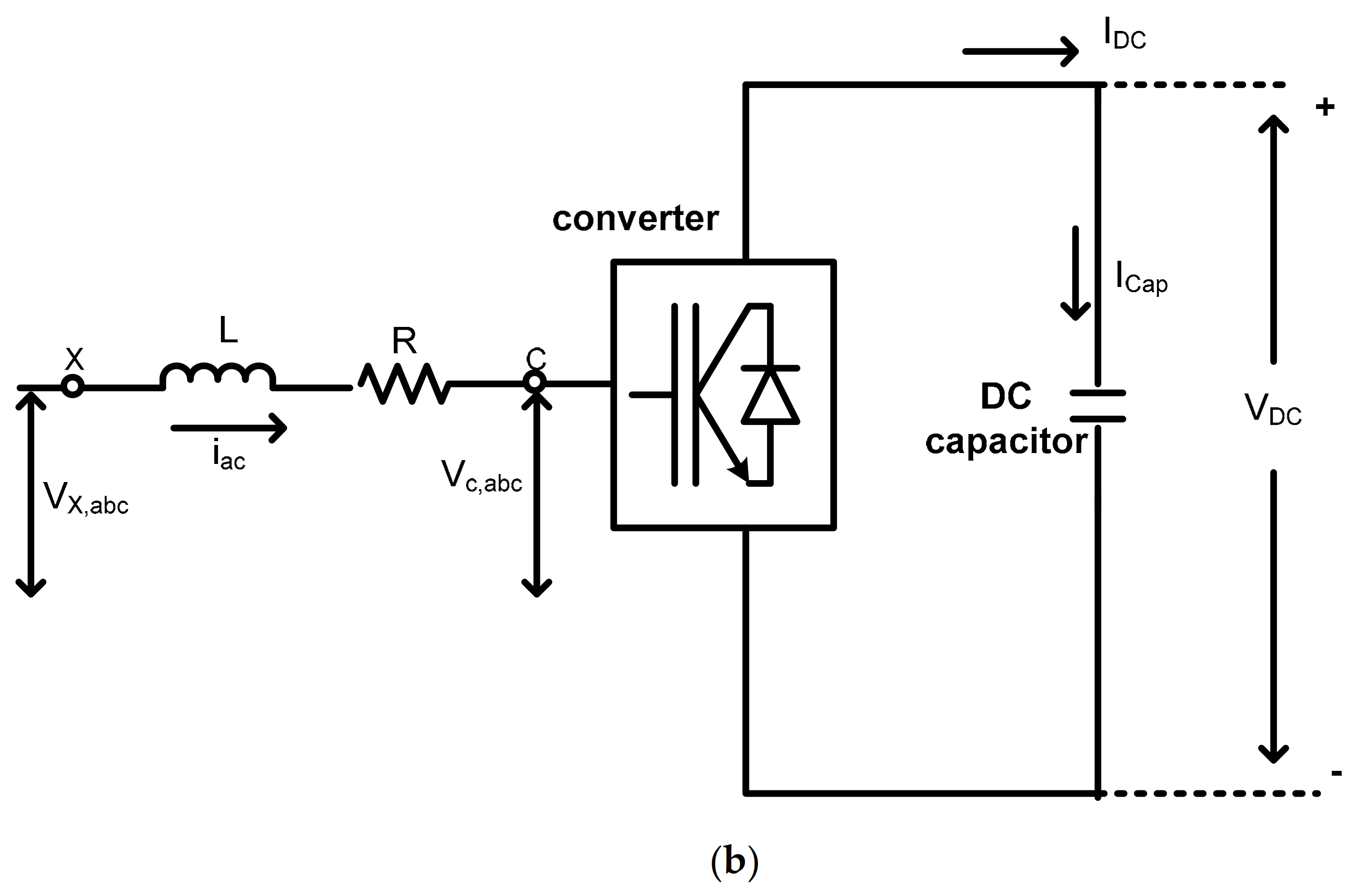
2.1. Equivalent Circuit of Voltage Source Converter

The schematic circuit of VSC is presented in Figure 2b, where R and L represent the total resistance and inductance coming out from the reactor and the transformer, respectively. The common coupling point of the AC system and VSC is indicated by X. Point C is the reference point for output voltages.

Applying KVL at the converter AC side in the abc reference frame, V can be expressed as

$${\mathrm{V}}_{\mathrm{x},\mathrm{abc}}-{\mathrm{V}}_{\mathrm{c},\mathrm{abc}}={\mathrm{Ri}}_{\mathrm{abc}}+\mathrm{L}\frac{{\mathrm{di}}_{\mathrm{abc}}}{\mathrm{dt}}$$

(1)

Applying abc-dq transformation to the above Equation (1) by Clark transformation,

$${\mathrm{V}}_{\mathrm{x},\mathsf{\alpha }\mathsf{\beta }}-{\mathrm{V}}_{\mathrm{c},\mathsf{\alpha }\mathsf{\beta }}={\mathrm{Ri}}_{\mathsf{\alpha }\mathsf{\beta }}+\mathrm{L}\frac{{\mathrm{di}}_{\mathsf{\alpha }\mathsf{\beta }}}{\mathrm{dt}}$$

(2)

$${\mathrm{V}}_{\mathrm{x},\mathsf{\alpha }\mathsf{\beta }}-{\mathrm{V}}_{\mathrm{c},\mathsf{\alpha }\mathsf{\beta }}={\mathrm{Ri}}_{\mathsf{\alpha }\mathsf{\beta }}+\mathrm{L}\frac{{\mathrm{di}}_{\mathsf{\alpha }\mathsf{\beta }}}{\mathrm{dt}}$$

(3)

From Parks transformation,

$${\mathrm{V}}_{\mathrm{x},\mathsf{\alpha }\mathsf{\beta }}={\mathrm{V}}_{\mathrm{x},\mathrm{dq}}{\mathrm{e}}^{\mathrm{j}\mathsf{\omega } \mathrm{t}}$$

(4)

$${\mathrm{V}}_{\mathrm{c},\mathsf{\alpha }\mathsf{\beta }}={\mathrm{V}}_{\mathrm{c},\mathrm{dq}}{\mathrm{e}}^{\mathrm{j}\mathsf{\omega } \mathrm{t}}$$

(5)

$${\mathrm{i}}_{\mathsf{\alpha }\mathsf{\beta }}={\mathrm{i}}_{\mathrm{dq}}{\mathrm{e}}^{\mathrm{j}\mathsf{\omega } \mathrm{t}}$$

(6)

Here, $\mathsf{\omega }$ is the fundamental angular frequency in the AC network. Substituting Equation (3) in Equation (2),

$${\mathrm{V}}_{\mathrm{x},\mathrm{dq}}{\mathrm{e}}^{\mathrm{j}\mathsf{\omega } \mathrm{t}}-{\mathrm{V}}_{\mathrm{c},\mathrm{dq}}{\mathrm{e}}^{\mathrm{j}\mathsf{\omega } \mathrm{t}}={\mathrm{Ri}}_{\mathrm{dq}}{\mathrm{e}}^{\mathrm{j}\mathsf{\omega } \mathrm{t}}+\mathrm{L}\frac{{\mathrm{di}}_{\mathrm{dq}}{\mathrm{e}}^{\mathrm{j}\mathsf{\omega } \mathrm{t}}}{\mathrm{dt}}$$

(7)

Dividing Equation (7) by ${\mathrm{e}}^{\mathrm{j}\mathsf{\omega } \mathrm{t}}$

$${\mathrm{V}}_{\mathrm{x},\mathrm{dq}}-{\mathrm{V}}_{\mathrm{c},\mathrm{dq}}={\mathrm{Ri}}_{\mathrm{dq}}+{\mathrm{j}\mathsf{\omega }\mathrm{Li}}_{\mathrm{dq}}+\mathrm{L}\frac{{\mathrm{di}}_{\mathrm{dq}}}{\mathrm{dt}}$$

(8)

Equation (8) can be written as

$$\frac{{\mathrm{di}}_{\mathrm{d}}}{\mathrm{dt}}=\frac{{\mathrm{V}}_{\mathrm{xd}}-{\mathrm{V}}_{\mathrm{cd}}}{\mathrm{L}}-\frac{{\mathrm{Ri}}_{\mathrm{d}}}{\mathrm{L}}-{\mathsf{\omega }\mathrm{i}}_{\mathrm{q}}$$

(9)

$$\frac{{\mathrm{di}}_{\mathrm{q}}}{\mathrm{dt}}=\frac{{\mathrm{V}}_{\mathrm{xq}}-{\mathrm{V}}_{\mathrm{cq}}}{\mathrm{L}}-\frac{{\mathrm{Ri}}_{\mathrm{q}}}{\mathrm{L}}+{\mathsf{\omega }\mathrm{i}}_{\mathrm{d}}$$

(10)

From Equations (9) and (10), the d, q axes equivalent circuits of the VSC seen from the AC network side is shown in Figure 3. The apparent power exchange observed from reference point X and in the d-q reference frame is given as

$${\mathrm{S}}_{\mathrm{dq}}=\frac{3}{2}{ \mathrm{V}}_{\mathrm{x},\mathrm{dq}}\ast {\mathrm{i}}_{\mathrm{dq}}^{*}=\frac{3}{2}\left({\mathrm{V}}_{\mathrm{xd}}+{\mathrm{jV}}_{\mathrm{xq}}\right)\left({\mathrm{i}}_{\mathrm{d}}-{\mathrm{ji}}_{\mathrm{q}}\right)$$

(11)

$${\mathrm{S}}_{\mathrm{dq}}=\frac{3}{2}\left({\mathrm{V}}_{\mathrm{xd}}{\mathrm{i}}_{\mathrm{d}}+{\mathrm{V}}_{\mathrm{xq}}{\mathrm{i}}_{\mathrm{q}}\right)+\mathrm{j}\left({\mathrm{V}}_{\mathrm{xq}}{\mathrm{i}}_{\mathrm{d}}-{\mathrm{V}}_{\mathrm{xd}}{\mathrm{i}}_{\mathrm{q}}\right)$$

(12)

In a steady state, active power exchange at point X will be equal to the power exchange at the DC bus.

$${\mathrm{P}}_{\mathrm{dq}}={\mathrm{P}}_{\mathrm{dc}}$$

(13)

$$\frac{3}{2}\left({\mathrm{V}}_{\mathrm{xd}}{\mathrm{i}}_{\mathrm{d}}+{\mathrm{V}}_{\mathrm{xq}}{\mathrm{i}}_{\mathrm{q}}\right)={\mathrm{V}}_{\mathrm{dc}}{\mathrm{I}}_{\mathrm{dc}}$$

(14)

Equation (14) can be rearranged, and hence, at a steady-state DC current becomes

$${\mathrm{I}}_{\mathrm{dc}}=\frac{{\mathrm{P}}_{\mathrm{dq}}}{{\mathrm{V}}_{\mathrm{dc}}}=\frac{3\left({\mathrm{V}}_{\mathrm{xd}}{\mathrm{i}}_{\mathrm{d}}+{\mathrm{V}}_{\mathrm{xq}}{\mathrm{i}}_{\mathrm{q}}\right)}{2{\mathrm{V}}_{\mathrm{dc}}}$$

(15)

2.2. Control of VSC Connected to Passive Network

VSC linked to the passive link has to maintain fixed phase voltages for all loads ranging from no load to full load [22,23]. The load impedance is taken as Z_L. V_c,rms is expressed as

$${\mathrm{V}}_{\mathrm{c},\mathrm{rms}}=\frac{m_a{V}_{dc}}{2\sqrt{2}}$$

(16)

Equation (17) gives the voltage across the load.

$${\mathrm{V}}_{\mathrm{x},\mathrm{rms}}=\frac{Z_L}{Z_L+\left(\mathrm{R}+\mathrm{j}\mathsf{\omega }\mathrm{L}\right)}{\mathrm{V}}_{\mathrm{c},\mathrm{rms}}=\frac{Z_L}{Z_L+\left(\mathrm{R}+\mathrm{j}\mathsf{\omega }\mathrm{L}\right)}\frac{m{V}_{dc}}{2\sqrt{2}}$$

(17)

Here, m is the output of the controller that is fed from the error signal in the reference and actual phase voltage.

2.3. VSC Control Connected to Active AC Network

In this case, the space vector approach enables decoupling the linear control of active and reactive currents. The reference frame d-q is selected such that the voltage of phase A is aligned with the d-axis at point X. This results in

$${\mathrm{V}}_{\mathrm{xq}}=0 \mathrm{and} {\mathrm{V}}_{\mathrm{xd}}={\mathrm{V}}_{\mathrm{x}}$$

(18)

Putting these voltage components in Figure 3 for the case of the alignment of d-axis aligned with phase A, the active and reactive power can be obtained as

$${\mathrm{P}}_{\mathrm{dq}}=\frac{3}{2}{\mathrm{V}}_{\mathrm{xd}}{\mathrm{i}}_{\mathrm{d}} \mathrm{and} {\mathrm{Q}}_{\mathrm{dq}}=\frac{-3}{2}{\mathrm{V}}_{\mathrm{xd}}{\mathrm{i}}_{\mathrm{q}}$$

(19)

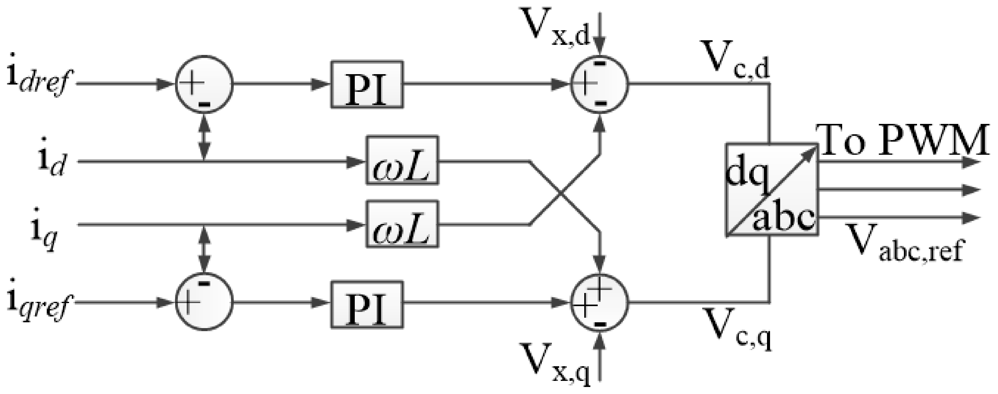
2.4. The Inner and Outer Current Controller

Based on Equations (9) and (10), an inner current controller is developed. The d and q-axis current controllers of the inner current loop are shown in Figure 4. The d and q-axis reference currents are set as i_dref and i_qref, respectively [20,24]. The active current id is used for the outer loop to control either DC voltage level or active power flow. The reactive current i_q is used to control either AC voltage support in weak grid connection or reactive power flow into stiff grid connection.

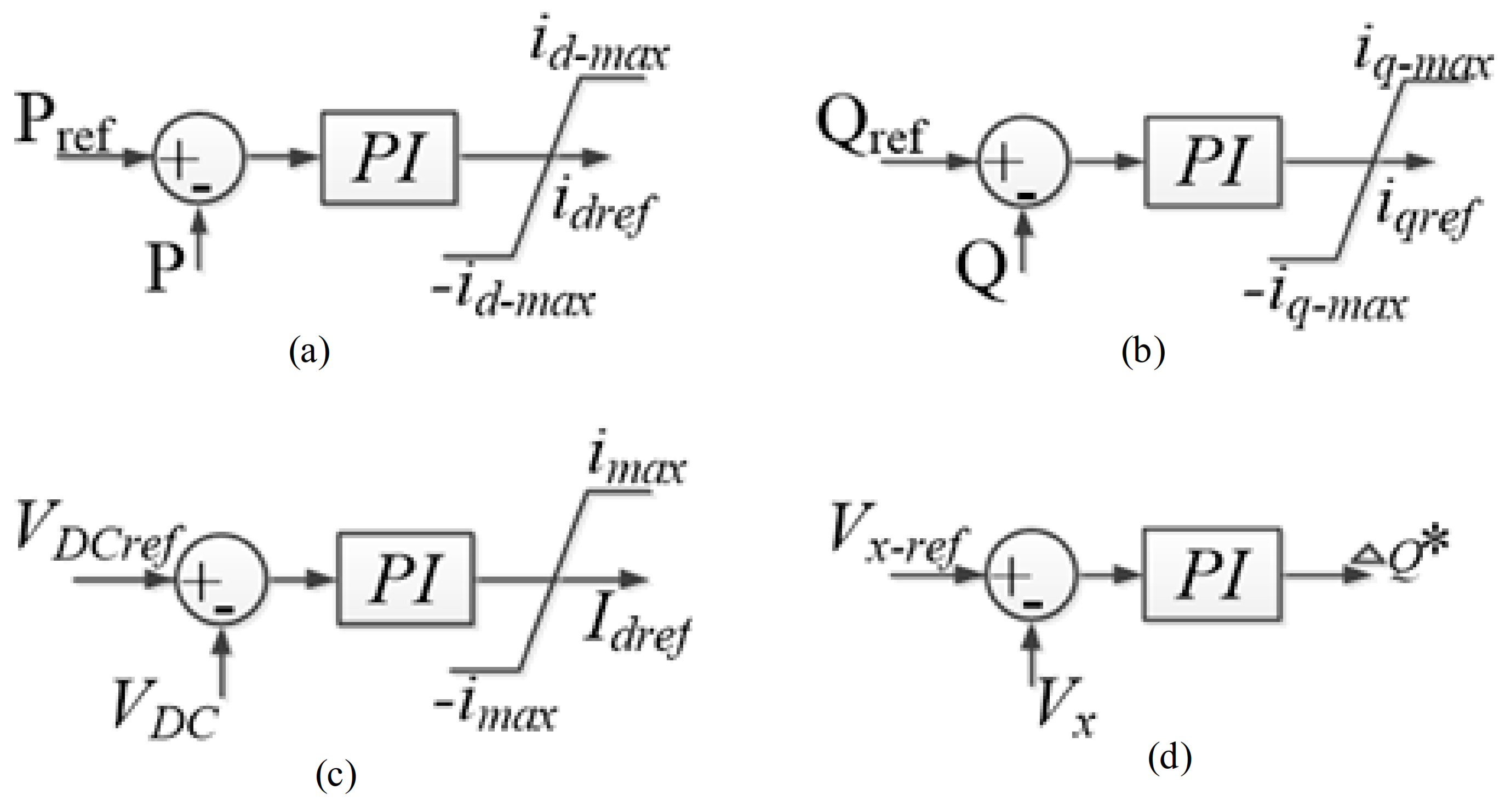
2.5. Active Power Control

From Equation (18), ${\mathrm{V}}_{\mathrm{xd}}={\mathrm{V}}_{\mathrm{x}},$ and from Equation (19), active power flow is given as ${\mathrm{P}}_{\mathrm{dq}}=\frac{3}{2}{\mathrm{V}}_{\mathrm{xd}}{\mathrm{i}}_{\mathrm{d}}$, where V_x is required to have a constant value. Therefore, active power flow is controlled by an active current i_d. The active power controller i_dref will be the reference input to the d-axis current controller of the inner current loop shown in Figure 5. A limiter is used to apply the limit on the output of the power controller, where ${\mathrm{i}}_{\mathrm{d}-\max }={\mathrm{i}}_{\mathrm{rated}}$

The reactive power is given by ${\mathrm{Q}}_{\mathrm{dq}}=\frac{-3}{2}{\mathrm{V}}_{\mathrm{xd}}{\mathrm{i}}_{\mathrm{q}}$ and is controlled by reactive current i_q. i_qref is limited to +/−Iq-max such that I_max= I_rated. Hence,

$${\mathrm{i}}_{\mathrm{q}\_\max }=\sqrt{{\mathrm{I}}_{\max }^{ 2}-{\mathrm{i}}_{\mathrm{dref}}^{ 2}}$$

(20)

2.6. DC and AC Voltage Control

Ignoring the converter losses, the energy balance equation of VSC can be written as

$${\mathrm{P}}_{\mathrm{ac}}+{ \mathrm{P}}_{\mathrm{dc}}+{\mathrm{P}}_{\mathrm{cap}}=0$$

(21)

$$\frac{3}{2}{\mathrm{V}}_{\mathrm{xd}}{\mathrm{i}}_{\mathrm{d}}+{ \mathrm{V}}_{\mathrm{dc}}{\mathrm{I}}_{\mathrm{dc}}+{\mathrm{V}}_{dc}{\mathrm{i}}_{\mathrm{cap}}=0$$

(22)

where i_cap and I_dc are the capacitor current and DC bus current, respectively. Capacitor current can be given as

$${\mathrm{i}}_{\mathrm{cap}}=-(\frac{3{\mathrm{V}}_{\mathrm{xd}}{\mathrm{i}}_{\mathrm{d}}}{2{\mathrm{V}}_{\mathrm{dc}}}+{\mathrm{I}}_{\mathrm{dc}}) \mathrm{and} {\mathrm{i}}_{\mathrm{cap}}=\mathrm{C}\frac{{\mathrm{dV}}_{dc}}{\mathrm{dt}}$$

(23)

From the above two equations, the DC voltage becomes

$$\frac{{\mathrm{dV}}_{dc}}{\mathrm{dt}}=-\frac{1}{\mathrm{C}}(\frac{3{\mathrm{V}}_{\mathrm{xd}}{\mathrm{i}}_{\mathrm{d}}}{2{\mathrm{V}}_{dc}}+{\mathrm{I}}_{\mathrm{dc}})$$

(24)

From the above equation, the DC voltage can be controlled by the active current (i_d).I_dc represents a feed-forward control. DC voltage is maintained constant with the help of PI controller. From Equation (1),

$$\frac{{\mathrm{dV}}_{dc}}{\mathrm{dt}}=-\frac{1}{\mathrm{C}}(\frac{3{\mathrm{V}}_{\mathrm{xd}}{\mathrm{i}}_{\mathrm{d}}}{2{\mathrm{V}}_{dc}}+{\mathrm{I}}_{\mathrm{dc}})$$

(25)

$${\mathrm{i}}_{\mathrm{abc}}={\left(\frac{\mathrm{s}}{\mathrm{v}}\right)}^{*}=\frac{\mathrm{P}-\mathrm{jQ}}{\mathrm{v}*}$$

(26)

If V_c,abc remains constant, and P is controlled at a certain value, then

$${\mathsf{\Delta }\mathrm{V}}_{\mathrm{x},\mathrm{abc}}=\frac{\mathsf{\omega }\mathrm{L}}{{\mathrm{V}}_{\mathrm{x},\mathrm{abc}}}\mathsf{\Delta }\mathrm{Q}$$

(27)

Thus, V_x,abc is maintained constant through reactive power compensation.

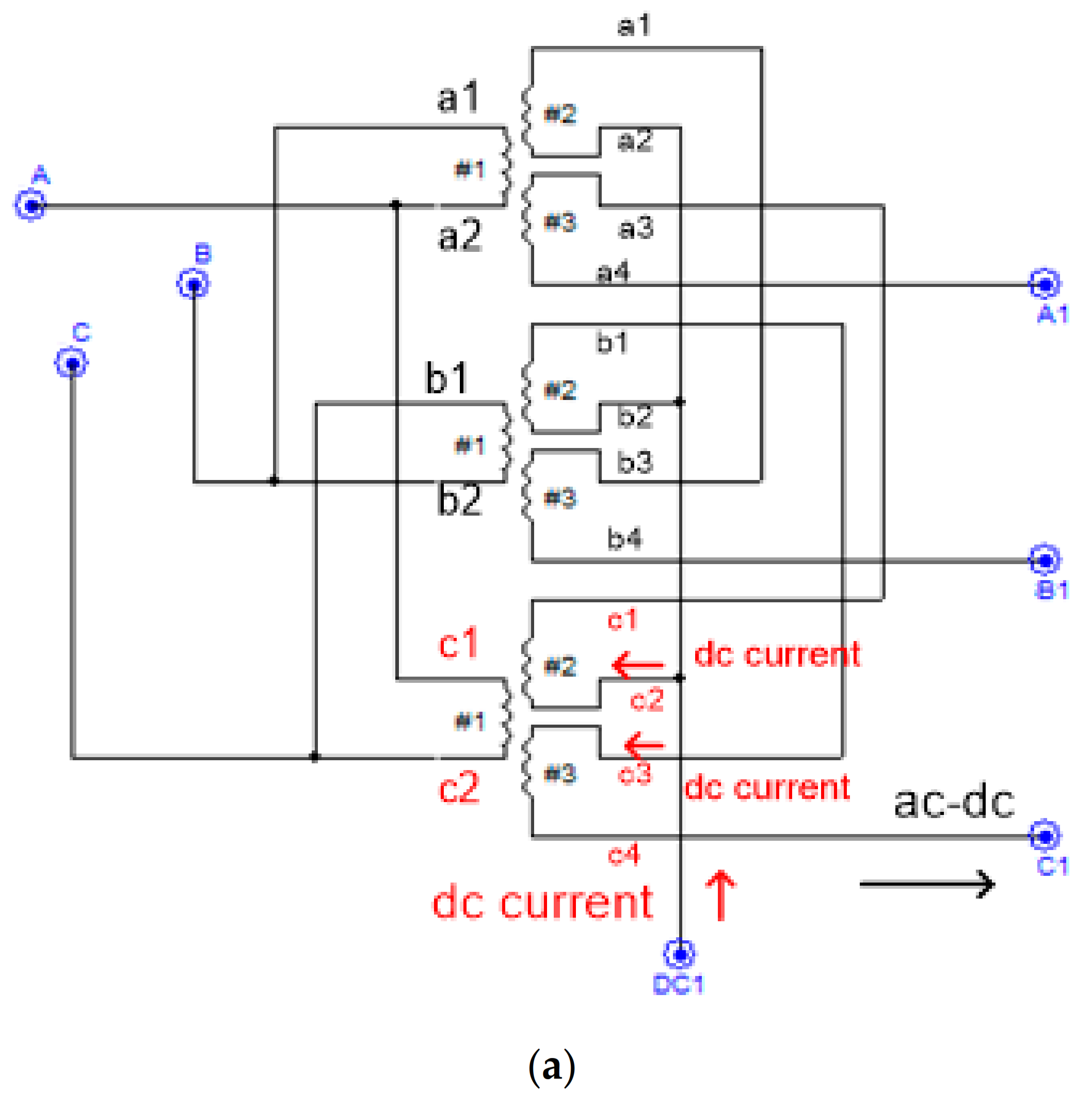
2.7. Simultaneous AC–DC System

The idea of a three-terminal, simultaneous AC–DC power transmission control strategy for VSC was discussed in the above sections. Some of the formulae for the transformation of the HVAC line to simultaneous AC–DC power transmission are discussed in this section. The active and reactive power of the converter is expressed in [2,25]. Based on these,

$${\mathrm{P}}_{\mathrm{dq}}=\frac{3}{2}{\mathrm{V}}_{\mathrm{xd}}{\mathrm{i}}_{\mathrm{d}}{ \mathrm{Q}}_{\mathrm{dq}}=\frac{-3}{2}{\mathrm{V}}_{\mathrm{xd}}{\mathrm{i}}_{\mathrm{q}}$$

(28)

The total rms current of each conductor is given as [2].

$$\mathrm{I}=\left[I_a^2+{\left(I_{dc}/3\right)}^2\right]{ }^{\raisebox{1ex}{$1$}\!\left/ \!\raisebox{-1ex}{$2$}\right.}$$

(29)

I_a is the rms AC current per conductor at any point of the line.

Now, the total current through the conductor equal to its thermal limit (I_th) is given by

$$I_{th}=\left[I_a^2+{\left(I_{dc}/3\right)}^2\right]{ }^{\raisebox{1ex}{$1$}\!\left/ \!\raisebox{-1ex}{$2$}\right.}$$

(30)

where V_ph is the per phase rms voltage of the original AC line, and V_a is the per phase voltage of AC component of simultaneous AC–DC line with DC voltage V_dc superimposed on it [2]. As insulators remain unchanged, the peak voltage in both cases should be equal.

$$V_{max}=\sqrt{2}{V}_{ph}=V_{dc}+\sqrt{2}{V}_a$$

(31)

Allowing maximum permissible voltage offset such that the simultaneous voltage wave just touches zero in each cycle [2],

$$V_{dc}=V_{ph}/\sqrt{2} \mathrm{and} V_a=V_{ph}/2$$

(32)

Total power transfer through the single circuit line before conversion is given as [2].

$$P^{\prime }\approx 3 V_{ph}^{ 2} \sin {\delta }_1/\mathrm{X}$$

(33)

where ${\delta }_1$ is the power angle, and X is the per phase transfer reactance. The value of ${\delta }_1$ may be obtained from the load curve by knowing the transfer reactance X of the line and the surge impedance loading.

$$P^{\prime }total=\mathrm{M}\ast \mathrm{SIL}$$

(34)

where M is the multiplying factor, and its magnitude decreases with the length of the line. The value of M can be obtained from the load–ability curve [2,26]. Power transfer through the simultaneous AC–DC system [2,26].

$$P_{total}=P_{ac}+P_{dc}=3V_a^2\sin {\delta }_2/X+V_{dc}{I}_{dc}$$

(35)

Here, in this case, the power angle ${\delta }_2$ between the AC voltages at the two ends of simultaneous AC–DC system can be enhanced to a very high value due to fast controllability of the DC power. Thus, from Equations (33) and (35),

Percentage power enhancement = {(P_total − P’) × 100}/P_total

(36)

Approximate value of AC current per phase [2]

$$I_a=V(\sin {\delta }_2/2)/X$$

(37)

DC current can be adjusted according to the thermal limit by

$${\mathrm{I}}_{\mathrm{dc}}=3\sqrt{{\mathrm{I}}_{\mathrm{th}}^{*2}-{\mathrm{I}}_{\mathrm{a}}^{*2}}$$

(38)

3. System under Study and Its Simulation Results

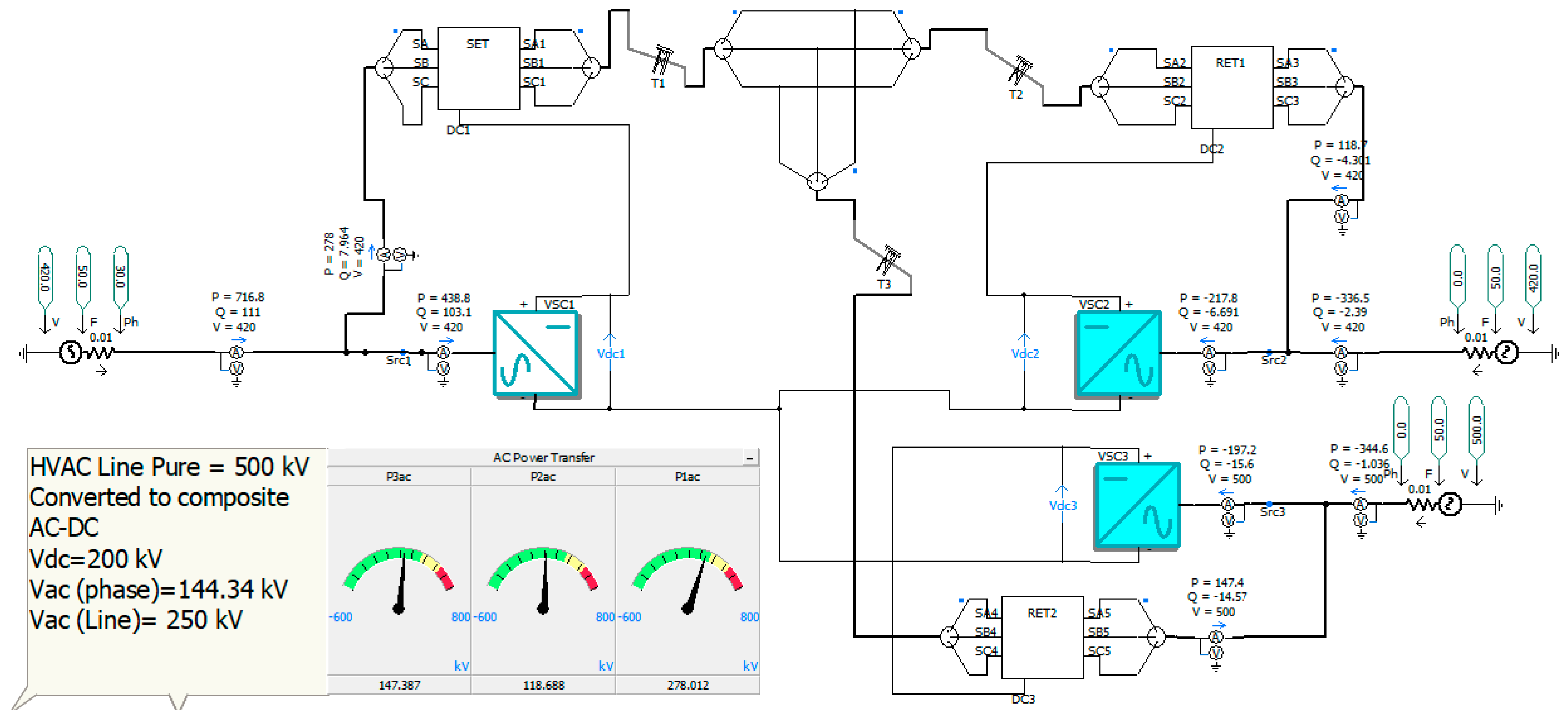
3.1. Multi-Terminal, Simultaneous AC–DC Power Transmission

Figure 1b depicts the three power system areas in which an AC network is connected through 500 kV and 500 km single circuit HVAC transmission lines. The same line was transformed to a simultaneous AC–DC line with 250 kV AC (144.34 kV phase voltage) with a DC voltage of 200 kV superimposed [2]. Area-1 consisted of an AC power source of 420 kV, delta-zig-zag transformer, and VSC1, which controlled DC voltage. Area-2 consisted of an AC power source of 420 kV, delta-zig-zag transformer, and VSC2, controlling the active power flow. Additionally, area-3 consisted of an AC power source of 500 kV, delta-zig-zag transformer, and VSC3 in active power control mode.

All three-phase VSCs were connected to their respective area AC network through converter transformer with appropriate turns ratio on the AC side. Their DC side positive terminals were connected to the neutral point of the zig-zag transformer present in their areas. Earth was taken as the return path for DC. Hence, the line conductors carried DC, which was superimposed on AC. Area 1 was connected to area-2 through a single-circuit transmission line of 500 km, which carried both AC and DC. In the middle of the transmission line at 250 km, tapping was performed to connect area-3 through the 250 km transmission line. Simultaneous AC–DC current flowed through the transmission lines. The converter and network system models were established and verified in digital simulation software PSCAD/EMTDC. To validate the possibility of multi-terminal, simultaneous AC–DC power transmission, two cases were considered.

Table 1. System data used for simulation.

	AC Side Data
	Area-1		Area-2	Area-3
AC voltage	420 kV		420 kV	500 kV
Frequency Delta-Zig-Zag Transformer	50 Hz 1000 MVA 420/250 kV		50 Hz 1000 MVA 420/250 kV	50 Hz 1000 MVA 500/250 kV
Converter Transformer	1000 MVA 420/115 kV		1000 MVA 420/115 kV	1000 MVA 500/115 kV
	Simultaneous AC–DC Transmission Line Parameters
	Length	R (ohms/m)	XL (ohms/m)	XC (mohms/m)
VSC1 to VSC2	500 km	0.3252 × 10−4	0.33086 × 10−3	295.88
VSC1 to VSC3	500 km	0.3252 × 10−4	0.33086 × 10−3	295.88
DC side capacitor: 300 µF; DC voltage: 200 kV; Line-line AC voltage of VSC: 115 kV

shows system simulation data.

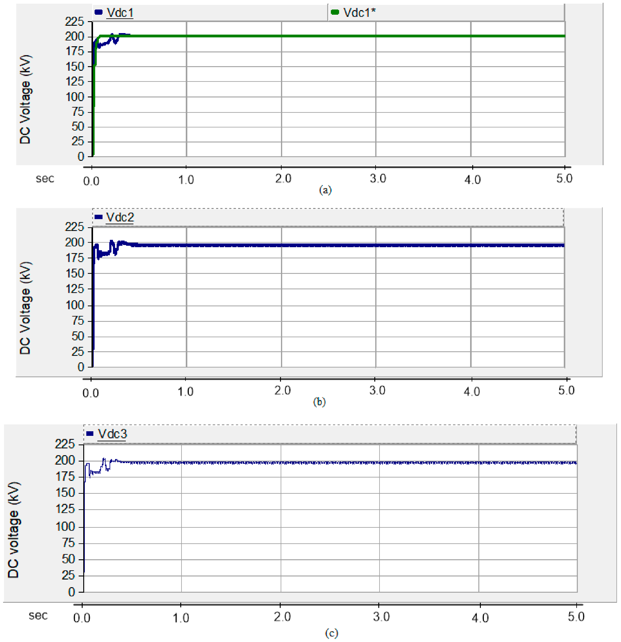
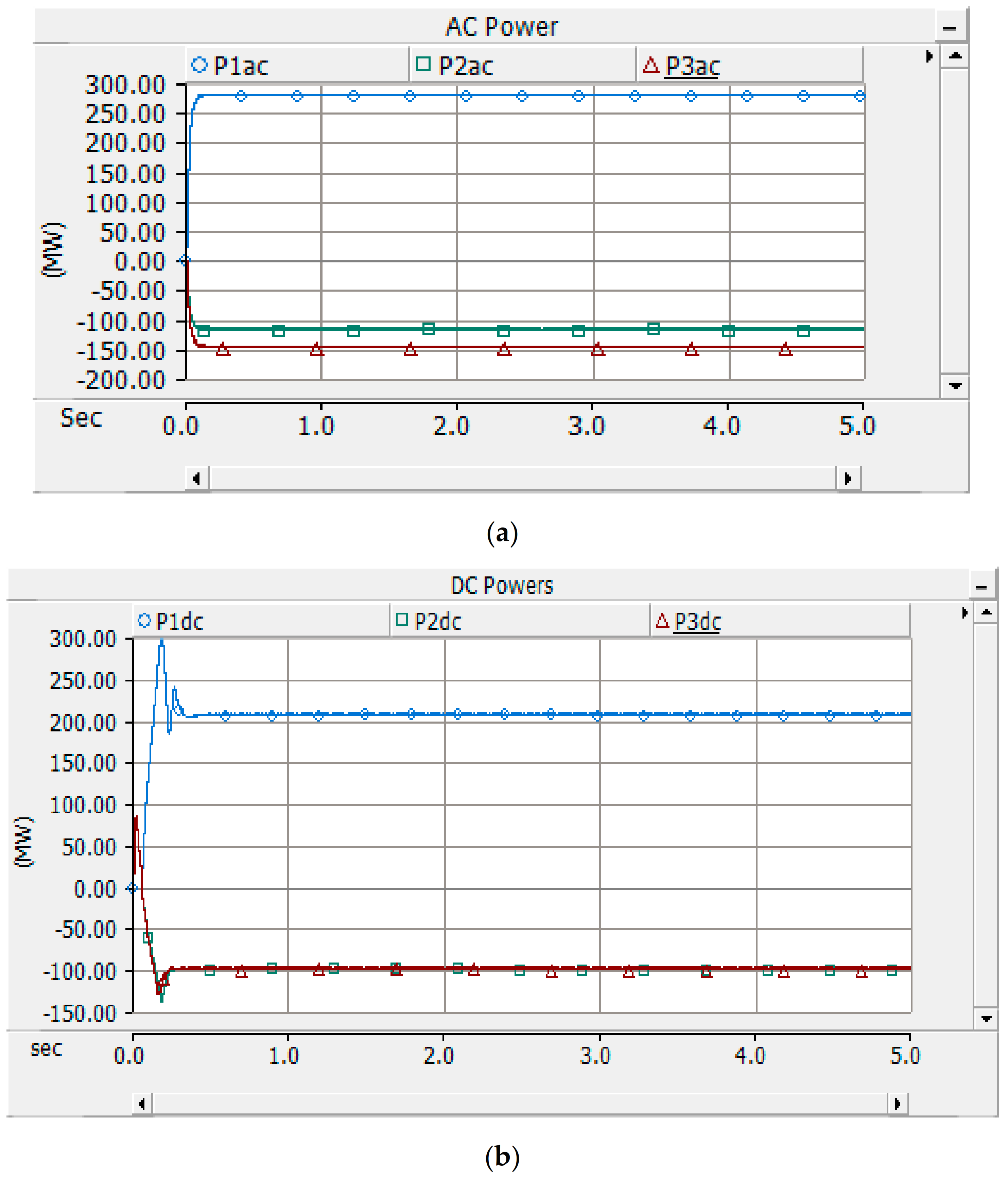
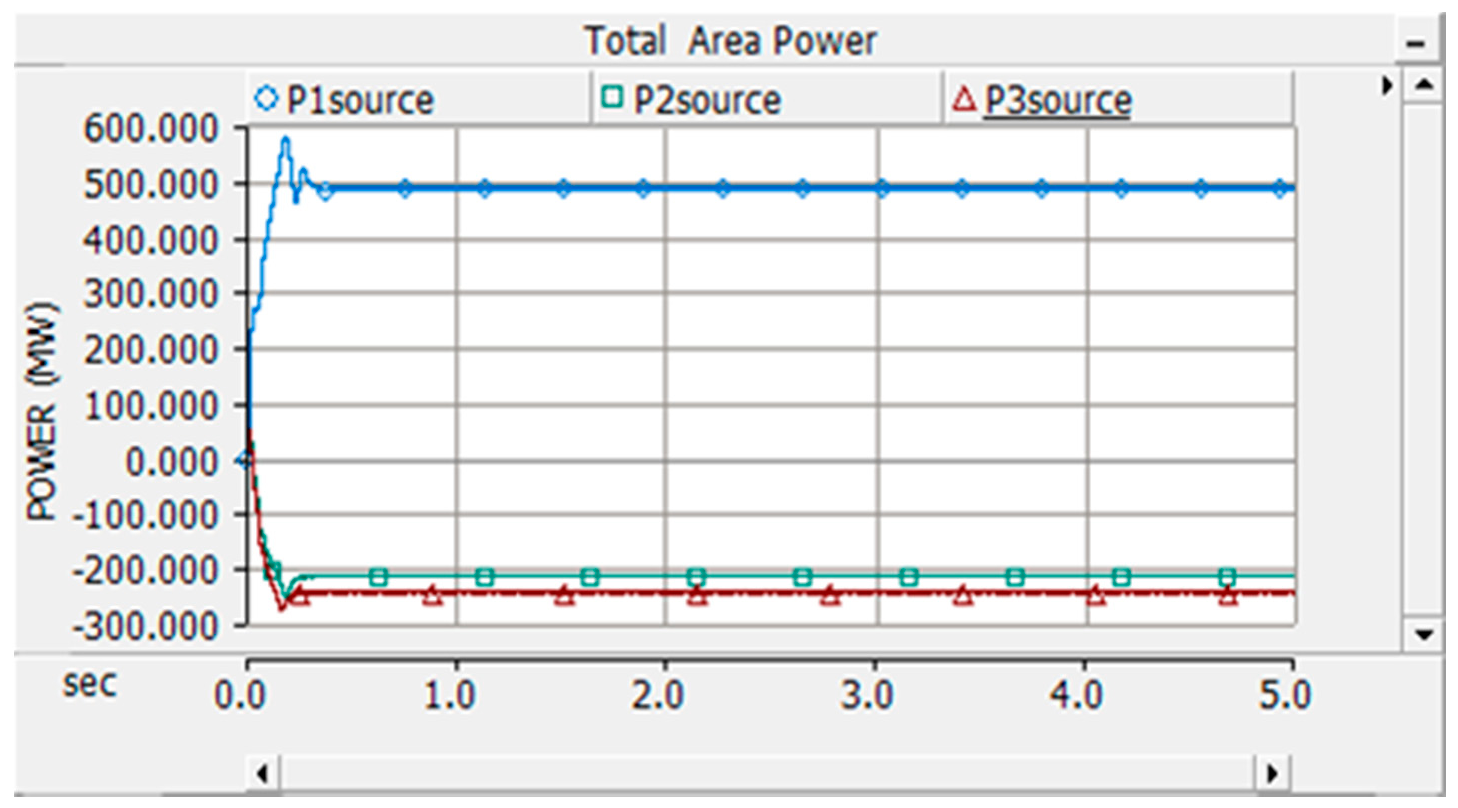
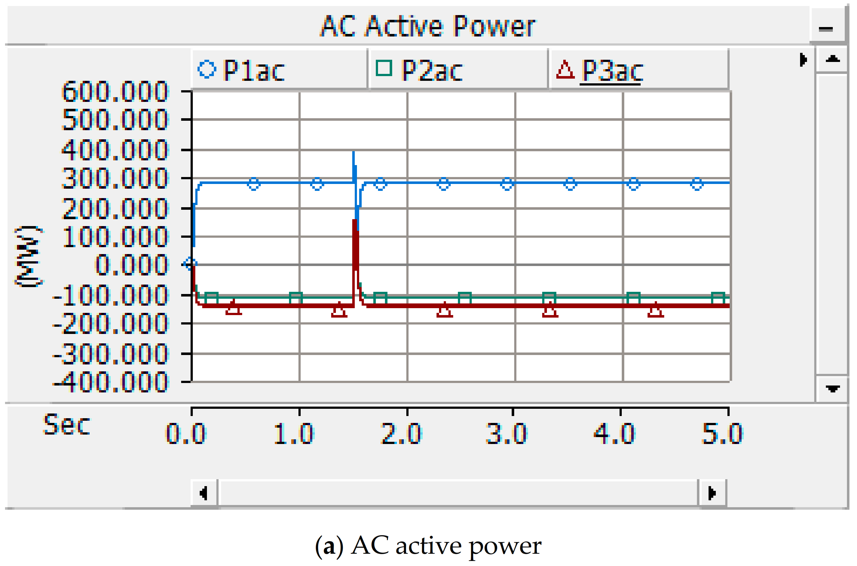
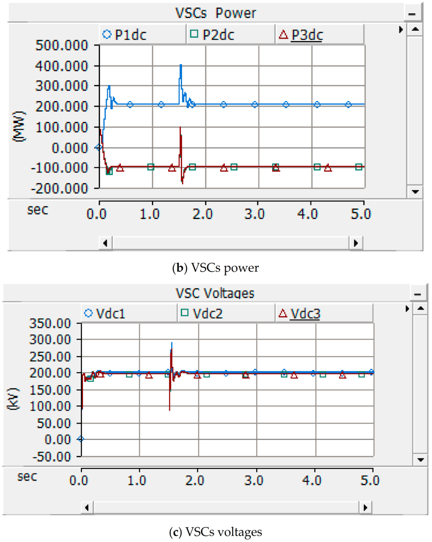
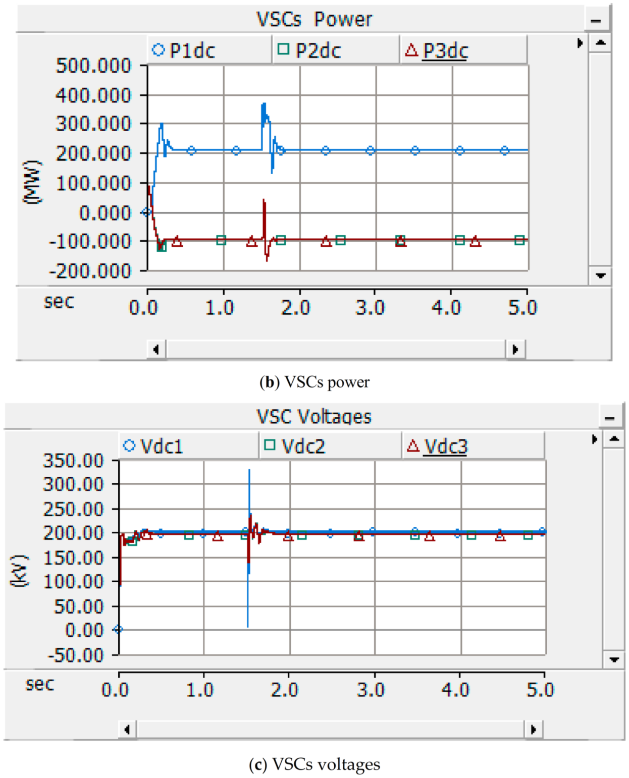
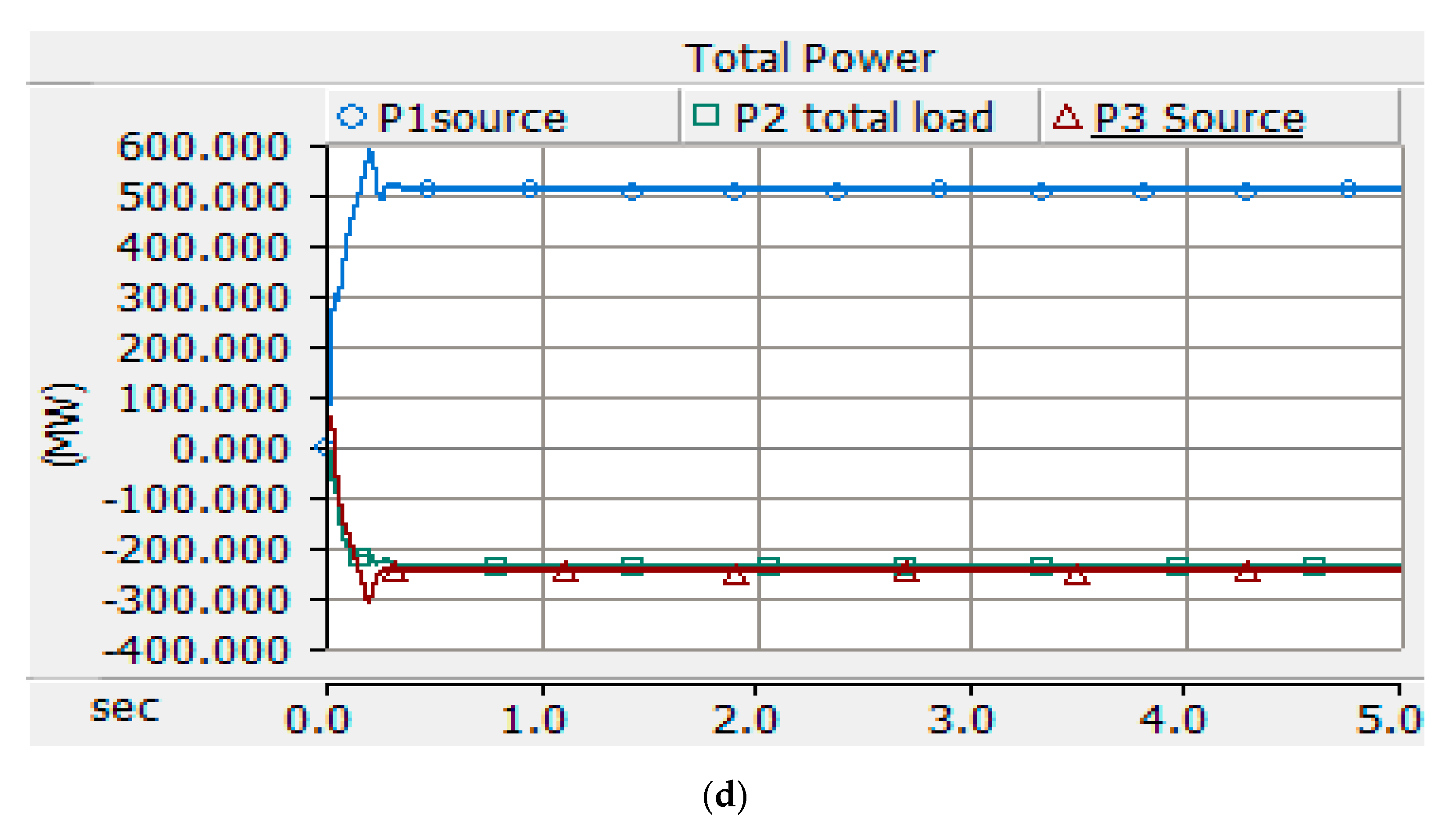
3.2. Case 1: All Three Areas Connected to the Source

Figure 1 was modeled in digital simulation software PSCAD/EMTDC and is shown in Figure 6. The DC voltage was controlled by VSC1, whereas VSC2 and VSC3 controlled active and reactive power flow. The system had three power system areas: area-1, area-2, and area-3; each area consisted of an AC source, zig-zag transformer, and VSC. The DC voltage was maintained by VSC1 using a PI controller and regulated by active current i_d and reference active current i_dref. DC was the reference input to the inner current controller.

Simulated results show that DC voltages of 200 kV are maintained constant at all three terminals of the proposed system and are shown in Figure 7. V_dc1, V_dc2, and V_dc3 represent the DC terminal voltage of VSC1, VSC2, VSC3, respectively.

Table 2. Active power flow for all three power system areas; (power are in MW).

Reference Power		Area-1 Active Power		Area-2 Active Power		Area-3 Active Power		Ptotal Active Power
Pref2	Pref3	P1ac	P1dc	P2ac	P2dc	P3ac	P3dc	P1source	P2source	P3source
−100	−100	278	204.7	−118.7	−98.8	−147.4	−98.81	482.8	−217.5	−246.21
−100	−50	278	152.9	−118.7	−98.8	−147.4	−48.81	430.9	−217.5	−196.21
−50	−100	278	152.7	−118.7	−48.7	−147.4	−98.78	430.7	−167.4	−246.18
−50	−50	278	101.4	−118.7	−48.7	−147.4	−48.76	379.4	−167.4	−196.16
100	100	−265.5	−196.2	123.6	101.4	153.8	101.4	−461.7	225.1	255.3

shows the recorded data of active power flow for all three power system areas with a power angle ($\delta$) of 30° between sending end source to receiving end source and different VSCs power reference settings.

When reference power for VSC2 and VSC3 is negative, power flows from area-1 to area-2 and area-3. When the polarities of VSC2 and VSC3 are changed, the direction of power flow is also reversed. If P_ref2 and P_ref3 of VSC2 and VSC3 are set at −100 MW, positive power flows from area-1 to area-2 and area-3. Power flowing in area-2 and area-3 is negative, which means power is flowing into the source.

When VSC3 reference power is changed to −50 MW, only DC power flowing through area-3 is changed, while the power flow in other areas is unaffected. The simulated results shown in Figure 8a,b are pure AC power and DC power, respectively, flowing simultaneously through the same lines for the system operating at the condition stated in row 1 of Table 2.

When P_ref2 and P_ref3 are set at −50 MW and −100 MW, total DC power flowing from area-1 is 152.7 MW, DC power flow in area-2 and area-3 is −48.7 and −98.7 MW. AC power flow is the same as in previous cases. When P_ref2 and P_ref3 are set at 100 MW, in addition to the change in power angle, power flow is reversed, which means power flow from area-2 and area-3 to area-1 and is shown in the last row of Table 2.

AC and DC power flow in area-1 is negative, while power flowing in area-2 and 3 is positive. Total power flow in area-1, -2, and -3 is given by P_1source, P_2source, and P_3source, which is the sum of AC and DC power flow in each area as shown in Figure 9.

For the case of area-1, when it acted as sending mode while area-2 and area-3 acted as receiving ends, the DC power references for VSC2 and VSC3 were set at −100 MW. However, the power angle between sending end and receiving end sources was set at 45°. The simulation results for the above case are shown in Figure 10a–c.

The simulation results indicate DC power transfer remains the same while AC power transfer increases according to power angle, and both the powers flow independently. The difference in the total power in sending and receiving end is due to system losses.

4. System under Fault

Suppose the system under study operated at a condition indicated in row 1 of Table 2. A three-phase to ground timed fault of duration 0.03 s occurred at 1.5 s at the middle of the transmission line between areas-1 and -2 (i.e., near the tapping point for area-3). Near sending end, the results obtained are depicted in Figure 11 and Figure 12. Moreover, Figure 11 and Figure 12 represent simulated results of AC power, DC power, and DC voltage under the above-mentioned fault conditions and when the system was stable.

5. Case 2: Two Areas Connected to the Source and One Area Connected to Load

In this case, a simultaneous AC–DC network with three terminal VSC was constructed in PSCAD/EMTDC software. Area-1 and area-3 were connected to AC sources of 420 kV and 500 kV, respectively, whereas area-2 was connected to passive loads.

Table 3. Active power flow at all areas, (power is given in MW).

Reference Power		Area-1 Active Power		Area-2 Active Power		Area-3 Active Power		Ptotal Active Power
Pref2	Pref3	P1ac	P1dc	P2ac	P2dc	P3ac	P3dc	P1source	P2souce	P3source
−100	−100	274.06	228.94	−113.5	−121.0	−148.2	−98.81	503.012	−234.55	−247

provides the active power flow for all the three areas with VSCs power settings P_ref2 and P_ref3 of each −100MW. Area-1 and area-3 were connected to the source, while the passive load of 115 MW +20 MVAR was connected with a zig-zag-delta transformer, and 120MW +10MVAR load was connected with VSC2 in area-2.

The AC and DC power measured on the AC side of VSCs and VSCs voltages are shown in Figure 13. When all the area was connected to the source, active power for AC and DC was independently controlled and flowed in either direction. AC power could be controlled by changing the power angle between the two ends, and DC power changed with changing the reference power of VSC. Hence, active AC power and active DC power were controlled in either direction.

6. Economic Aspect

Transmission line costs comprise investment and operating costs. Investments accrue costs for the right of way (ROW), transmission towers, insulators, conductors, and terminal equipment. Operational costs mainly include the cost of losses. For simplicity, if it is supposed that the insulator characteristics are similar for DC and AC transmission and lines designed with the same insulation level, then it can be affirmed that a DC line carries the same power with two conductors (with positive and negative polarities with respect to ground) than an AC line with three conductors of the same size when operating individually. With the proposed solution, it can be possible to transfer simultaneous AC–DC power of the same rating with three conductors, which results in cost savings in comparison with a new HVAC or HVDC transmission line alone. Owing to environmental, right of way (ROW), and economic concerns in recent years, the installation of new transmission lines is very uneconomical to fulfill the increased demand for electricity. Therefore, with the proposed scheme, the increase in demand for electricity can be fulfilled by increasing the use of existing transmission lines, in addition to independent control of AC and DC power flow.

7. Conclusions

Simultaneous AC–DC power transmission is an approach to enhance the power transfer capability of existing lines to meet fast-growing demand without adding a new transmission line. A three-area power system was designed to verify the feasibility of a multi-terminal, simultaneous AC–DC system. The proposed model had two main components: a delta-zig-zag connected transformer and VSC in each area of the power system. In this interconnected, three-terminal, simultaneous AC–DC power transmission, one converter controlled the DC voltage, whereas the other two controlled the power in both directions. The vector control method was used to control both the active and reactive power flow independently. Reference power for VSC, which operated in “P” control mode, was set at a particular power level to validate the possibility of three-terminal, simultaneous AC–DC power transmission. The feasibility of the proposed model was verified by PSCAD/EMTDC software. Results confirm the independent control of AC and DC power in both directions, which is the novelty of this proposed solution. With the use of simultaneous AC–DC in the proposed solution, it is possible that transmission lines can be loaded up to their thermal limits, more power can be transmitted, and load demand can be fulfilled without installing new transmission lines, leading to cost savings in comparison with a new HVAC or HVDC transmission line alone.

References

1. Lachs, W.R.; Sutanto, D. Different types of voltage instability. IEEE Trans. Power Syst. 1994, 9, 1126–1134. [Google Scholar] [CrossRef]
2. Rahman, H.; Khan, B.H. Power upgrading of transmission line by combining AC-DC transmission. IEEE Trans. Power Syst. 2007, 22, 459–466. [Google Scholar] [CrossRef]
3. Basler, M.J.; Schaefer, R.C. Understanding Power-System Stability. IEEE Trans. Ind. Appl. 2008, 44, 463–474. [Google Scholar] [CrossRef]
4. Noroozian, M.; Angquist, L.; Ghandhari, M.; Andersson, G. Improving power system dynamics by series-connected FACTS devices. IEEE Trans. Power Deliv. 1997, 12, 1635–1641. [Google Scholar] [CrossRef]
5. Tan, Y.L.; Wang, Y. Effects of FACTS controller line compensation on power system stability. IEEE Power Eng. Rev. 1998, 18, 55–56. [Google Scholar] [CrossRef]
6. Edris, A. FACTS technology development: An update. IEEE Power Eng. Rev. 2000, 20, 4–9. [Google Scholar] [CrossRef]
7. Flourentzou, N.; Agelidis, V.G.; Demetriades, G.D. VSC-based HVDC power transmission systems: An overview. IEEE Trans. Power Electron. 2009, 24, 592–602. [Google Scholar] [CrossRef]
8. Bikash, M.; Sahoo, K. Dynamic Stability Improvement of Power System with VSC-HVDC Transmission; Science Publishing Corporation: Amman, Jordan, 2014; Volume 7, pp. 500–503. [Google Scholar]
9. Thams, F.; Suul, J.A.; Arco, S.D.; Molinas, M.; Fuchs, F.W. Stability of DC voltage droop controllers in VSC HVDC systems. IEEE Eindh. PowerTech. 2015, 1–7. [Google Scholar]
10. Cole, S.; Beerten, J.; Belmans, R. Generalized dynamic VSC MTDC model for power system stability studies. IEEE Trans. Power Syst. 2010, 25, 1655–1662. [Google Scholar] [CrossRef] [Green Version]
11. Beerten, J.; Cole, S.; Belmans, R. Generalized steady-state VSC MTDC model for sequential AC/DC power flow algorithms. IEEE Trans. Power Syst. 2012, 27, 821–829. [Google Scholar] [CrossRef] [Green Version]
12. Liang, J.; Jing, T. Operation and control of multiterminal HVDC transmission for offshore wind farms. IEEE Trans. Power Deliv. 2011, 26, 2596–2604. [Google Scholar] [CrossRef]
13. Zhang, L.; Zou, Y.; Yu, J.; Qin, J.; Vittal, V.; Karady, G.G.; Shi, D.; Wang, Z. Modeling, control, and protection of modular multilevel converter-based multi-terminal HVDC systems: A review. CSEE J. Power Energy Syst. 2017, 3, 340–352. [Google Scholar] [CrossRef]
14. Rahman, H.; Khan, B.H. Possibility of power tapping from simultaneous AC-DC power transmission lines. IEEE Trans. Power Deliv. 2008, 23, 1464–1471. [Google Scholar] [CrossRef]
15. Peterson, H.A.; Reitan, D.K.; Phadke, A.G. Parallel Operation of AC and DC Power Transmission. IEEE Trans. Power Appar. Syst. 1965, 84, 15–19. [Google Scholar] [CrossRef]
16. Pedra, J.; Sainz, L.; Monjo, L. Three-Port Small Signal Admittance-Based Model of VSCs for Studies of Multi-terminal HVDC Hybrid AC/DC Transmission Grids. IEEE Trans. Power Syst. 2020, 36, 732–743. [Google Scholar] [CrossRef]
17. Wang, P.; Goel, L.; Liu, X.; Choo, F.H. Harmonizing AC and DC: A Hybrid AC/DC Future Grid Solution. IEEE Power Energy Mag. 2013, 11, 76–83. [Google Scholar] [CrossRef]
18. Carroll, D.P. Coordinated active and reactive power modulation of multiterminal HVDC systems. IEEE Trans. Power Appar. Syst. 1984, 6, 1480–1485. [Google Scholar]
19. Wang, H.; Tang, G.; He, Z.; Yang, J. Efficient Grounding for Modular Multilevel HVDC Converters (MMC) on the AC Side. IEEE Trans. Power Deliv. 2014, 29, 1262–1272. [Google Scholar] [CrossRef]
20. Abdelwahed, M.A.; El-Saadany, E.F. Power Sharing Control Strategy of Multiterminal VSC-HVDC Transmission Systems Utilizing Adaptive Voltage Droop. IEEE Trans. Sustain. Energy 2017, 8, 605–615. [Google Scholar] [CrossRef]
21. Gonzalez-Longatt, F.; Roldan, J. Effects of DC Voltage control strategy on voltage response on multi-terminal HVDC following loss of a converter station. In Proceedings of the IEEE Power and Energy Society General Meeting, Vancouver, BC, Canada, 21–25 July 2013. [Google Scholar]
22. Zhang, L.; Harnefors, L.; Nee, H. Modeling and Control of VSC-HVDC Links Connected to Island Systems. IEEE Trans. Power Syst. 2011, 26, 783–793. [Google Scholar] [CrossRef]
23. Castro, L.M.; Acha, E. A Unified Modeling Approach of Multi-Terminal VSC-HVDC Links for Dynamic Simulations of Large-Scale Power Systems. IEEE Trans. Power Syst. 2016, 31, 5051–5060. [Google Scholar] [CrossRef]
24. Li, Z.; He, Y.; Li, Y.; Gu, W.; Tang, Y.; Zhang, X. Hybrid Control Strategy for AC Voltage Stabilization in Bipolar VSC-MTDC. IEEE Trans. Power Syst. 2019, 34, 129–139. [Google Scholar] [CrossRef]
25. Yazdani, A.; Iravani, R. Voltage-Sourced Converters in Power Systems: Modeling, Control, and Applications; John Wiley & Sons: Hoboken, NJ, USA, 2010. [Google Scholar]
26. Rahman, H.; Khan, B.H. Stability improvement of power system by simultaneous ac-dc power transmission. Electr. Power Syst. Res. 2007, 78, 756–764. [Google Scholar] [CrossRef]
Figure 1. (a) Zig-zag connection of transformer; (b) block diagram of three-terminal, simultaneous AC–DC power transmission.
Electronics 11 00108 g001aElectronics 11 00108 g001b
Figure 2. (a) Simplified structure of VSC station controllers; (b) schematic diagram of VSC.
Electronics 11 00108 g002aElectronics 11 00108 g002b
Figure 3. Equivalent circuit of d and q axes of VSC.
Electronics 11 00108 g003
Figure 4. Inner current controller diagram.
Electronics 11 00108 g004
Figure 5. Control for (a) active power, (b) reactive power, (c) DC voltage control, and (d) DC voltage control.
Electronics 11 00108 g005
Figure 6. Simulated model in PSCAD/EMTDC for case 1.
Electronics 11 00108 g006
Figure 7. DC voltage at (a) VSC1, (b) VSC2, and (c) VSC3 terminals, respectively.
Electronics 11 00108 g007
Figure 8. (a) Pure AC power in area-1, area-2, and area-3; (b) active power flow measured on AC side of VSC1, VSC2, and VSC3.
Electronics 11 00108 g008
Figure 9. Total active power in area-1, area-2, and area-3.
Electronics 11 00108 g009
Figure 10. Power flow at power angle of 45°: (a) AC power flow in area-1, area-2, and area-3 as P1ac, P2ac, and P3ac, respectively; (b) DC power flow in area-1, area-2, and area-3 as P1dc, P2dc, and P2dc, respectively; (c) total power flow in area-1, area-2, and area-3 as P1source, P2source, and P3source, respectively.
Electronics 11 00108 g010aElectronics 11 00108 g010b
Figure 11. Three-phase to ground fault at the middle of the transmission line for 0.03 s duration.
Electronics 11 00108 g011aElectronics 11 00108 g011b
Figure 12. Three-phase to ground fault at sending end of transmission line for 0.03 s duration.
Electronics 11 00108 g012aElectronics 11 00108 g012b
Figure 13. Simulated results for case 2. (a) DC terminal voltages of VSC1, VSC2, and VSC3. (b) Power measured on AC side of VSC1, VSC2, and VSC3. (c) Power measured on DC side of VSC1, VSC2, and VSC3. (d) Total power in area-1, area-2, and area-3.
Electronics 11 00108 g013aElectronics 11 00108 g013b