Abstract
Recent research has focused on sustainable development and renewable energy resources, thus motivating nonconventional cutting-edge technology development. Multilevel inverters are cost-efficient devices with IGBT switches that can be used in ac power applications with reduced harmonics. They are widely used in the power electronics industry. However, under extreme stress, the IGBT switches can experience a fault, which can lead to undesirable operation. There is a need for a reliable system for detecting switch faults. This paper proposes a signal processing method to detect open-circuit problems in IGBT switches. Relative wavelet energy has been used as a feature for a machine learning algorithm to diagnose and classify the faulted switches. The switching sequence can be altered to restore a healthy output voltage. Inverter faults have been diagnosed by using support vector machine (SVM) and decision tree (DT), and an ensemble model based on decision tree (DT) and XG boost algorithm was developed, which yielded 92%, 88%, and 94.12% accuracy, respectively.
1. Introduction
A surge in the development of renewable energy resources has made it crucial to supply high-quality electrical energy to various electrical loads. Renewable power is increasingly being converted into grid-compatible and standalone forms by power converters. The DC–AC converters, also called inverters, are used to convert the DC power produces by the solar PV generation system into AC power that is fed to the grid or used for industrial applications. In comparison to conventional two-level inverters, multilevel inverters generate lower harmonic voltage/current, since they are characterized by a multilevel quasi-sinusoidal waveform. Various multilevel inverter topologies have been proposed in the literature, such as the PUC5 topology [1,2,3,4,5,6,7,8,9,10,11,12,13], which was introduced to provide good quality power and reduce the number of components compared to its predecessors. Insulated gate bipolar transistors (IGBT) are typically used as power switches in multilevel inverters due to their high voltage and current ratings.
Nevertheless, unexpectedly high current due to a fault in line or due to aging effect results in IGBT failure under excessive thermal and electrical stress. IGBT faults include short circuit faults, with the latter being more common. If a short circuit fault occurs, it can easily be identified. If necessary, the circuit can be isolated. It has been discussed [3] how to detect short circuits and open circuits. When an open-circuit fault occurs, it does not have any noticeable effect immediately after the event. As time passes, however, open-circuit faults can cause temporary paralysis of the system, and faults in IGBT switches can result in increased THD in the output of a multilevel inverter. Thus, a robust fault detection and localization method are essential to identify the fault as soon as possible.
The literature has demonstrated a variety of techniques for fault detection and isolation. According to Reference [1], the adaptive electrical period partition (AEPP) algorithm picks single electrical periods from real-time three-phase current signals to identify faults. The signal is analyzed using maximal overlap DWT and Park’s vector modulus, and then, random forest is used to classify faults. An alternative strategy that uses discrete wavelet transform for capacitor current and switch current data and uses machine learning techniques such as artificial neural networks (ANN), k-nearest neighbor(KNN), support vector machines(SVM), and decision tree (DT) has been proposed in Reference [2]. An ANN performs diagnosis accurately but requires vast amounts of data for learning; as a result, the accuracy of the network relies on the amount of data. A three-phase current analysis for diagnosing the open-circuit faults for single and multiple switches is presented [3]. The method is based on normalized mean current park’s vector modulus, and an angle that involves only three-phase output current was proposed in Reference [4]. A cascaded h-bridge (CHB) multilevel inverter can be diagnosed by monitoring each cell’s output voltage and current direction. The technique has been implemented using level-shifted pulse width modulation (LS-PWM) in order to achieve an acceptable total harmonic distortion (THD), as described in Reference [5]. The use of multilayer perceptron’s for classification and localization of the fault type is discussed in Reference [6]. A hybrid intelligent algorithm such as discrete wavelet transform (DWT) and neural networks (NN) is discussed in Reference [7]. Various other topologies for detecting a fault in multilevel inverters were proposed in Reference [8], such as three-legged topologies, four-legged topologies, FC legs, and inductor-based fourth-leg topologies. Methods based on the measurement of the output phase voltage or phase current were presented in Reference [9]. Several other methods for detecting an open-circuit fault in a multilevel inverter were discussed in Reference [10]. An online diagnostic method for open-circuit switch faults T-type multilevel inverters based on SiC-MOSFETs was discussed in Reference [14]. The proposed fault diagnosis and fault-tolerant control scheme for flying capacitor multilevel inverters was presented in Reference [15]. A generalized model for switch fault diagnosis for cascaded H-bridge multilevel inverters using mean voltage prediction was proposed in Reference [16]. Neutral point-clamped inverter fault detection is based on the failure mode algorithm [17]. The fault diagnosis of a cascaded H-bridge multilevel inverter system fault diagnosis using a PCA and multiclass relevance vector machine was in Reference [18]. A fault detection method for three-level inverters was presented in Reference [19] based on DC-bus electromagnetic signatures. A short-circuit fault diagnosis method for three-phase inverters was proposed in Reference [20]. Fault tolerance techniques for three-phase voltage source inverters was described in Reference [21]. Topologies for single-phase and three-phase applications were discussed in Reference [22]. A multilevel inverter with minimized components featuring self-balancing and boosting capabilities for PV applications was presented in Reference [23]. Linear modulation range extension to the full base speed using a single DC link multilevel inverter with capacitor-fed H-bridges for IM drives was in Reference [24]. Comparison of impedance source networks for two- and multilevel Buck-Boost inverter applications were in Reference [25]. A fault tolerance system mainly has three main components: redundancy, fault detection, and an isolation system and reconfiguration system. A good detection technique can increase the system’s reliability and robustness. More recently, a novel packed U-cell (PUC-5) topology was proposed with significantly less switch utilization and five output voltage levels. However, no fault was conducted on the PUC-5 topology.
The primary goal of this work is to detect open-circuit faults in IGBT switches in packed unit cell (PUC) 5 multilevel inverters as early as possible by using classical machine learning models. The focus of this study is not to determine which of the switches is more susceptible to a fault but, rather, to identify the fault in any switch that occurs. Most of the algorithms documented are state-of-the-art and discussed above used time domain sampled values as machine learning features. It is necessary to develop a robust feature in the time–frequency domain that can be discriminated at the gateway of ML models to detect open-circuit faults. This paper presents a novel method for generating reliable time–frequency domain features by applying discrete wavelet transform (DWT) [14] and analyzing the power spectral density (PSD). At the same time, the second contribution deals with developing a more accurate machine learning model in this context. We propose two conventional and ensemble machine learning models for six mutually exclusive switch fault detection types in PUC 5 multilevel inverter topology by utilizing distinguishable sub-hand relative wavelet energies as features.
2. Multilevel Inverter
2.1. Packed U-Cell 5 (PUC-5) Topology
The multilevel inverter topology shown in Figure 1 is PUC-5 topology. A comparative study of the various topologies was done in Reference [11], with PUC-5 emerging as a very tough competitor. The packed unit cell topology was first introduced in 2010 as a 7-level inverter to provide good quality power conversion and reduce the number of components. In 2015, its 5-level version, PUC-5 topology, derived from 7-level topology, was proposed, which generated a 5-level voltage waveform. The capacitor voltage balancing process was simple. It does not require any external controllers, making a 5-level converter a competitor in power electronics inverters [12].
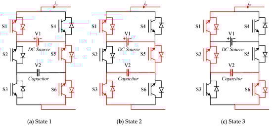
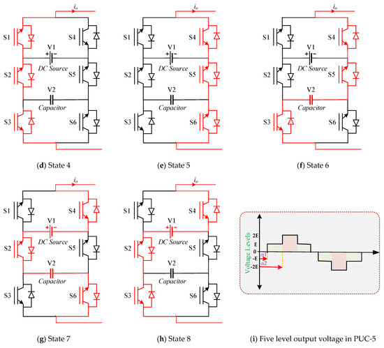
Figure 1.
(a–h) Various PUC-5 inverter switching states and (i) five-level output in PUC-5.
The 5-level PUC inverter topology utilizes a single DC source and a capacitor. It produces voltage levels. The key advantage of the 5-level topology is the redundant switching states and single DC source, which are necessary for effective voltage balancing without using an external controller. The switching states and their effects on capacitor voltages are shown in Table 1, where Vdc = 2E and Vc = E. From the table, it can be inferred that the characteristic feature of PUC-5 configuration is the redundant states, which help balance the auxiliary capacitor voltage by providing different paths with the same voltage level at the output [13]. States (2, 3) and (6, 7) are redundant states. The voltage outputs of the PUC-5 inverter in normal conditions and in the fault in each IGBT switch are shown in Figure 2.

Table 1.
Switching Table.
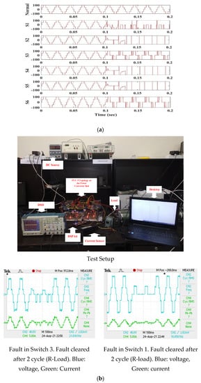
Figure 2.
(a) Simulated output voltage waveforms under various faults. (b) Experimental output voltage waveforms under two different switch faults.
Due to its configuration structure, the PUC inverter is called a packed U-cell inverter.
The switching function of the PUC inverter is defined as
The inverter output voltage can be written as
The voltage across the point can be calculated according to the switching function:
where V1 and V2 are the main DC-link voltage and capacitor voltage, respectively.
Since one of the switches in pairs of T1 and T4, T2 and T5, and T3 and T6 is turned ON, the current in the switches can be expressed with respect to the current in the load as
By applying KCL at node c, we get the following:
and
For the current (in the load) and the voltage, the Kirchhoff voltage law is expressed as follows:
where Rf and Lf are the filter resistance and inductance, respectively.
Assuming the state variables as x1 = i1 and x2 = V2 and using duty cycles (d1, d2, and d3) of switches (T1, T2, and T3) as the input matrix, the state–space average model of the packed U-cell inverter may be obtained as follows:
The above state–space model can design the controller to regulate the capacitor voltage to a particular value to get the desired multilevel output voltage.
2.2. Operation under Different Fault Conditions
The PUC-5 inverter was operated under normal and various fault conditions. The simulation voltage waveforms for faults in different switches S1–S8 are shown in Figure 2. PUC-5 was also assembled on a power converter testbed, and voltage waveforms for the faults in switches S1–S8 were observed.
3. Fault Diagnosis Method
Figure 3 shows the flowchart of the open-circuit fault detection system. When the multilevel inverter runs, the system monitors the voltage output waveform and extracts features from the waveform; the features are input into the classifier, which classifies the faults in different switches and returns the faulty switch as the output.
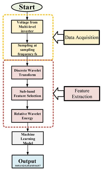
Figure 3.
Flowchart of the diagnosis system.
The Simpower toolbox in Simulink was used to simulate data of fault with modulation index (ma) values varying from 0.1 to 1.0. The voltage output for the switch faults is shown in Figure 2. One can see that the faults for the outputs can be perceptually separated. However, the computation unit cannot directly distinguish the faults, as the signals are nonstationary. Therefore, a signal transformation technique is required. An appropriate selection of feature extraction is necessary to provide the classifier with adequate significant details in the pattern set so that the highest accuracy is obtained. One technique that can be considered is discrete wavelet transform, a comparative study of feature extraction for fault detection using various techniques that was presented in Reference [26].
3.1. Feature Extraction—Discrete Wavelet Transform
A wavelet is a square-integrable function with constant energy, which is very effective in sub-band filtering techniques. The DWT employs extensive time windows for low frequencies and small time windows for high frequencies, which enables both high-resolution and low-resolution feature extraction. DWT uses subsequent high-pass filters, low-pass filters, and downsampling by a factor of two for the decomposition of nonstationary signals, as shown in Figure 4. The high-pass filter g[n] is the discrete mother wavelet, and the low-pass filter is its scaling function. Figure 5 is the output of the discrete mother wavelet, and its scaling functions have appertained as an approximation. The detailed coefficients are shown by A1 and D1, respectively.
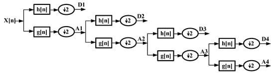
Figure 4.
DWT decomposition.
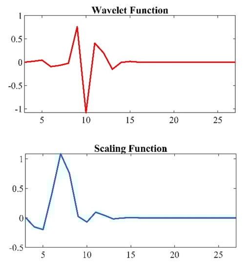
Figure 5.
Sym7 mother wavelet and scaling function.
Wavelet transform uses multiple low-pass and high-pass filters followed by downsampling by a factor of two; to decompose a nonstationary signal, the low-pass filter or the scaling function is given by , and the high-pass filter or wavelet function is given by ; together, the two functions on all the decomposition levels cover the complete frequency spectrum, the filter functions are convolved with the input signal, and the output of the convolution is downsampled by two to remove the redundant samples and to make sure that, even after reconstruction of the signal, the number of samples in the reconstructed signal is equal to the input signal. The scaling function is dependent on the low-pass filter, and the wavelet function depends upon the high- pass filter and are denoted as follows [27]:
The maximum levels of decomposition are specified based on the frequency components of interest in the given signal; the coefficients of DWT are referred to as the dot product of the signal and wavelet basis functions, and the approximation coefficients and detailed coefficients Ai and Di are denoted as
where k = 0,1,2,.., 2j–1, and N is the length of the discrete signal.
The wavelet energy at each decomposition level i = 1,…, L is computed as
where i = 1,2,3,…,L.
where i = L.
The total and relative sub-band energies are calculated as follows:
The normalized energy values represent the relative wavelet energy
where Ej = or
Table 2 shows the approximation and detail coefficients and their frequency sub-bands.
Table 2.
The Frequency Band for the Wavelet Coefficients.
The extraction of relevant information from a given signal is crucial, as it directly affects the classifier performance. To extract the relevant features, we sorted out the sub-bands for wavelet energy calculation by plotting the power spectral density curves shown in Figure 6 for all the cases at a particular modulation index and selected the bands in which all the curves were distinguishable. Figure 7 shows the scatterplot or the relative wavelet energies of the A4 and D1 coefficients at different modulation indices. We employed relative wavelet energy to compare a distorted signal with a normal one, and the relative wavelet energy was calculated using Equation (19).
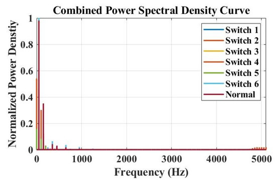
Figure 6.
Power spectral densities of open-circuit faults.
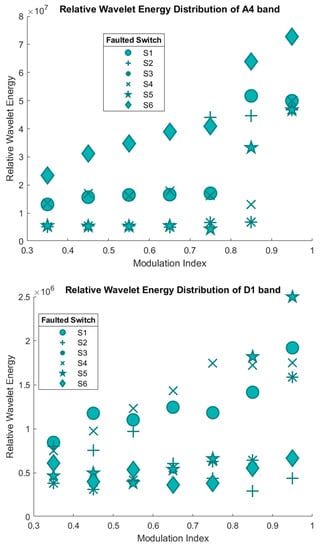
Figure 7.
Wavelet energies of the A4 and D1 bands.
3.2. Classification Methods
A classifier uses an algorithm that learns from various nondependent variable values called features as the input and predicts the corresponding class to which the independent variable belongs. In signal processing, features can be energy, entropy, transform coefficients, etc. A classifier that is updated during the classifier training from the training data. The learned classifier model is an association between the features and the classes. For example, for a given classifier for a given feature x, there is a corresponding class y; the classifier algorithm is a function that predicts that class as y = f(x). After training, the classifier can predict instances of classes that were not used in the training data. Thus, the performance of a classifier is tested on a different set of instances.
3.3. Support Vector Machines
To demonstrate the effectiveness of the proposed feature extraction scheme in classification, the SVM classifier was used. SVM is a supervised machine learning algorithm derived from statistical learning theory [28] applied in both classification and regression tasks; SVM maps the original pattern space into the high-dimensional space by nonlinear mapping functions, such that an optimal separating hyperplane can be constructed in the feature space. Thus, a nonlinear problem in low-dimensional space corresponds to a linear problem in high-dimensional space [29]. Figure 8 shows the SVM diagram. It shows how the SVM separates the data into extreme points, which can be separated using a hyperplane, where the points lying on the line are the support vectors.
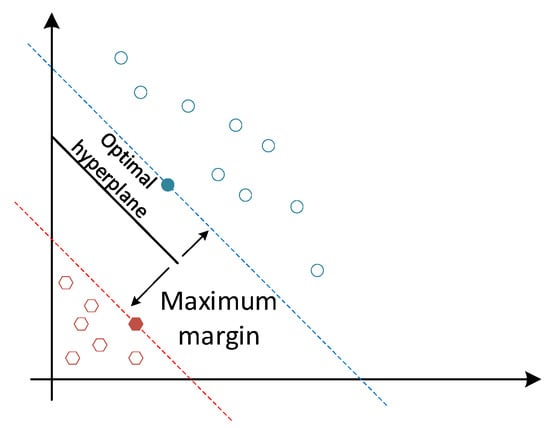
Figure 8.
Hyperplane Visualization of SVM classifier.
3.4. Decision Trees
A decision Tree is a supervised machine learning algorithm that uses a training set of mutually exclusive classes that are known, and the algorithm determines the class of an input using the attributes of the input object. The DT method represents the decision to be made graphically and employs a top-to-bottom strategy to obtain all possible outcomes and searches for the optimum output. Each decision node in the tree uses a feature to classify the input x into y classes. The decision tree diagram is shown in Figure 9.
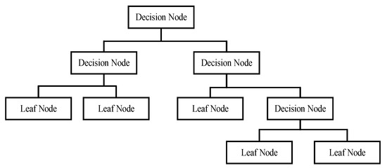
Figure 9.
Decision Tree Diagram.
3.5. XG Boost
XG Boost algorithm or Extreme boost is a gradient boosting algorithm based on the Newton Raphson method for scalable end-to-end tree boosting, involving the bagging method for combining decisions from parallel classification using parallelization for sequential tree building and pruning as a mechanism for stopping.
4. Results and Discussion
The classifiers were trained on the extracted features, relative wavelet energies of sub-bands A4 and D1, by splitting the dataset into training (70%) and testing (30%) data. Seven classes were available: a fault occurred in one out of six, followed by normal operations. There were three classifiers used: SVM, DT, and ensemble models based on classical machine learning. Accuracy, precision, recall, and F1-score were used to evaluate the performances. In order to understand the reliability of introducing these parameters for performance comparison, we should be familiar with some machine learning terms. Therefore, the four basic terms are defined as follows:
- True Positive (TP): outcome where the model correctly predicts the positive class.
- True Negative (TN): outcome where the model correctly predicts the negative class.
- False Positive (FP): outcome where the model wrongly predicts the positive class.
- False Negative (FN): outcome where the model wrongly predicts the negative class.
The first stage with SVM started with default hyperparameters such as C = 1 and kernel = RBF, then extended our experiment with a grid search for three hyperparameters, including regularization parameter (C), kernel type, and kernel coefficient values, taking values out, respectively (0.1, 1, 10, 100, and 1000), (Radial Basis Function (RBF), Linear), and (0.1, 1, 10, 100, and 1000), respectively, for a brute force analysis. The second stage was to implement a classifier based on a decision tree and to train it using the default hyperparameters of splitting criteria = gini and number of splitting samples = 2. For improving the training performance considerably, we employed ensemble modeling of DT with the Extreme Gradient (XG) boosting algorithm by setting up the following parameters: boosting function, step size shrinkage, maximum depth, minimum child weight, maximum delta step, subsample ratio, sampling method, L1 regularization value, and L2 regularization value, so that they were “GBtree”, 0.3, 0, 6, 1, 0, 1, “uniform”, 1, and 0, respectively. For the A4 and D1 coefficients, the classification process was implemented by implementing the extracted features. Table 3 shows the classification report for the classifiers with the metrics accuracy, precision, recall, and F1-scores with the classifiers maintaining accuracy of 92% for SVM, 88% accuracy for the decision tree, and 94.12% accuracy for the boosted decision tree for the extracted features, whereas the remaining three metrics yielded approximately the same numerical values for these three classifiers.
Table 3.
Performance metrics for Machine Learning classifiers.
5. Conclusions
This paper presented a robust approach to fault diagnosis in multilevel inverters using sub-band relative wavelet energies as features with machine learning algorithms for classification. Each fault case voltage output for each fault case, in a window of 0.2 s, was sampled at a sampling frequency of 10 kHz, and the sampled output was divided into sub-bands using the DWT approach with Symlets (Sym7) wavelets, and the sub-band energies were calculated for the frequency range of interest based on a power spectral density comparison of the sampled output. According to the results, the most exploitable bands were A4 and D1, corresponding to 0–625 Hz and 2500–5000 Hz, respectively. The support vector machines, decision tree, and gradient boosted decision tree algorithms were used to classify the test dataset, with 92%, 88%, and 94.12% accuracy, respectively. These methods can be used for detecting faults in various other multilevel inverter topologies.
Author Contributions
Conceptualization, A.S., F.A.K., F.S. and V.B.; methodology, F.A.K.; software, A.S. and F.S.; validation, A.S., M.M.S., S.A., and M.I.; formal analysis, A.S. and F.A.K.; investigation, M.F.A., F.A.K. and V.B.; resources, M.M.S., S.K., M.I. and S.A.; data curation, F.A.K. and V.B.; writing—original draft preparation, A.S., F.A.K. and V.B.; writing—review and editing, A.S., F.A.K., F.S., M.I. and V.B.; visualization, A.S., M.M.S. and S.K.; supervision, M.F.A., A.S. and M.I.; project administration, A.S., M.I., M.M.S. and S.A; funding acquisition, M.F.A., S.A., M.I., S.K. and M.M.S. All authors have read and agreed to the published version of the manuscript.
Funding
The researchers would like to thank the Deanship of Scientific Research, Qassim University, Saudi Arabia and Department of Electrical Engineering, College of Engineering and Information Technology, Unaizah Colleges, Unaizah, Saudi Arabia for funding the publication of this project.
Data Availability Statement
Not Applicable.
Conflicts of Interest
The authors declare no conflict of interest.
Notations
| Vdc | Source Voltage |
| Vc | Voltage across Capacitor |
| Wavelet Function | |
| Scaling Function | |
| Approximation Coefficient for ith Sub-Band | |
| Detail Coefficient for ith Sub-Band | |
| Energy of Detail Coefficient | |
| Energy of Approximation Coefficient | |
| Total Energy of A and D coefficients | |
| Relative Energy of Each sub band |
References
- Liu, S.; Qian, X.; Wan, H.; Ye, Z.; Wu, S.; Ren, X. NPC Three-Level Inverter Open-Circuit Fault Diagnosis Based on Adaptive Electrical Period Partition and Random Forest. J. Sensors 2020, 2020, 9206579. [Google Scholar] [CrossRef] [Green Version]
- Achintya, P.; Sahu, L.K. Open Circuit Switch Fault Detection in Multilevel Inverter Topology using Machine Learning Techniques. In Proceedings of the IEEE 9th Power India International Conference (PIICON), Sonepat, India, 28 February–1 March 2020; pp. 1–6. [Google Scholar]
- Cheng, S.; Zhao, J.; Chen, C.; Li, K.; Wu, X.; Yu, T.; Yu, Y. An open-circuit fault-diagnosis method for inverters based on phase current. Transp. Saf. Environ. 2020, 2, 148–160. [Google Scholar] [CrossRef]
- Sital-Dahone, M.; Saha, A.; Sozer, Y.; Mpanda, A. Multiple device open circuit fault diagnosis for neutral-point-clamped inverters. In Proceedings of the 2017 IEEE Applied Power Electronics Conference and Exposition (APEC), Tampa, FL, USA, 26–30 March 2017; pp. 2605–2609. [Google Scholar] [CrossRef]
- Mhiesan, H.; Umuhozs, J.; Mordi, K.; McCann, R.; Balda, J.C.; Farnell, C.; Mantooth, A. A Method for Open-Circuit Faults Detecting, Identifying, and Isolating in Cascaded H-Bridge Multilevel Inverters. In Proceedings of the 9th IEEE International Symposium on Power Electronics for Distributed Generation Systems (PEDG), Charlotte, NC, USA, 25–28 June 2018. [Google Scholar]
- Khomfoi, S.; Tolbert, L. Fault Diagnostic System for a Multilevel Inverter Using a Neural Network. IEEE Trans. Power Electron. 2007, 22, 1062–1069. [Google Scholar] [CrossRef]
- Xu, J.; Song, B.; Zhang, J.; Xu, L. A new approach to fault diagnosis of multilevel inverter. In Proceedings of the 2018 Chinese Control And Decision Conference (CCDC), Shenyang, China, 9–11 June 2018; pp. 1054–1058. [Google Scholar] [CrossRef]
- Lezana, P.; Pou, J.; Meynard, T.; Rodriguez, J.; Ceballos, S.; Richardeau, F. Survey on Fault Operation on Multilevel Inverters. IEEE Trans. Ind. Electron. 2009, 57, 2207–2218. [Google Scholar] [CrossRef] [Green Version]
- Da Silva, E.; Lima, W.; de Oliveira, A.; Jacobina, C.; Razik, H. Detection and compensation of switch faults in a three level inverter. In Proceedings of the 37th IEEE Power Electronics Specialists Conference, Jeju, Korea, 18–22 June 2006. [Google Scholar] [CrossRef]
- Lu, B.; Member, S.; Sharma, S.K. A Literature Review of IGBT Fault Diagnostic and Protection Methods for Power Inverters. IEEE Trans. Ind. Appl. 2009, 45, 1770–1777. [Google Scholar]
- Ounejjar, Y.; Al-Haddad, K.; Grégoire, L.-A. Packed U Cells Multilevel Converter Topology: Theoretical Study and Experimental Validation. IEEE Trans. Ind. Electron. 2010, 58, 1294–1306. [Google Scholar] [CrossRef]
- Pakdel, M.; Jalilzadeh, S. A New Family of Multilevel Grid Connected Inverters Based on Packed U Cell Topology. Sci. Rep. 2017, 7, 12396. [Google Scholar] [CrossRef] [Green Version]
- Vahedi, H.; Sharifzadeh, M.; Al-Haddad, K. Topology and Control Analysis of Single-DC-Source Five-Level Packed U-Cell Inverter (PUC5). In Proceedings of the IECON 2017–43rd Annual Conference of the IEEE Industrial Electronics Society, Beijing, China, 29 October–1 November 2017; pp. 1–6. [Google Scholar]
- He, J.; Demerdash, N.A.O.; Weise, N.; Katebi, R. A Fast On-Line Diagnostic Method for Open-Circuit Switch Faults in SiC-MOSFET-Based T-Type Multilevel Inverters. IEEE Trans. Ind. Appl. 2017, 53, 2948–2958. [Google Scholar] [CrossRef]
- Amini, J.; Moallem, M. A Fault-Diagnosis and Fault-Tolerant Control Scheme for Flying Capacitor Multilevel Inverters. IEEE Trans. Ind. Electron. 2016, 64, 1818–1826. [Google Scholar] [CrossRef]
- Anand, A.; Vinayak, B.A.; Raj, N.; Jagadanand, G.; George, S. A generalized switch fault diagnosis for cascaded h-bridge multilevel inverters using mean voltage prediction. IEEE Trans. Ind. Appl. 2019, 56, 1563–1574. [Google Scholar] [CrossRef]
- Ahmadi, S.; Poure, P.; Saadate, S.; Khaburi, D.A. A Real-Time Fault Diagnosis for Neutral-Point-Clamped Inverters Based on Failure-Mode Algorithm. IEEE Trans. Ind. Informatics 2021, 17, 1100–1110. [Google Scholar] [CrossRef]
- Wang, T.; Xu, H.; Han, J.; Elbouchikhi, E.; Benbouzid, M.E.H. Cascaded H-Bridge Multilevel Inverter System Fault Diagnosis Using a PCA and Multiclass Relevance Vector Machine Approach. IEEE Trans. Power Electron. 2015, 30, 7006–7018. [Google Scholar] [CrossRef]
- Abari, I.; Lahouar, A.; Hamouda, M.; Slama, J.B.H.; Al-Haddad, K. Fault Detection Methods for Three-Level NPC Inverter Based on DC-Bus Electromagnetic Signatures. IEEE Trans. Ind. Electron. 2017, 65, 5224–5236. [Google Scholar] [CrossRef]
- Alavi, M.; Wang, D.; Luo, M. Short-Circuit Fault Diagnosis for Three-Phase Inverters Based on Voltage-Space Patterns. IEEE Trans. Ind. Electron. 2014, 61, 5558–5569. [Google Scholar] [CrossRef]
- Mirafzal, B. Survey of Fault-Tolerance Techniques for Three-Phase Voltage Source Inverters. IEEE Trans. Ind. Electron. 2014, 61, 5192–5202. [Google Scholar] [CrossRef]
- Vahedi, H.; Al-Haddad, K. PUC5 inverter—A promising topology for single-phase and three-phase applications. In Proceedings of the IECON 2016–42nd Annual Conference of the IEEE Industrial Electronics Society, Florence, Italy, 23–26 October 2018; pp. 6522–6527. [Google Scholar] [CrossRef]
- Jahan, H.K.; Abapour, M.; Zare, K.; Hosseini, S.H.; Blaabjerg, F.; Yang, Y. A Multilevel Inverter with Minimized Components Featuring Self-balancing and Boosting Capabilities for PV Applications. IEEE J. Emerg. Sel. Top. Power Electron. 2019, 1. [Google Scholar] [CrossRef]
- Rahul, S.A.; Pramanick, S.; Kaarthik, R.S.; Gopakumar, K.; Blaabjerg, F. Extending the linear modulation range to the full base speed using a single DC-link multilevel inverter with capacitor-fed H-bridges for im drives. IEEE Trans. Power Electron. 2016, 32, 5450–5458. [Google Scholar] [CrossRef]
- Husev, O.; Blaabjerg, F.; Roncero-Clemente, C.; Romero-Cadaval, E.; Vinnikov, D.; Siwakoti, Y.P.; Strzelecki, R. Comparison of Impedance-Source Networks for Two and Multilevel Buck–Boost Inverter Applications. IEEE Trans. Power Electron. 2016, 31, 7564–7579. [Google Scholar] [CrossRef]
- Momoh, J.A.; Walter, E.; Dolce, J.L. Comparison of feature extractors on DC power system faults for improving ANN fault diagnosis accuracy. In Proceedings of the IEEE International Conference on Systems, Man and Cybernetics, Vancouver, BC, Canada, 22–25 October 1995. [Google Scholar] [CrossRef]
- Amin, H.U.; Malik, A.S.; Ahmad, R.F.; Badruddin, N.; Kamel, N.; Hussain, M.; Chooi, W.-T. Feature extraction and classification for EEG signals using wavelet transform and machine learning techniques. Australas. Phys. Eng. Sci. Med. 2015, 38, 139–149. [Google Scholar] [CrossRef] [PubMed]
- Vapnik, V.N. An overview of statistical learning theory. IEEE Trans. Neural Netw. 1999, 10, 988–999. [Google Scholar] [CrossRef] [PubMed] [Green Version]
- Farhat, N. Photonic neural networks and learning machines. IEEE Expert 1992, 7, 63–72. [Google Scholar] [CrossRef]
Publisher’s Note: MDPI stays neutral with regard to jurisdictional claims in published maps and institutional affiliations. |
© 2021 by the authors. Licensee MDPI, Basel, Switzerland. This article is an open access article distributed under the terms and conditions of the Creative Commons Attribution (CC BY) license (https://creativecommons.org/licenses/by/4.0/).