On the Transformation Optimization for Stencil Computation

Abstract

Stencil computation optimizations have been investigated quite a lot, and various approaches have been proposed. Loop transformation is a vital kind of optimization in modern production compilers and has proved successful employment within compilers. In this paper, we combine the two aspects to study the potential benefits some common transformation recipes may have for stencils. The recipes consist of loop unrolling, loop fusion, address precalculation, redundancy elimination, instruction reordering, load balance, and a forward and backward update algorithm named semi-stencil. Experimental evaluations of diverse stencil kernels, including 1D, 2D, and 3D computation patterns, on two typical ARM and Intel platforms, demonstrate the respective effects of the transformation recipes. An average speedup of $1.65\times$ is obtained, and the best is $1.88\times$ for the single transformation recipes we analyze. The compound recipes demonstrate a maximum speedup of 1.92×.

1. Introduction

Stencil computation has been a research topics for decades, and various optimization approaches have been discussed. The main contributions for stencil optimization can be divided into two aspects: blocking and parallelism optimizations. Blocking optimizations aim at improving the data locality of both space and time dimensions. They are highly related to the tiling strategies widely employed in the modern multi-level cache hierarchy architectures. Parallelism optimizations refer to the techniques that explore parallelism at diverse levels, including data-level parallelism, such as SIMD, thread-level parallelism, such as block decomposition, and instruction-level parallelism. They tend to make full use of the potential advantages of modern processors’ many- or multi-core architectures.

However, these optimizations can be categorized according to their complexity of implementation (programmer efforts), benefit improvement (performance) and implementation tightness regarding hardware (dependence) [1]. An interesting optimization algorithm would be classified as being less effort, having more performance improvement, and being hardware independent, whereas an inefficient one would be the opposite.

1.1. Stencil Computation

Partial differential equations (PDEs) are the kernel of many scientific computation fields, such as geophysics, computational fluids, and biomedicine. Finite diffidence (FD) is a commonly used method for solving partial differentials, and many scientific and engineering applications have the characteristics of finite difference [2]. In the finite-difference computation process, stencil computation (Stencil) is often iteratively used to solve the differential operator. In these scientific and engineering applications, Stencil is often the most vital and time-consuming computing kernel. For example, finite difference Stencil accounts for more than 90% of the running time when dealing with reverse time migration in seismic research [3].

1.2. Loop Transformation

Loop transformation is a significant kind of optimization developed in commodity compilers. A remarkable body of work [4,5,6,7,8] has accumulated in the past decades. Most optimizations for uniprocessors reduce the number of instructions executed by the program, using transformations based on the analysis of scalar quantities and data-flow techniques [4]. As optimizing compilers become more effective, programmers can become less concerned about the details of the underlying machine architectures and can employ higher-level, more succinct, and more intuitive programming constructs and program organizations. Simultaneously, hardware designers can employ designs that yield greatly improved performance because they need only concern themselves with the suitability of the designs a compiler target, not with its suitability as a direct programmer interface [4].

In this paper, we combine the two aspects aforementioned and utilize the transformation optimization recipes to improve the stencil performance. We employ the general loop transformation recipes into the stencil computation era to investigate their effects on the specific kernel or computation pattern. The initial target architecture is an ARM processor. To have an overall observation, we also conduct experiments on Intel Xeon E5. In addition, we focus on the single-core performance to demonstrate the benefits of the algorithms without considering the multi-thread scalability.

Our main contributions can be summarized as follows:

• Depicting the optimization recipes for loop transformation in detail and introducing their separate advantages and disadvantages as well as their specific scope of application.
• Implementing the mentioned recipes as well as a combination of the recipes on various stencil computation kernels to explore their potential benefits.
• Validating the transformation recipes on various stencil computation instances to illustrate their effectiveness experimentally on two common architectures.

The remainder of the paper is organized as follows: Section 2 is the background of our work, i.e., the stencil problems. The transformation recipes are illustrated in Section 3. Section 4 is the corresponding experimental results and analyses. In Section 5, we introduce some correlated work, and Section 6 concludes the whole paper with some future work hints.

2. Background

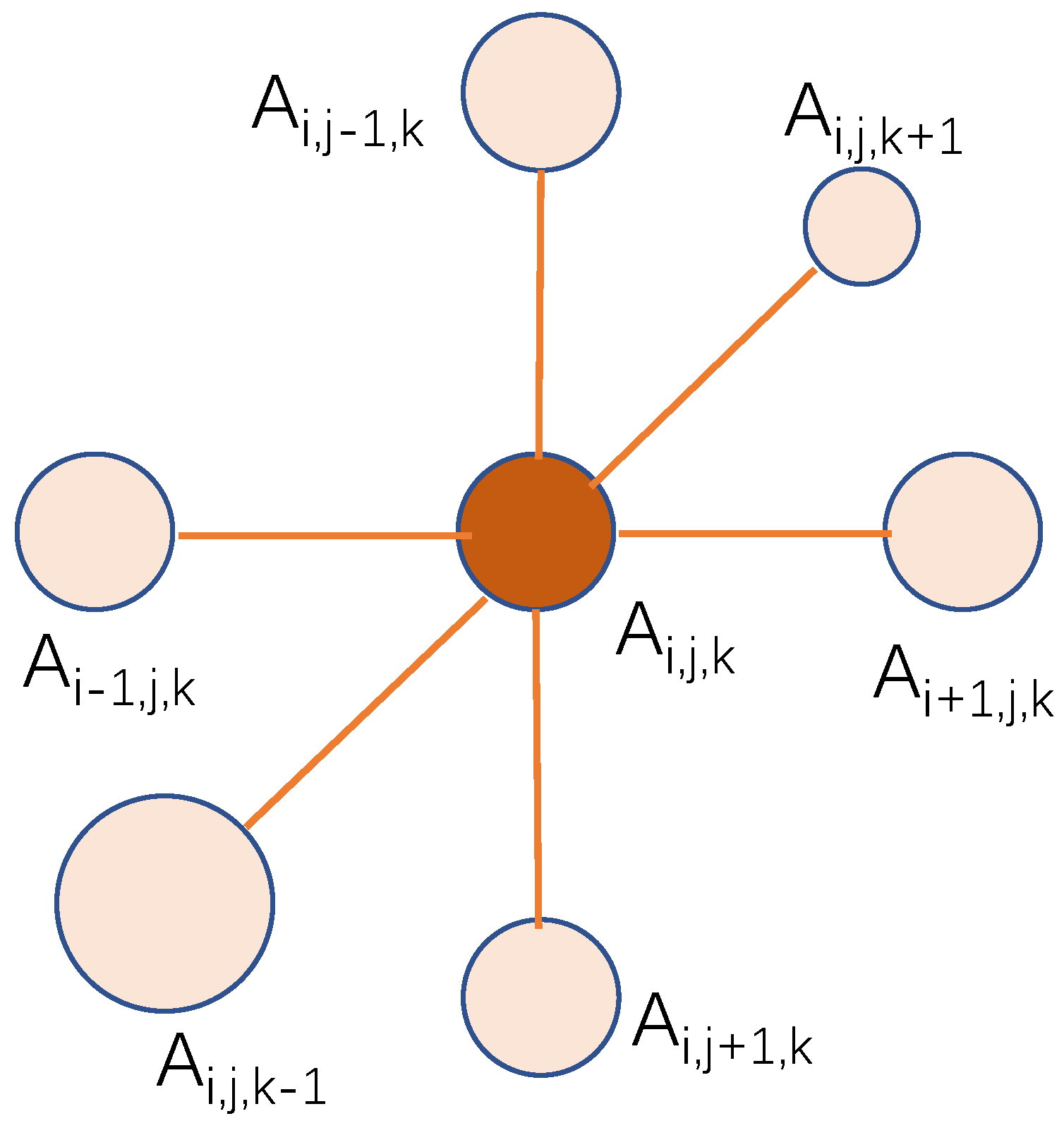
2.1. The Stencil Problem

As is described in Algorithm 1, the general computation pattern of stencil computation is that the central point accumulates the contributions of neighbor points in every axis of the Cartesian coordinate system; Figure 1 shows an example of 3D point stencil computation. The number of neighbor points in each axis or grid step of the stencil computation corresponds to the accuracy of the stencil. The more neighbor elements involved in the computation, the higher accuracy the computation obtains. The computation is then repeated for every point of the grid domain as an iterative operator of the PDEs.

It can be identified from the structure of the stencil computation that two inherent problems exist:

• First, it is the non-continuous memory access pattern. There exist distances among elements needed for the computation except those in the innermost or the unit-stride dimension. Many more cycles in latencies are required to access these points. Furthermore, much more costs are paid with a bigger stencil radius.
• Second, it is the low arithmetic intensity and poor data reuse. Just one point is updated with all the elements loaded. The data reuse between two updates is also limited within the unit-stride dimension, while the other dimensions’ elements that are expensive to access have no data reuse at all.

Algorithm 1 The classical stencil algorithm pseudo-code for a 3D problem [1]

Require:$A^t$, $A^{t-1}$, r, $z_s$, $z_e$, $y_s$, $y_e$, $x_s$, $x_e$; 1: Procedure STENCIL(); 2: for$k=z_s\to z_e$do 3:    for $j=y_s\to y_e$ do 4:      for $i=x_s\to x_e$ do 5:         $A_{i,j,k}^t=C_0\times A_{i,j,k}^{t-1}$          $+C_{x1}\times A_{i\pm 1,j,k}^{t-1}+\cdots +C_{xr}\times A_{i\pm r,j,k}^{t-1}$          $+C_{y1}\times A_{i,j\pm 1,k}^{t-1}+\cdots +C_{yr}\times A_{i,j\pm r,k}^{t-1}$          $+C_{z1}\times A_{i,j,k\pm 1}^{t-1}+\cdots +C_{zr}\times A_{i,j,k\pm r}^{t-1}$; 6:      end for 7:    end for 8: end for 9: End Procedure;

3. Transformation Optimizations Recipes

Loop transformation has long been a successful recipe in modern commodity compilers for a while. In this section, we investigate several transformation recipes and apply them to the optimizations of stencil computation.

3.1. Loop Unrolling

Loop unrolling [5,9,10] is most commonly used to reduce the loop overheads and provide instruction-level parallelism for processors with multiple functional units. It also facilitates the scheduling of the instruction pipeline. Since expansion can eliminate branches and some code that manages induction variables, some branching overhead can be amortized. These features effectively support expansion in any dimension, even in multiple dimensions. If used properly, it can increase reusability. However, excessive use of this technique can cause excessive register pressures and may reduce performance. Algorithm 2 shows an example of Stencil code for loop unrolling in the innermost loop with an unroll factor of uf.

Algorithm 2 Loop unrolling algorithm

Require:$A^t$, $A^{t-1}$, r, $z_s$, $z_e$, $y_s$, $y_e$, $x_s$, $x_e$, $uf$;  1: Procedure UNROLL();  2: for$k=z_s\to z_e$do  3:    for $j=y_s\to y_e$ do  4:      for $i=x_s\to x_e,uf$ do  5:         $update{A}_{i,j,k}^t$;  6:         ⋯;  7:         $update{A}_{i+uf-1,j,k}^t$;  8:      end for  9:    end for 10: end for 11: BoundaryProcessing(); 12: End Procedure;

3.2. Loop Fusion

Loop fusion [11,12] is another algorithm structure adjustment technique. The basic starting point is to change the data dependencies of the original stencil computation through the adjustment of the algorithm structure, improve the memory access footprint behavior, and then improve the performance. As is shown in Figure 2, between two different time steps, the original stencil computation memory footprint has periodic data dependencies: at a certain time step T, an element’s update requires the value of its neighbor elements at time T-1; conversely, the neighbor elements also need its neighbor elements at time T-2 to be updated. Generally, this dependency is avoided by writing the updated value of the element at the next time-step into a new array, and after the computation of the entire grid is completed, it is exchanged with the original array (or through pointer exchange, and data copy) to achieve continuous iteration. In this way, in addition to the original input array, an additional array with the same size as the original array has to be used.

To break this inherent dependency and develop parallelism without multiple copies of data, one needs to study the existing data dependency carefully. Back to Figure 2, in a single iteration of the 3D 7pt stencil computation, it can be seen that under the row-first storage pattern and the linear memory access mode, the elements required for the current computation are its continuous right neighbor elements. For the 7pt computation mode, since its radius is 1, the last one that requires element A0[k][j][i] is element A0[k+1][j][i]. One solution to eliminate the dependencies above is to create a temporary array to temporarily store the elements needed for the next iteration until the last element that needs them is updated. In this way, it is possible to update the element A0[k][j][i] in the original array A0 without the need for the Anext array. Algorithm 3 shows the pseudo-code of the above optimization scheme.

Algorithm 3 Loop fusion algorithm

Require:$A^t$, $A^{t-1}$, r, $z_s$, $z_e$, $y_s$, $y_e$, $x_s$, $x_e$, H, $tem{p}^t$, $tem{p}^{t-1}$;  1: Procedure FUSION();  2: for$k=z_s\to z_e$do  3:    for $j=y_s\to y_e$ do  4:      for $i=x_s\to x_e$ do  5:         if $i\ge H+1$ then  6:           $A_{i-H,j,k}^t=tem{p}_{(i-1)\%H,j,k}^t$;  7:         end if  8:         $tem{p}_{(i-1)\%H,j,k}^t=A_{i,j,k}^t$;  9:      end for 10:    end for 11: end for 12: End Procedure;

In the above algorithm, temp is the temporary array, and A is the original input array. H is the number of element planes that need to be temporarily stored, which is determined according to the radius of the stencil. Lines 5–7 of the pseudo-code indicate that after the dependency is eliminated, the data elements temporarily stored in temp can be rewritten back to array A. Line 8 indicates that the updated elements are temporarily stored in the array temp. It is worth noting that although the temp array is still of the same dimensions as the original input array, its scale is much smaller than the original input array. It only needs to contain several data planes at the outermost loop (depending on factors, such as the radius of the stencil computation mode). In this way, compared to the original implementation, data accesses are reduced by k/H times. While reducing the data access footprints, it also improves data locality.

3.3. Address Precalculation

Another fairly standard optimization technique is to precalculate the memory address in a nested loop [13]. Although the virtual address space is organized as one-dimensional (or linear), the data structure usually represents higher-dimensional fields. Multi-dimensional accesses must be linearized (as is shown in Algorithm 4). All accesses are eventually linearized, which reveals redundant computations and justifies the optimization. For example, linearizing the access of src[k][j][i] in the array (extending 512 elements in each dimension) produces an access to src[262144 * k + 512 * j + i]. If i is an iterator of the innermost loop, and y and z are not modified in the body of the innermost loop, there is no need to calculate the sub-expression 262,144 * k + 512 * j over and over again. It is sufficient to evaluate it once before the i cycle. Multiple accesses of adjacent elements of the same field share the same sub-expression and can be combined for optimization. In theory, commercial compilers can also eliminate some of these redundancies. However, combined with other transformations (such as vectorization), the generated code may become too complex, and there are still redundancies. Therefore, we directly implement such optimization to ensure that it is always applied.

3.3.1. Code Analysis

The main task of this strategy is to identify the sub-expressions that are not related to loops in the array index computation. It searches for a suitable loop and collects all array accesses and variables modified or declared in the loop body or header. The latter must stay inside the loop, and only sub-expressions that do not contain any of these variables can be moved outside. After fully traversing a loop and collecting all array accesses, its index computation is analyzed. Its summation items are divided into those precalculated ones and must stay in the loop. Even if a constant summation number can be added to the previous group, we should not do this. The following example illustrates why. A simple stencil calculates the center element and its immediate neighbors as shown in Algorithm 4. Applying the described partitions, the sum of all accesses that should be precalculated is the same, that is k: 262,144, j: 512, which generates a new base pointer for all accesses, as shown in Algorithm 5 (Line 4).

Algorithm 4 Original stencil code with linear array access

Require:$A^t$, $A^{t-1}$, $z_s$, $z_e$, $y_s$, $y_e$, $x_s$, $x_e$, $nx$, $ny$, $nz$; 1: Procedure LINEARACCESS(); 2: for$k=z_s\to z_e$do 3:    for $j=y_s\to y_e$ do 4:      for $i=x_s\to x_e$ do 5:         $A_{nx\ast ny\ast k+nx\ast j+i}^t=C_0\times A_{nx\ast ny\ast k+nx\ast j+i}^{t-1}$                       $+C_{x1}\times A_{nx\ast ny\ast k+nx\ast j+i\pm 1}^{t-1}$                       $+C_{y1}\times A_{nx\ast ny\ast k+nx\ast (j\pm 1)+i}^{t-1}$                       $+C_{z1}\times A_{nx\ast ny\ast (k\pm 1)+nx\ast j+i}^{t-1}$; 6:      end for 7:    end for 8: end for 9: End Procedure;

3.3.2. Integrate the Changes

A separate transformation is required to incorporate these changes because all the variables written in the loop body must be collected before the redundant sub-expression is determined. However, the previous collector is ready for new declarations and array accesses. In Algorithm 5, the only part remaining is to put these declarations before the corresponding loop (Line 4) and replace the array access (Line 6).

Algorithm 5 Stencil code with optimized index access

Require:$A^t$, $A^{t-1}$, P, $z_s$, $z_e$, $y_s$, $y_e$, $x_s$, $x_e$, $nx$, $ny$, $nz$;  1: Procedure OPTIMIZEDACCESS();  2: for$k=z_s\to z_e$do  3:    for $j=y_s\to y_e$ do  4:      $P\leftarrow A_{nx\ast ny\ast k+nx\ast j}^t$;  5:      for $i=x_s\to x_e$ do  6:         $P_i^t=C_0\times P_i^{t-1}$          $+C_{x1}\times P_{i\pm 1}^{t-1}$          $+C_{y1}\times P_{i\pm nx}^{t-1}$          $+C_{z1}\times P_{i\pm nx\ast ny}^{t-1}$;  7:      end for  8:    end for  9: end for 10: End Procedure;

3.4. Redundancy Elimination

Eliminating redundant computations [13] is an obvious way to improve performance. In several situations, redundant computations may occur. One method is explained in the previous section, namely, the precalculation of memory address computation. The general redundancy elimination described in this section is mainly aiming at the actual computation of the generated kernel and solves the redundancy within a single loop iteration and between loop iterations. The latter is particularly useful in the case of finite volume discretization.

Common subexpression elimination (CSE) [8] is often implemented in commercial compilers [14] (Figure 3 gives an example). The basic idea is to remove repeated computations from the expression by reusing the result of the previous computation. This optimization can only be applied if no associated variables or storage areas are modified between repeated evaluations of sub-expressions. The disadvantage is that CSE may increase register pressures because other values must be retained, which may cause register overflows. However, in this case, the assumption is that for larger expressions, newly introduced memory access operations are faster than expression recomputation. Algorithm 6 is the case of applying it to stencil computation.

Algorithm 6 Stencil computation with the principle of sub-expression elimination

Require:$A^t$, $A^{t-1}$, $z_s$, $z_e$, $y_s$, $y_e$, $x_s$, $x_e$, $temp1$, $temp2$;  1: Procedure CSE();  2: for$k=z_s\to z_e$do  3:    for $j=y_s\to y_e$ do  4:      for $i=x_s\to x_e,2$ do  5:         $temp1=C_0\times A_{i,j,k}^{t-1}$;  6:         $temp2=C_0\times A_{i+1,j,k}^{t-1}$;  7:         $A_{i,j,k}^t=temp1+C_{x1}/C_0\times temp2$                       $+C_{x1}\times A_{i-1,j,k}^{t-1}$                       $+C_{y1}\times A_{i,j\pm 1,k}^{t-1}$                       $+C_{z1}\times A_{i,j,k\pm 1}^{t-1}$;  8:         $A_{i+1,j,k}^t=temp2+C_{x1}/C_0\times temp1$                       $+C_{x1}\times A_{i+2,j,k}^{t-1}$                       $+C_{y1}\times A_{i+1,j\pm 1,k}^{t-1}$                       $+C_{z1}\times A_{i+1,j,k\pm 1}^{t-1}$;  9:      end for 10:    end for 11: end for 12: End Procedure;

3.5. Instruction Reordering

Register allocation is generally considered a practically solved problem [15]. For most applications, the register allocation strategy in the production compiler is very effective in controlling the number of loads/stores and register overflows. However, the existing register allocation strategy is ineffective and causes numerous registers to overflow, resulting in computation modes with high many-to-many data reuses, such as high-level stencils and tensor contractions [15]. This strategy takes advantage of the flexibility of reordering associated operations to reduce register pressure. This strategy can appropriately control the instruction-level parallelism while reducing the pressure on registers. All in all, this reorder method can firstly reduce the register pressure in a single loop, such as a reorder of the codes with an unroll factor of 2; second, it can improve data locality.

In the reordering computation, the evaluation of different output points is interleaved so that all the uses of an input value are closer, thus shortening its effective range. This method can be migrated to the cache level, not only for registers. Through the appropriate combination and allocation of multiplication, addition, and division, it can also improve the data reuse and locality of the cache levels.

The process of computation reordering is given below in conjunction with the 3D 7pt stencil algorithm. As is shown in Algorithm 7, we first expand the original Formulas (2) and (3) into Formulas (6)–(11):

Algorithm 7 Expand the 2 original iteration formulas

Require:$A^t$, $A^{t-1}$, $z_s$, $z_e$, $y_s$, $y_e$, $x_s$, $x_e$;  1: Procedure ORIGIN();  2: $A_{i,j,k}^t=C_0\times A_{i,j,k}^{t-1}$       $+C_{x1}\times (A_{i-1,j,k}^{t-1}+A_{i+1,j,k}^{t-1})$       $+C_{y1}\times (A_{i,j-1,k}^{t-1}+A_{i,j+1,k}^{t-1})$       $+C_{z1}\times (A_{i,j,k-1}^{t-1}+A_{i,j,k+1}^{t-1})$;  3: $A_{i+1,j,k}^t=C_0\times A_{i+1,j,k}^{t-1}$       $+C_{x1}\times (A_{i,j,k}^{t-1}+A_{i+2,j,k}^{t-1})$       $+C_{y1}\times (A_{i+1,j-1,k}^{t-1}+A_{i+1,j+1,k}^{t-1})$       $+C_{z1}\times (A_{i+1,j,k-1}^{t-1}+A_{i+1,j,k+1}^{t-1})$;  4: End Procedure;  5: Procedure EXPAND1();  6: $A_{i,j,k}^t=C_0\times A_{i,j,k}^{t-1}$       $+C_{x1}\times (A_{i-1,j,k}^{t-1}+\times A_{i+1,j,k}^{t-1})$;  7: $A_{i+1,j,k}^t=C_0\times A_{i+1,j,k}^{t-1}$       $+C_{x1}\times (A_{i,j,k}^{t-1}+A_{i+2,j,k}^{t-1})$;  8: $A_{i,j,k}^t+=C_{y1}\times (A_{i,j-1,k}^{t-1}+\times A_{i,j+1,k}^{t-1})$;  9: $A_{i+1,j,k}^t+=C_{y1}\times (A_{i+1,j-1,k}^{t-1}+A_{i+1,j+1,k}^{t-1})$; 10: $A_{i,j,k}^t+=C_{z1}\times (A_{i,j,k-1}^{t-1}+\times A_{i,j,k+1}^{t-1})$; 11: $A_{i+1,j,k}^t+=C_{z1}\times (A_{i+1,j,k-1}^{t-1}+A_{i+1,j,k+1}^{t-1})$; 12: End Procedure;

The first two lines (lines 6–7) reuse $A_{i,j,k}^{t-1}$ and $A_{i+1,j,k}^{t-1}$, and use the i-dimension locality to access $A_{i-1,j,k}^{t-1}$ and $A_{i+2,j,k}^{t-1}$. The next line (line 8) accesses $A_{i,j-1,k}^{t-1}$ and $A_{i,j+1,k}^{t-1}$ first, and then uses the i-dimensional locality to visit $A_{i+1,j-1,k}^{t-1}$ and $A_{i+1,j+1,k}^{t-1}$ respectively. Lines 10–11 behave in a similar pattern in the z-dimension. One can also continue to expand, and expand more finely (not more than 2 operands at a time), that is, expand the original Formulas (2) and (3) in Algorithm 7 into Formulas (2)–(15) in Algorithm 8. The final computation process is shown in Algorithm 8:

Algorithm 8 Continue to expand the formula in Algorithm 7

Require:$A^t$, $A^{t-1}$, $z_s$, $z_e$, $y_s$, $y_e$, $x_s$, $x_e$;  1: Procedure EXPAND2();  2: $A_{i,j,k}^t=C_{x1}\times A_{i-1,j,k}^{t-1}$;  3: $A_{i,j,k}^t+=C_0\times A_{i,j,k}^{t-1}$;  4: $A_{i+1,j,k}^t+=C_{x1}\times A_{i,j,k}^{t-1}$;  5: $A_{i,j,k}^t+=C_{x1}\times A_{i+1,j,k}^{t-1}$;  6: $A_{i+1,j,k}^t+=C_0\times A_{i+1,j,k}^{t-1}$;  7: $A_{i+1,j,k}^t+=C_{x1}\times A_{i+2,j,k}^{t-1}$;  8: $A_{i,j,k}^t+=C_{y1}\times A_{i,j-1,k}^{t-1}$;  9: $A_{i+1,j,k}^t+=C_{y1}\times A_{i+1,j-1,k}^{t-1}$; 10: $A_{i,j,k}^t+=C_{y1}\times A_{i,j+1,k}^{t-1}$; 11: $A_{i+1,j,k}^t+=C_{y1}\times A_{i+1,j+1,k}^{t-1}$; 12: $A_{i,j,k}^t+=C_{z1}\times A_{i,j,k-1}^{t-1}$; 13: $A_{i+1,j,k}^t+=C_{z1}\times A_{i+1,j,k-1}^{t-1}$; 14: $A_{i,j,k}^t+=C_{z1}\times A_{i,j,k+1}^{t-1}$; 15: $A_{i+1,j,k}^t+=C_{z1}\times A_{i+1,j,k+1}^{t-1}$; 16: End Procedure;

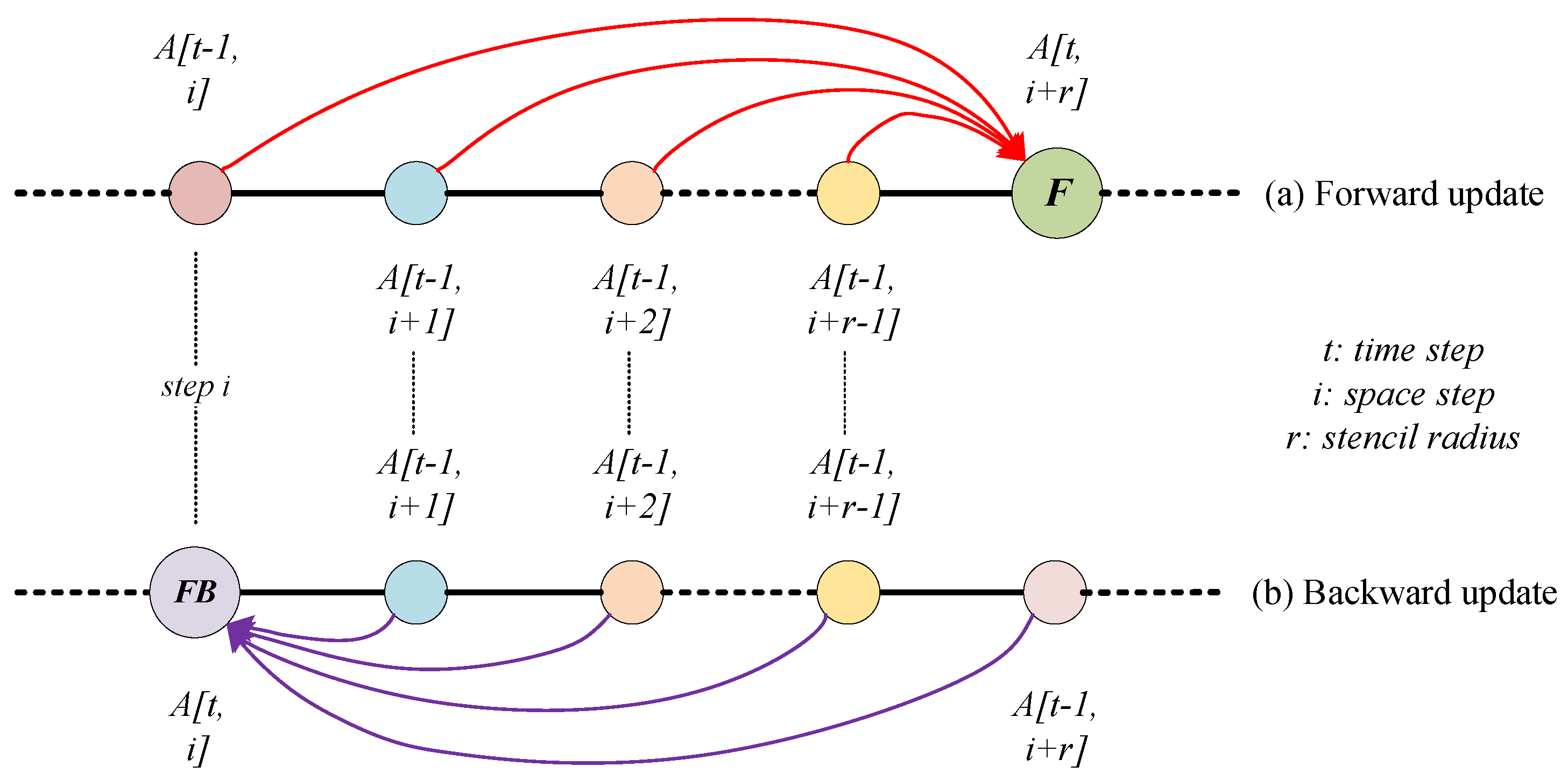
3.6. Forward and Backward Update Algorithm

As is mentioned above, the stencil computation tends to be memory bound and has a low computation to memory access ratio. It is used to solve the problem that [1,16] put forward the semi-stencil algorithm. We introduce the algorithm’s main idea in brief and provide an analysis of its effect on the arithmetic intensity.

3.6.1. Forward and Backward Updates

The semi-stencil algorithm employs a new memory access pattern for the original stencil computation by altering its structure. The new algorithm structure consists of two phases: forward update and backward update, which are described in Figure 4 for a 1D stencil instance.

The forward update is the first contributions that point A[i+r] at time step t receives (as depicted in Figure 4a). In this phase, the point $A_{i+r}^t$ is updated with its r rear neighbors at time step t− 1, i.e., points $A_{i,...,i+r-1}^{t-1}$. The forward update can be summarized, in mathematical terms, as

$$\begin{array}{c}\hfill A_{i+r}^{{}^{\prime }t}=C_1\times A_{i+r-1}^{t-1}+C_2\times A_{i+r-2}^{t-1}\\ \hfill +\cdots \\ \hfill +C_{r-1}\times A_{i+1}^{t-1}+C_r\times A_i^{t-1}\end{array}$$

(1)

where the prime character (${}^{\prime }$) denotes that the point is only partially updated, and some contributions are still missing [1]. Note that we load r elements, i.e., points $A_{i,...,i+r-1}^{t-1}$, in Formula (1), and only one element, $A_{i+r}^{{}^{\prime }t}$, is stored.

As for the second phase, named backward update, the pre-updated point $A_i^t$ in the forward phase is completed by adding the rest of the contributions in the original stencil computation, i.e., points $A_{i,...,i+r}^{t-1}$. To be specific,

$$\begin{array}{c}\hfill A_i^t=A_i^{{}^{\prime }t}+C_0\times A_i^{t-1}+C_1\times A_{i+1}^{t-1}+C_2\times A_{i+2}^{t-1}\\ \hfill +\cdots \\ \hfill +C_{r-1}\times A_{i+r-1}^{t-1}+C_r\times A_{i+r}^{t-1}\end{array}$$

(2)

What is noted is that only two more loads are required in the backward phase, i.e., point $A_{i+r}^{t-1}$ and the pre-updated value $A_i^{{}^{\prime }t}$. The rest of the points required are loaded during the forward phase at time step t-1 for the update of $A_{i+r}^t$ computation. One additional store to write back the final updated value, $A_i^t$, is also needed.

To carry out the two-phase update algorithm, the original factored add and mul operations ($C_i\times (A_{-i}+A_i)$) must be decomposed into multiply–add instructions ($C_i\times A_{-i}+C_i\times A_i$) to split up the original computation into a forward and a backward phase.

3.6.2. Arithmetic Intensity Analysis

We compare the arithmetic intensities of the original stencil computation and the altered stencil computation with the semi-stencil algorithm. As is depicted in Section 2.1, the arithmetic intensity or floating-point operations to data access ratio of the original classical stencil computation is

$$\begin{array}{cc}\hfill A{I}_{classical}& =\frac{FloatingPointOperations}{DataAccesses}\hfill \\ \hfill & =\frac{\#ADD+\#MUL}{\#Loads+\#Stores}\hfill \\ \hfill & =\frac{2\times 2\times dim\times r+1}{2\times (dim-1)\times r+1+1}\hfill \\ \hfill & =\frac{4\times dim\times r+1}{2\times r\times (dim-1)+2}\hfill \end{array}$$

(3)

As for the altered stencil computation with the semi-stencil algorithm, the $A{I}_{fb}$ is

$$\begin{array}{cc}\hfill A{I}_{fb}& =\frac{FloatingPointOperations}{DataAccesses}\hfill \\ \hfill & =\frac{\#ADD+\#MUL}{\#Loads+\#Stores}\hfill \\ \hfill & =\frac{2\times 2\times dim\times r+1}{(dim-1)\times r+1+dim-1+dim}\hfill \\ \hfill & =\frac{4\times dim\times r+1}{dim\times r-r+2\times dim}\hfill \end{array}$$

(4)

It can be observed that they have the same FloatingPointOperations, while the altered stencil computation with the semi-stencil algorithm has a lower number of loads and stores due to the reuse of elements between the forward and backward phases. It can be induced that $A{I}_{fb}\ge A{I}_{classical}$ when $r\ge 2$, which means the semi-stencil algorithm has a better cache reuse behavior.

3.7. Load Balance

It is the balanced combination of floating-point operations [17]. Optimal performance requires that a large part of the instruction mix is floating-point operations. Peak floating-point performance usually also requires equal numbers of simultaneous floating point additions and multiplications because many computers have multiply–add instructions or equal numbers of adders and multipliers. Specifically, for a stencil computation, it is good choice to expand the multiplication factor according to the associative law of addition, as is shown in Algorithm 9.

Algorithm 9 Stencil computation with load balance

Require:$A^t$, $A^{t-1}$, $z_s$, $z_e$, $y_s$, $y_e$, $x_s$, $x_e$; 1: Procedure BALANCE(); 2: for$k=z_s\to z_e$do 3:    for $j=y_s\to y_e$ do 4:      for $i=x_s\to x_e$ do 5:         $A_{i,j,k}^t=C_0\times A_{i,j,k}^{t-1}$          $+C_{x1}\times A_{i-1,j,k}^{t-1}+C_{x1}\times A_{i+1,j,k}^{t-1}$          $+C_{y1}\times A_{i,j-1,k}^{t-1}+C_{y1}\times A_{i,j+1,k}^{t-1}$          $+C_{z1}\times A_{i,j,k-1}^{t-1}+C_{z1}\times A_{i,j,k+1}^{t-1}$; 6:      end for 7:    end for 8: end for 9: End Procedure;

3.8. Put It All Together

It is worth noting that the above optimization options are not isolated from each other. They can be appropriately combined, and then performance testing and analysis of the combined optimization options can be performed.

4. Experimental Evaluations

In this section, the evaluation results of the various recipes are presented. The benchmarks utilized are introduced firstly in brief. Second, we describe the experimental platforms to conduct related tests. The performance improvements of the separate transformation recipes are then analyzed finally.

4.1. Stencil Benchmarks

To evaluate the performance of our proposed recipes for stencil computation, the following stencil instances listed in

Table 1. List of parameters employed for the extended version of the classical stencil.

Parameters	Range of Values
Problem sizes	16 M, 32 M, 64 M (1D), $8K^2$, $16K^2$, $32K^2$ (2D) ${128}^3$, ${256}^3$, ${512}^3$, ${1024}^3$ (3D)
Stencil sizes(r)	1, 2, 4, 5, 7, 14
Stencil	1D 3pt, 1D 11pt, 2D 5pt, 2D 121pt, 3D 7pt, 3D 13pt, 3D 25pt, 3D 27pt, 3D 43pt, 3D 85pt, 3D 125pt Jacobi
Time-steps	1, 100
Algorithms	naive, loop unroll, loop fusion, address precalculation redundancy elimination, instruction reordering semi-stencil, load balance, compound recipes

are employed to test the floating-point performance. For the dimension of stencils, 1D, 2D, and 3D stencils are all developed. The problem sizes also range from 16 M to 64 M for 1D stencils, 8K × 8K to 32K× 32K for 2D stencils, and 128 × 128 × 128 to 1024 × 1024 × 1024 for 3D ones. As for the time steps of the iteration, we both utilize one single step and one hundred steps. The diverse stencil radii of $\mathit{r}=1,2,4,5,7,14$ are coded for the forward and backward update algorithm. It is worth noting that not all the parameters listed are set for all the stencil instances. One reason is that the stencil features may vary according to the instances. The other is that the parameter space tends to be quite large to explore with all the configurations taking into consideration.

4.2. Testbed Architectures

The following two leading platforms described in

Table 2. Architectural summary of experimental platforms.

Core Architecture
Type	superscalar out-of-order	superscalar out-of-order
SIMD	NEON	AVX
Threads/Core	1	1
Clock (GHz)	2.2-2.4	2.4
DP (GFlops)	8.8	19.2
L1 Cache (D + I)	32 KB + 32 KB	32 KB + 32 KB
Socket Architecture
Cores/Socket	4	10
L2 Data Cache	2 MB/4 Cores	256 KB
Shared L3 Data Cache	-	25 MB
primary memory parallelism paradigm	HW prefetch	HW prefetch
System Architecture
Sockets/SMP	2	1
DP (GFlops)	563.2 @ 2.2 GHz	384
DRAM BW (GB/s)	204.8	68.3
DP Flop: Byte Ratio	2.75	5.62
DRAM Capacity (GB)	256	64
DRAM Type	DDR4-2666	DDR4-2133
System Power (W)	100	90
Compiler	gcc 8.3	gcc 4.8

are used to carry out the experiments.

• Intel Xeon E5: Intel Xeon CPU E5-2640 v4 @ 2.40 GHz, with 20 physical cores divided into 2 NUMA nodes, and AVX supported.
• ARM: ARMv8 ISA64 compatible processors, with 64 physical cores in total and evenly divided into 8 NUMA nodes, and SIMD Extension NEON supported [18].

4.3. Results and Analysis

As is presented in

Table 3. Experimental results of the proposed transformation recipes: (e) loop fusion (ARM).

3D 7pt	N	Naive	Fusion	Speedup
T = 1	128	1.15	1.15	1.00
T = 100		1.46	1.18	0.81
T = 1	256	1.23	0.91	0.74
T = 100		1.56	0.92	0.58
T = 1	512	0.94	0.79	0.84
T = 100		1.13	0.80	0.70
2D 5pt	N	naive	fusion	Speedup
T = 1	8K	0.63	0.74	1.17
T = 100		0.76	0.75	0.99
T = 1	16K	0.60	0.62	1.02
T = 100		0.73	0.62	0.85
T = 1	32K	0.53	0.47	0.87
T = 100		0.64	0.46	0.73
1D 3pt	N	naive	fusion	Speedup
T = 1	16M	0.89	0.57	0.64
T = 100		1.67	0.57	0.34
T = 1	32M	0.90	0.55	0.61
T=100		1.66	0.55	0.33
T = 1	64M	0.90	0.53	0.59
T = 100		1.66	0.53	0.32

,

Table 4. Experimental results of the proposed transformation recipes: (f) loop fusion (Intel).

3D-7pt	N	Naive	Fusion	Speedup
T = 1	128	2.03	3.83	1.88×
T = 100		4.20	4.34	1.03×
T = 1	256	2.57	3.74	1.45×
T = 100		4.05	3.75	0.92×
T = 1	512	2.48	3.67	1.48×
T = 100		3.89	3.67	0.94×
2D-5pt	N	naive	fusion	Speedup
T = 1	8K	1.68	2.46	1.45×
T = 100		2.57	2.45	0.95×
T = 1	16K	1.61	2.39	1.48×
T = 100		2.40	2.39	0.99×
T = 1	32K	1.35	2.39	1.76×
T = 100		2.08	2.13	1.02×
1D-3pt	N	naive	fusion	Speedup
T = 1	16M	1.03	0.79	0.76×
T = 100		1.67	0.79	0.47×
T = 1	32M	1.04	0.79	0.75×
T = 100		1.66	0.80	0.48×
T = 1	64M	1.02	0.81	0.79×
T = 100		1.69	0.81	0.48×

,

Table 5. Experimental results of the proposed transformation recipes: (g) forward and backward algorithm (ARM).

N	Version	r = 1		r = 2		r = 4		r = 7		r = 14
		GFs.	Spe.	GFs.	Spe.	GFs.	Spe.	GFs.	Spe.	GFs.	Spe.
128	naive	1.85	1.00×	2.52	1.00×	1.55	1.00×	1.16	1.00×	1.17	1.00×
	fb	1.45	0.78×	2.16	0.86×	1.62	1.05×	1.38	1.19×	1.79	1.53×
256	naive	1.96	1.00×	1.62	1.00×	1.44	1.00×	0.95	1.00×	0.83	1.00×
	fb	1.47	0.75×	1.48	0.91×	1.45	1.01×	1.09	1.15×	1.41	1.70×
512	naive	1.41	1.00×	1.99	1.00×	1.32	1.00×	1.00	1.00×	0.75	1.00×
	fb	0.55	0.39×	1.71	0.86×	1.45	1.10×	1.07	1.07×	1.20	1.60×
1024	naive	0.84	1.00×	1.61	1.00×	1.40	1.00×	0.93	1.00×	0.69	1.00×
	fb	0.82	0.98×	1.11	0.69×	1.43	1.02×	0.92	0.99×	1.06	1.52×

and

Table 6. Experimental results of the proposed transformation recipes: (h) forward and backward algorithm (Intel).

N	Version	r = 1		r = 2		r = 4		r = 7		r = 14
		GFs.	Spe.	GFs.	Spe.	GFs.	Spe.	GFs.	Spe.	GFs.	Spe.
128	naive	4.73	1.00×	5.84	1.00×	2.37	1.00×	2.18	1.00×	2.52	1.00×
	fb	3.19	0.68×	4.12	0.71×	2.91	1.23×	2.13	0.98×	2.77	1.10×
256	naive	5.06	1.00×	5.66	1.00×	2.27	1.00×	1.73	1.00×	1.76	1.00×
	fb	3.17	0.63×	4.05	0.72×	2.68	1.18×	1.82	1.05×	1.95	1.10×
512	naive	2.44	1.00×	3.96	1.00×	2.04	1.00×	1.74	1.00×	1.15	1.00×
	fb	1.48	0.61×	3.76	0.95×	2.36	1.16×	1.69	0.97×	1.70	1.47×
1024	naive	2.56	1.00×	3.60	1.00×	1.88	1.00×	1.59	1.00×	1.06	1.00×
	fb	1.99	0.78×	2.81	0.78×	1.94	1.03×	1.59	1.00×	1.54	1.45×

, both the single transformation recipe and compound recipes results are provided. These tables show the floating-point performance for the stencils and the relative improvements compared to the naive implementations. The address precalculation and redundancy elimination recipes do not apply to the 1D stencils.

Loop unrolling. The best performance improvement of 1.65× is obtained for the 2D 5pt stencil with an unrolling factor of 2. The average speedup of all the benchmarks analyzed is 1.18×. Notably, there is a parameter space for this unrolling recipe: multi-dimensions exist, and the unrolling factor can vary according to the number of registers on a specific architecture and the points involved in a stencil computation.

When it comes to Intel, however, a diverse phenomenon occurs. Hardly any performance improvement is obtained. It is true for both the single recipe and compound recipes results from Figure 5, Figure 6, Figure 7 and Figure 8. We attribute this to the compiler optimization strategies’ differences and optimization options’ variances of diverse versions [19,20].

Loop fusion. On Intel, the best benefit is 1.88× at 3D 7pt with a single time-step. It can be seen that under a single time step, for the ×86 platform, 2D and 3D stencil computations show good acceleration effects. For 1D stencil computation, the advantages of this method are not reflected. Under multiple time steps, this data dependency is not well eliminated, and performance is not dramatically improved.

As is demonstrated in Table 3, when it comes to ARM, we did not obtain the expected acceleration effects. Further analysis shows that the ARM platform uses the so-called write-streaming mechanism. When writing back an array, it does not write it to the memory through the cache but uses a write-through strategy. It directly writes the relevant data, which need to be written back to the memory in the form of streaming data access. In other words, in the writing-stream mode, the loading behavior is normal and may still cause line splits. Writes still lookup in the cache, but if they miss, then they write out to L2 or L3 or L4 rather than starting a linefill. The above optimizations made for the write-back array do not work as expected.

Address precalculation. When it comes to the address precalculation recipe, not much improvement is observed among all the benchmarks investigated. One of the reasons may be that the GCC compiler integrates such a technique or the overhead of address computations is too small. However, we acquire the best speedup of 1.57× at 2D 5pt stencil.

Redundancy elimination. As to the redundancy elimination recipe, an average of 1.20× and the best improvement of 1.45× are acquired.

Instruction reordering. Poor performance improvements occur for all the benchmarks employed when investigating the instruction reordering recipe. One main cause of this phenomenon may be that the stencils we consider are of simple structures without many related benefits to be explored.

FB algorithm. In the forward and backward algorithm, five stencil radii of $\mathit{r}=1,2,4,7,14$ are coded, as is shown in Table 5 and Table 6. As is analyzed above, the stencil radius has a significant effect on the data reuse and arithmetic intensity of the stencil computation pattern. The bigger stencil radius implies a better improvement of this specific algorithm. On ARM, a speedup of 1.70× is obtained at r = 14 (a 3D-85pt stencil) for an input grid domain of 256 × 256 × 256. Similar results are observed on Intel, with the best improvement of $1.47\times$ at $r=14$ (a 3D 85pt stencil) for an input grid domain of 512 × 512 × 512.

Compound recipes. In Figure 7, p stands for address precalculation strategy, e stands for redundancy elimination strategy, u stands for loop unrolling strategy, and b stands for the load balance recipe. A combination of the above-mentioned transformation recipes presents excellent improvement behavior. To be specific, a combination of address precalculation and redundancy elimination (p.e.) presents a 1.27× performance improvement. A speedup of 1.92× is obtained by combining three recipes (p.e.u). The p.e.b. combination demonstrates a 1.62× speedup over the naive version. By the p.e.u.b. recipe, we implement a 1.79× speedup.

5. Related Work

It is no doubt that compiler optimization techniques incorporated in production compilers are of vital significance. Meanwhile, interests in the optimizations of stencil computations are not new. Many remarkable techniques [9,10,13,21,22,23,24] were put forward in the previous decades. Refs. [25,26] described a high-level description of code transformations that serve as an interface to describe the composition of complex code transformations. How the interface is designed for both compiler developers and application/library developers is discussed. Better performance than manually-tuned codes is obtained. Refs. [27,28] proposed a model-guided empirical optimization framework in which techniques including splitting, fusion and distribution, permutation, unroll-and-jam, tiling, and data copy are studied on matrix vector and matrix multiply. Ref. [4] performed similar work. Ref. [29] presented an embedded scripting language, POET, which can be embedded within an arbitrary programming language, and support efficient parameterization of general code transformations produced either by compilers or by professional programmers. It significantly reduced the empirical tuning time of otherwise using a sophisticated source-code optimizer. Ref. [30] conducted similar work. Other works, such as [6,7,31], described general frameworks to represent loop transformations or put forward new approaches to transformations for general loop nests and stencils. ExaStencils [32] is such a project of which the central goal is to develop a radically new software technology for applications with exascale performance. The domain chosen by the project is stencil codes, especially the compute-intensive ones. The software technology developed in ExaStencils tries to facilitate the highly automatic generation of a large variety of efficient implementations via the judicious use of domain-specific knowledge in each sequence of optimization steps such that, in the end, exascale performance results are obtained.

Our work is a new trail and a combination of stencils and loop transformations. We made an effort to test the traditional transformation recipes on stencil computations and illustrate the possible benefits that may exist. The goal of our LOOPI project is to accomplish an automatic optimization framework for arbitrary stencils. In other words, the user of the framework does not consider the specific architectural details after defining the stencil patterns they concern, which is of great relief for programmers in the tedious tuning and optimizing process.

6. Conclusions and Future Work

In this paper, we investigated the optimization recipes for loop transformations. For the past decades, loop transformations have been integrated successfully into compilers as standard configurations. Some traditional recipes, such as loop unrolling, were set as default optimizations by many commodity compilers. However, the effects they have upon stencil computations are unknown, although they may behave well on many loop kernels. Our work is an effort to explore the potential benefits these recipes may bring to the stencil computations. Unsurprisingly, not all the recipes we considered in this work benefit the stencil computations.

References

1. Cruz, R.D.L.; Araya-Polo, M. Algorithm 942: Semi-Stencil. ACM Trans. Math. Softw. 2014, 40, 1–39. [Google Scholar] [CrossRef]
2. OLCF Titan Summit 2011. Available online: https://www.olcf.ornl.gov/event/titan2011 (accessed on 9 October 2021).
3. Diede, T.; Hagenmaier, C.F. The Titan Graphics Supercomputer architecture. Computer 1988, 21, 13–30. [Google Scholar] [CrossRef]
4. Bacon, D.F.; Graham, S.L.; Sharp, O.J. Compiler Transformations for High-Performance Computing. ACM Comput. Surv. 1994, 26, 345–420. [Google Scholar] [CrossRef] [Green Version]
5. Banerjee, U. Loop Transformations for Restructuring Compilers: The Foundations; Springer: Berlin/Heidelberg, Germany, 1993. [Google Scholar]
6. Sarkar, V.; Thekkath, R. A general framework for iteration-reordering loop transformations. ACM Sigplan Not. 1992, 27, 175–187. [Google Scholar] [CrossRef]
7. Wolf, M.E.; Lam, M.S. A Loop Transformation Theory and an Algorithm to Maximize Parallelism; IEEE Press: Piscataway, NJ, USA, 1991. [Google Scholar]
8. Cocke, J. Global common subexpression elimination. ACM Sigplan Not. 1970, 5, 20–24. [Google Scholar] [CrossRef]
9. Armejach, A.; Caminal, H.; Cebrian, J.M.; Langarita, R.; González-Alberquilla, R.; Adeniyi-Jones, C.; Valero, M.; Casas, M.; Moretó, M. Using Arm’s scalable vector extension on stencil codes. J. Supercomput. 2019, 76, 2039–2062. [Google Scholar] [CrossRef]
10. Armejach, A.; Caminal, H.; Cebrian, J.M.; González-Alberquilla, R.; Adeniyi-Jones, C.; Valero, M.; Casas, M.; Moretó, M. Stencil codes on a vector length agnostic architecture. In Proceedings of the 27th International Conference on Parallel Architectures and Compilation Techniques, Portland, OR, USA, 9–13 September 2018; pp. 1–12. [Google Scholar]
11. Manjikian, N.; Abdelrahman, T.S. Fusion of loops for parallelism and locality. Parallel Distrib. Syst. IEEE Trans. 1997, 8, 193–209. [Google Scholar] [CrossRef]
12. Kennedy, K.; Mckinley, K.S. Maximizing Loop Parallelism and Improving Data Locality via Loop Fusion and Distribution. In Languages & Compilers for Parallel Computing; Springer: Berlin/Heidelberg, Germany, 1994. [Google Scholar]
13. Stefan, K. Automatic Performance Optimization of Stencil Codes. Ph.D. Thesis, Universität Passau, Passau, Germany, 2020. [Google Scholar]
14. Aho, A.V.; Lam, M.S.; Sethi, R.; Ullman, J.D. Compilers: Principles, Techniques, and Tools, 2nd ed.; Addison-Wesley Longman Publishing Co., Inc.: Boston, MA, USA, 2006. [Google Scholar]
15. Rawat, P.S.; Rajam, A.S.; Rountev, A.; Rastello, F.; Sadayappan, P. Associative Instruction Reordering to Alleviate Register Pressure. In Proceedings of the SC18: International Conference for High Performance Computing, Networking, Storage and Analysis, Dallas, TX, USA, 11–16 November 2018; IEEE: Piscataway, NJ, USA, 2018. [Google Scholar]
16. de la Cruz, R.; Arayapolo, M.; Cela, J.M. Introducing the Semi-Stencil Algorithm; Springer: Berlin/Heidelberg, Germany, 2009. [Google Scholar]
17. Williams, S.; Waterman, A.; Patterson, D.A. Roofline: An insightful visual performance model for multicore architectures. Commun. ACM 2009, 52, 65–76. [Google Scholar] [CrossRef]
18. JianBin, F.; XiangKe, L.; Chun, H.; De Zun, D. Performance Evaluation of Memory-Centric ARMv8 Many-Core Architectures: A Case Study with Phytium 2000+. J. Comput. Sci. Technol. 2021, 36, 33–43. [Google Scholar]
19. GCC, the GNU Compiler Collection. Available online: https://www.gnu.org/software/gcc/libstdc++/ (accessed on 12 June 2021).
20. Using the GNU Compiler Collection (GCC). Available online: https://gcc.gnu.org/onlinedocs/gcc/Optimize-Options.html#Optimize-Options (accessed on 20 October 2020).
21. Bassetti, F.; Davis, K.; Quinlan, D.J. Optimizing Transformations of Stencil Operations for Parallel Object-Oriented Scientific Frameworks on Cache-Based Architectures. In Proceedings of the International Symposium on Computing in Object-Oriented Parallel Environments, Santa Fe, NM, USA, 8–11 December 1998; IEEE: Piscataway, NJ, USA, 1998. [Google Scholar]
22. Yun, Z. Towards Automatic Compilation for Energy Efficient Iterative Stencil. Ph.D. Thesis, Colorado State University, Fort Collins, CO, USA, 2016. [Google Scholar]
23. Seyfari, Y.; Lotfi, S.; Karimpour, J. Optimizing inter-nest data locality in imperfect stencils based on loop blocking. J. Supercomput. 2018, 74, 5432–5460. [Google Scholar] [CrossRef]
24. Donglin, C.; Jianbin, F.; Chuanfu, X.; Shizhao, C.; Zheng, W. Optimizing Sparse Matrix-Vector Multiplications on An ARMv8-based Many-Core Architecture. Int. J. Parallel Program. 2019, 48, 418–432. [Google Scholar]
25. Hall, M.; Chame, J.; Chen, C.; Shin, J.; Rudy, G.; Khan, M.M. Loop Transformation Recipes for Code Generation and Auto-Tuning; Springer: Berlin/Heidelberg, Germany, 2009. [Google Scholar]
26. Hall, M.W.; Chame, J.N.; Chen, C.; Shin, J.; Rudy, G.; Khan, M. Loop transformation recipes for code generation and auto-tuning. In Proceedings of the International Workshop on Languages and Compilers for Parallel Computing, Newark, DE, USA, 8–10 October 2009; IEEE: Piscataway, NJ, USA, 2009. [Google Scholar]
27. Hall, M. Model-Guided Empirical Optimization for Memory Hierarchy. Available online: https://dl.acm.org/doi/10.5555/1329582 (accessed on 9 October 2021).
28. Chen, C.; Shin, J.; Kintali, S.; Chame, J.; Hall, M. Model-Guided Empirical Optimization for Multimedia Extension Architectures: A Case Study. In Parallel and Distributed Processing Symposium; IEEE: Piscataway, NJ, USA, 2007. [Google Scholar]
29. Yi, Q.; Seymour, K.; You, H.; Vuduc, R.W.; Quinlan, D.J. POET: Parameterized Optimizations for Empirical Tuning. In Proceedings of the 21th International Parallel and Distributed Processing Symposium (IPDPS 2007), Long Beach, CA, USA, 26–30 March 2007. [Google Scholar]
30. István, Z. Reguly, Gihan R. Mudalige, M.B.G. Loop Tiling in Large-Scale Stencil Codes at Run-Time with OPS. IEEE Trans. Parallel Distrib. Syst. 2018, 4, 873–886. [Google Scholar]
31. Basu, P.; Hall, M.; Williams, S.; Straalen, B.V.; Oliker, L.; Colella, P. Compiler-Directed Transformation for Higher-Order Stencils. In Proceedings of the 2015 IEEE International Parallel and Distributed Processing Symposium, Hyderabad, India, 25–29 May 2015; IEEE: Piscataway, NJ, USA, 2015. [Google Scholar]
32. Advanced Stencil-Code Engineering (ExaStencils). Available online: https://www.exastencils.fau.de/ (accessed on 6 September 2021).
Figure 1. Examples of 3D point stencil.
Electronics 11 00038 g001
Figure 2. Footprints of a 3D Stencil under linear expression of memory space.
Electronics 11 00038 g002
Figure 3. Code example sub-expression elimination principle.
Electronics 11 00038 g003
Figure 4. Detail of the two phases for the semi-stencil algorithm at step i.
Electronics 11 00038 g004
Figure 5. Experimental results of the proposed transformation recipes: (a) single recipe (ARM).
Electronics 11 00038 g005
Figure 6. Experimental results of the proposed transformation recipes: (b) single recipe (Intel).
Electronics 11 00038 g006
Figure 7. Experimental results of the proposed transformation recipes (c) compound recipes (ARM).
Electronics 11 00038 g007
Figure 8. Experimental results of the proposed transformation recipes: (d) compound recipes (Intel).
Electronics 11 00038 g008