YOLO MDE: Object Detection with Monocular Depth Estimation

Abstract

This paper presents an object detector with depth estimation using monocular camera images. Previous detection studies have typically focused on detecting objects with 2D or 3D bounding boxes. A 3D bounding box consists of the center point, its size parameters, and heading information. However, predicting complex output compositions leads a model to have generally low performances, and it is not necessary for risk assessment for autonomous driving. We focused on predicting a single depth per object, which is essential for risk assessment for autonomous driving. Our network architecture is based on YOLO v4, which is a fast and accurate one-stage object detector. We added an additional channel to the output layer for depth estimation. To train depth prediction, we extract the closest depth from the 3D bounding box coordinates of ground truth labels in the dataset. Our model is compared with the latest studies on 3D object detection using the KITTI object detection benchmark. As a result, we show that our model achieves higher detection performance and detection speed than existing models with comparable depth accuracy.

1. Introduction

To recognize and avoid obstacles in autonomous driving tasks, it is important to determine the distance between vehicles and obstacles. Various studies were conducted to detect objects and estimate the distance from objects based on deep learning in autonomous driving situations.

Studies for 2D object detection have achieved remarkable improvement in terms of performance, but they cannot be applied to autonomous driving situations because of the lack of distance information. In autonomous driving, both object detection and depth estimation are necessary. In attempts to achieve this task, recent studies have focused on detecting a 3D bounding box for each object [1,2,3,4,5,6,7,8,9,10,11,12,13,14,15,16,17]. A 3D bounding box consists of the center coordinates, the size parameters (width, length, and height), and the heading (yaw). Three-dimensional object detection studies are usually based on either LiDAR point clouds or stereo images but both methods have some weaknesses.

There are the inefficient factors of current 3D bounding box detection models as follows: When using a point cloud [1,2,3,4], it is difficult to predict an accurate yaw angle, due to the symmetricity of the object’s shape. The other method uses pairs of stereo camera images [15,16]. Stereo images can be used to estimate the disparity map and 2D depth map, but it is inefficient to predict a complete depth map as only the detected bounding boxes are regions of interest.

Recently, monocular image-based object detection and absolute distance prediction such as [18] was studied. The proposed model of the paper consists of a combination of two networks, one for depth map prediction and the other for object detection. They tried to simplify the network architecture by using a 2D object detector instead of a 3D detector, but the model still has a depth map prediction network which causes inefficient computation as we mentioned above.

For fully autonomous driving, it is essential to predict the 3D bounding box, yaw, and translational and rotational velocities, but a rotated 3D box is not necessarily required to aid in risk assessment in the advanced driver-assistance system (ADAS). If depth information for each object is known, the risk of collision can be predicted in the near future and it is sufficient for autonomous driving for robots or ADAS.

To predict the depth for each object for risk assessment of autonomous driving, we propose an object detection method with a single depth estimation based on YOLO v4 [19]. Like YOLO v4, our network uses monocular camera images as input data. We added an additional output channel for depth prediction, which can be trained with a ground truth depth extracted from the 3D box labels. As a result of this study, our model achieved an AP of 71.68% for cars and 62.12% for pedestrians and a mean error rate of 3.71% in the KITTI 3D object detection dataset [20]. It also achieved a detection speed of 25 FPS. The contributions of this paper are as follows:

• Our model uses monocular camera images for 2D object detection and depth estimation with a straightforward model architecture. Recent 3D object detectors in the literature have dozens of additional channels for 3D box information, but ours adds only a single channel to the 2D object detection model. As a result, our detection has far better performance and faster detection speed than the latest 3D detection models.
• We designed a novel loss function to train depth estimation striking a balance between near and far distance accuracy.

In Section 2, we discuss recent 2D and 3D object detection models and the ways they estimate depths. Our methodology including network architecture and loss functions is described in Section 3. The performance comparison with the existing methods and ablation studies are written in Section 4. Section 5 gives the conclusion with future works.

2. Related Works

The 2D object detection task and depth estimation task are two of the most important tasks for autonomous driving. Since the vehicle can avoid collisions when obstacles are detected, the perception of hazards was studied in various ways.

Two-dimensional object detection models feature a bounding box localization task and a category classification task. Two-dimensional object detection models are divided into one-stage models or two-stage models depending on whether they process these two tasks at once or separately. Models such as [19,21,22,23,24,25] are commonly known as one-stage detectors. YOLOv4 and YOLOv3 [19,22] extract one feature map per scale in the form of grid cells and train the center points of objects in the grid cells. They also use anchor boxes, which represent the basic size of the bounding box per scale, to train the center coordinates of the box and the box size (width and height). R-CNN, SPP-Net, Fast R-CNN, and Faster-RCNN [26,27,28,29] are two-stage detectors that extract region proposals of the bounding box for the localization task and then proceed with classification using the proposed region as the input. The proposed boxes work as anchor boxes in one-stage detectors. Usually, one-stage detectors have less computational cost, so they perform faster than two-stage detectors. However, two-stage detectors typically have better performance. Two-dimensional object detectors can detect objects in an image but they can not estimate the distance from them.

To determine the distance between a detected object and the vehicle, recent studies have focused on detecting objects in the form of a 3D bounding box. Typically, a 3D bounding box can be expressed by the center point of the cube in a 3D coordinate system, as well as the width, length, and height of the box and the rotation angle of the box. Since the elements of a 3D bounding box are represented by points on a 3D coordinate system originating from the camera, the 3D box contains distance information between the camera and the object.

Most state-of-the-art 3D object detection models use LiDAR sensors, but they vary depending on how the raw LiDAR information is processed and used as the model input. In general, there are two types of methods for processing raw LiDAR data. One relies on voxelization [1,2,3,4], which converts raw LiDAR data into voxel data and uses them as an input for the 3D convolution networks. The other method uses a 2D bird’s-eye view method [5,6,7,8,9], which projects the LiDAR point cloud onto the ground to reduce the z-axis, and uses the 2D bird’s-eye view as an input image for 2D convolution networks. Although the bird’s-eye view image and voxel data of the point cloud reduce many points to decrease the computational cost, the process of making them still requires an extra processing step. Our model only requires monocular images for evaluation and does not need any other preprocess.

To overcome the sparse output data of LiDAR sensors, multi-channel LiDAR has been used for many studies. Although using multi-channel LiDAR can yield more usable data, it is expensive. If the resources are limited, image-based methods can be good alternatives. There are two types of mainstream image-based 3D object detection methods: monocular-based methods and stereo-based methods. The methods in [10,11,12,13] have similar frameworks as 2D object detection but the prediction output is in the form of a 3D bounding box. Monocular-based methods sometimes use a LiDAR point cloud to train the depth map and use the predicted depth map with images to predict 3D bounding boxes [10]. Recent studies have proposed new methods that only require monocular images for evaluation. D4LCN [14] proposes depth-guided convolution kernels where depth map information can be used to generate the convolution kernels for 2D images.

Another method of image-based 3D object detection utilizes stereo-based methods. In [15], a new approach based on stereo pairs of images to perform regional detection was proposed, and it predicted a 2D key point designed for vertex estimation of the 3D bounding box by using its own network. [16] proposed employing 3D anchors to explicitly construct object-level correspondences between the left and right regions of interest (RoIs) and trained them to triangulate the targeted object in the 3D space. These methods focused on training various and complicated components of the 3D bounding box without 3D information, but complex model networks were still used.

Our network has only one additional channel for depth prediction with the 2D object detector, and it detects objects with a 2D bounding box with depth information. Therefore, our network can be used for the autonomous driving situation for robots or ADAS by providing object detection results with depth information in a simple way.

3. Methodology

We propose a method of simple, 2D object detection with depth estimation based on YOLO v4. The basic structure and the methods of bounding box regression and category classification are similar to YOLO v4, but our network has an additional branch for training and predicting depth information per object as shown in Figure 1.

3.1. Image-Based 2D Object Detection

3.1.1. Backbone Network and Detection Neck

For the backbone network of our model, we adapt CSPDarknet53 from YOLO v4. CSPDarknet53 is a combination of Darknet53 from YOLO v3 [22] and CSPNet [30]. CSPNet can make the operations of each layer be evenly distributed, thereby removing computational bottlenecks. For the detection neck, we also use PAN [31] for accurate localization by shortening the information path between lower layers and top layers.

3.1.2. Detection Head

Our model has a similar detection head to YOLO v4, but it has an additional channel for the depth estimation output. The output channel composition is described as follows:

• $f_y, f_x$: The coordinates of the bounding box center points.
• $f_h, f_w$: The height and width of the bounding box.
• $f_o$: The confidence score representing the objectness.
• $f_{p_1, \dots , p_k}$: The probabilities for each class.
• $f_d$: The estimated depth of the object.

The channels before $f_d$ are derived from YOLO v4. The activation and loss functions for $f_d$ is described in the next sub-section.

3.1.3. Loss Function for Object Detection

We use the same loss functions for bounding box regression and classification as YOLO v4. For the loss function for bounding box regression, we adapt the CIoU [32] loss to train bounding boxes and the binary cross-entropy loss to train the object confidence score. The CIoU loss is designed to make up for the weakness of the IoU loss by adding the distance between the center points and the ratio differences of the height and width. For the category classification, we use the binary cross-entropy loss for the probabilities of each class.

3.2. Depth Estimation

3.2.1. Activation

As predicted depths must be positive, we tried three different activation functions that always yield positive values from any convolution outputs. For variables used in the equations below, $f_d$ stands for the predicted depths, and $O_d$ for the convolution outputs.

The first activation function in Equation (1) outputs values from 0 to infinity while the second function in Equation (1) does from 1 to infinity. Both functions convert arbitrary convolution outputs to valid depth ranges, but their gradients are not evenly distributed over the depth range from 1 to 50 m. To flatten the gradients, we tried log function as in Equation (3). It makes the model to be effectively trained within the depth range of interest.

$$f_d=e^{O_d}$$

(1)

$$f_d=\frac{1}{Sigmoid\left(O_d\right)}$$

(2)

$$f_d=\beta \log \left(Sigmoid\left(O_d\right)\right)$$

(3)

Among the activations, the best performance was achieved with the log-sigmoid function where $\beta =-14.4$. The results of the experiment on activation functions will be discussed in Section 4.

3.2.2. Depth Loss

To train the depth parameter, a novel loss is designed to accurately predict depths in both near and far ranges. The loss function is a combination of two losses. The first one is the Huber loss [33] function between prediction and label for robust regression as follows:

$${ℒ}_{abs}=\{\begin{array}{c}\frac{r^2}{2} if \left|r\right|\le \delta \\ \delta \left|r\right|-\frac{{\delta }^2}{2} if \left|r\right|>\delta \end{array}$$

(4)

where $r=l_d-f_d$, $l_d$ is the true depth label and $\delta$ is 1.

Since Equation (4) suppresses the absolute difference, it may result in a relatively large error for short depths. To reduce the relative error in the near range, the second loss is added as follows. The depth loss is the sum of the two loss functions as Equation (6).

$${ℒ}_{rel}=\frac{\left|l_d-f_d\right|}{l_d}$$

(5)

$${ℒ}_D={ℒ}_{D,abs}+{ℒ}_{D,rel} \frac{\left|l_d-f_d\right|}{l_d}$$

(6)

4. Experiments

4.1. Dataset and Settings

4.1.1. KITTI Dataset

In the 3D object detection challenge, the KITTI 3D object detection dataset [20] is widely used since it has LiDAR sensor data and stereo pairs of images. It consists of 7481 training images and 7518 test images with corresponding point clouds and calibration matrixes. We split the training data into 6980 images for the training data and 500 images for the validation data for training and evaluation.

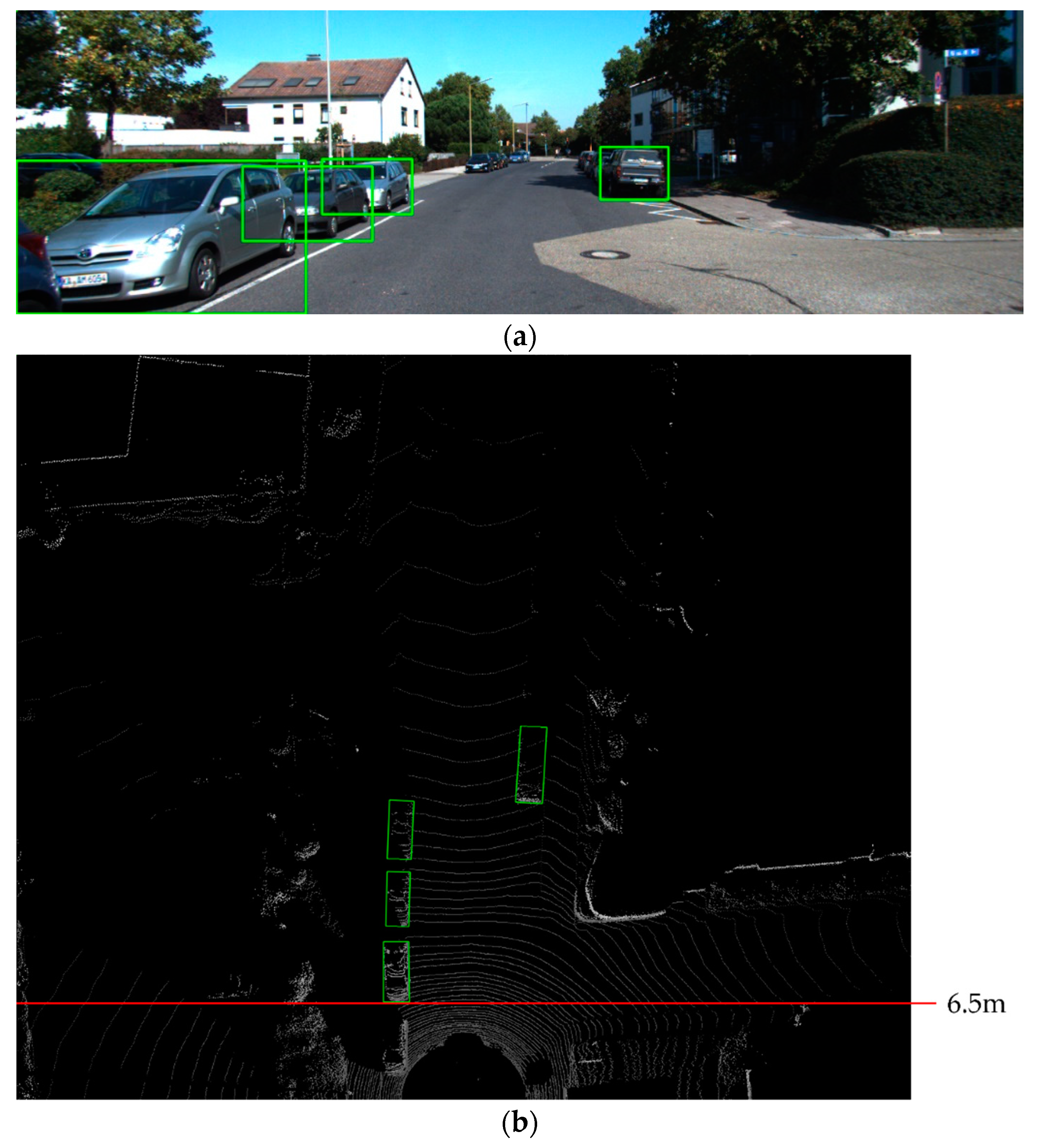
4.1.2. Data Preparation

To train and evaluate the depth outputs, a single representative depth of the ground truth is required. As the 3D object detection dataset provides 3D bounding boxes, we have to convert them into depths. The most important piece of depth information is the closest depth to an object, as we aim to aid risk assessment for self-driving vehicles. The closest depth is extracted by taking the minimum depth among the vertices of a bounding box, as shown in Equation (7).

$$D=\underset{i}{\min }{z}_i$$

(7)

where, $z_i$ is the depth coordinate of the i-th vertex of a 3D bounding box. The example data are shown in Figure 2. The bounding boxes are drawn in the camera image, and the depth of the closest vehicle is depicted in the bird’s-eye view image.

4.1.3. Evaluation Metrics

We define the error rate of the depth per object with Equation (8).

$$E=\frac{\left|D_{gt}-D_{pred}\right|}{D_{grtr}}$$

(8)

Since the error can be calculated with a pair of ground truth and predicted depths, we only calculate the error with true-positive object pairs. The total error will be calculated as the sum of the error rate divided by the number of ground truth objects.

4.1.4. Settings in Detail

We train our YOLO MDE model with two different classes, i.e., car and pedestrian cases, to compare the performance with other models. The input images are scaled to 384 $\times$ 1248 for the large model and 256 $\times$ 832 for the small model. For the anchor box parameter, we use k-means clustering and get the following nine pairs of base anchors: (30, 37), (94, 38), (46, 78), (69, 132), (180, 85), (98, 202), (173, 214), (159, 299), and (191, 396).

The network is optimized by Adam, and we set the learning rate to 0.0001; this is decreased by 0.1 times every 20 epochs until the final 60-th epoch is carried out. We take a mini-batch size of four on a single Nvidia GeForce RTX 3090 (24 GB).

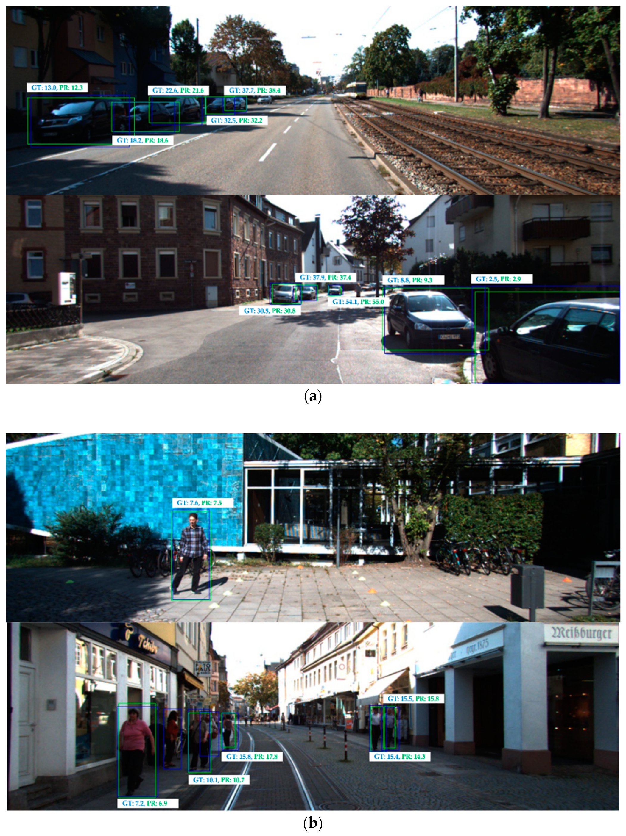
4.2. Training Result and Performance

4.2.1. Performance Comparison

Our model is evaluated by the validation split of the KITTI 3D object detection benchmark and compared with existing studies, i.e., D4LCN [14] and GM3D [17]. Both studies predict 3D bounding boxes from monocular images. Since our model predicts only a single depth per object, only the closest depth of the predicted 3D box is evaluated for the existing models. The depth is extracted in the same manner as the data preparation method described in the previous section. The results are summarized in

Table 1. Performance comparison between 3D object detection models.

Models	AP (Car)	AP (Pedestrian)	Input Size	Depth Error Rate	FPS 1
D4LCN [14]	67.42%	47.56%	288 × 1280	4.07%	5
GM3D [17]	59.61%		512 × 1760	2.77%	20
Yolo MDE	56.73%	55.20%	256 × 832	4.23%	34
Yolo MDE Large	71.68%	62.12%	384 × 1248	3.71%	25

¹ To measure FPS, a single GPU of Tesla V100 was used.

.

The score threshold for the non-maximum suppression (NMS) varies when computing the average precision (AP), but it should be fixed to evaluate the depth error rate. We used the default values in the GitHub source code for the existing models. In our model, 0.85 is selected for the score threshold.

We limited the maximum depth value up to 60 m for calculating the error rate. D4LCN [14] detected cars and pedestrians and had a 4.07% depth error rate with a precision of 74% and a recall of 37%. In [17], the precision and recall increased up to 89% and 42%, respectively, while the depth error rate decreased to 2.77%; however, this model can only detect cars. For our model, we experimented with two types of input resolutions with two classes. The higher input resolution yielded higher accuracy for object detection and depth estimation. Our larger model had a 3.71% depth error, which is comparable to the other models, but showed higher precision and recall values of 96% and 56%, respectively. In addition, our larger model achieved the detection speed of 25 FPS which is five times faster than D4LCN, and 25% faster than GM3D.

The qualitative results are shown in Figure 3. Our model is capable of predicting precise depths for a longer range, as compared to the existing models. The figure shows that the depth errors at more than 40 m are within a few meters.

4.2.2. Ablation Study

To experiment with different network architectures, we tried two different architectures: YOLO v3 [22] and YOLO v4 [19]. YOLO v3 combines the Darknet53 backbone and FPN [34] neck to extract features. We used a 384 $\times$ 1248 size image when using YOLO v3 architecture.

We also tried to use three types of activation functions to decode the model output for depth estimation.

Table 2. Ablation study results.

Network	Activation	AP (Car)	AP (Pedestrian)	Depth Error Rate
Darknet53 + FPN	Exponential	53.94%	48.27%	4.28%
	Reciprocal-Sigmoid	54.07%	41.99%	3.87%
	Log-Sigmoid	68.32%	55.61%	3.35%
CSP-Darknet53 + PAN Large	Exponential	66.54%	59.47%	4.70%
	Reciprocal-Sigmoid	68.83%	61.31%	3.83%
	Log-Sigmoid	71.68%	62.12%	3.71%
CSP-Darknet53 + PAN	Exponential	54.88%	46.10%	4.07%
	Reciprocal-Sigmoid	53.30%	47.16%	3.99%
	Log-Sigmoid	56.72%	55.80%	3.67%

shows the results using various combinations of network architectures and activation functions. The YOLO v3 architecture with log-sigmoid activation function achieved the lowest depth error rate of 3.35%, and the YOLO v4 architecture with log-sigmoid activation function achieved the highest detection performance. The table also shows that the log-sigmoid function always achieved the highest performance regardless of network architecture. In addition, we tried to train the model with common activation functions such as RELU, resulting in a depth error rate of 56% which can be considered as a failure in training depth.

4.2.3. A2D2 Dataset

To generalize our findings, we tried another dataset: A2D2 [35] dataset. Since the A2D2 dataset does not have 2D bounding box labels, we extracted boxes from semantic segmentation labels. The dataset provides 3D bounding box labels, but the 3D labels are not mapped to the extracted 2D boxes. We extracted a single depth per object from LiDAR points within the 2D box instead of using 3D boxes as described in Section 4.1.2.

For training, we tried three different activation functions in Equations (1)–(3). We trained to detect only cars and the results are shown in

Table 3. Training YOLO MDE with A2D2 dataset.

Network	Activation	AP (Car)	Depth Error Rate
CSP-Darknet53 + PAN	Exponential	76.94%	10.14%
	Reciprocal-Sigmoid	77.75%	10.41%
	Log-Sigmoid	77.94%	11.12%

. Since the depth label extracted LiDAR points are not manually corrected, it may contain errors. The result shows a higher depth error rate than that of the KITTI dataset. It proves that extracting depth from the 3D bounding box can help train the depth prediction.

5. Conclusions

In an autonomous driving situation, it is important to detect obstacles and estimate geometric information with low computational cost. We proposed a 2D object detection model with a single depth estimation using a monocular image to simplify both network architecture and prediction parameters.

We compared our model with the latest studies on 3D object detection models [14,17] using the KITTI dataset and monocular camera imaging. Our model achieved an AP of 71.68% for cars which is about 4% and 12% higher than that of D4LCN [14] and GM3D [17], respectively. In addition, our model resulted in an AP of 62.12% for pedestrians which is nearly 14% higher than that of [14]. In terms of comparing detection speed, our model can process 25 frames per second with a single GPU of Tesla V100, and it is five times faster than [14], and 25% faster than [17] with the same computational resources. For the depth estimation, our model achieved 3.71% of the depth error rate, which is 0.36% lower than that of [14], while 0.94% higher than that of [17]. Thus, our model can detect objects with higher speed and accuracy while maintaining a depth error rate compared to the latest 3D object detection model.

As shown in the experiment, the proposed method can be applied to all the other object detection models. We only tried using two different network architectures: YOLO v3 and YOLO v4. Since we focused on higher detection speed, we used only one-stage detectors for the experiment. To improve the detection performance, adapting different object detection architecture such as EfficientDet [25] is expected in future works.

For further research, our model may be applied to object tracking tasks. Object tracking is accomplished by identifying objects in a video and finding their trajectories. Since our model can predict the closest depth per object, the depths and the center points of the bounding box can be transformed into 3D points. A 3D point for an object does not change significantly in a video, so identifying objects can be accomplished by tracking 3D points per object.

References

1. Liu, Z.; Zhao, X.; Huang, T.; Hu, R.; Zhou, Y.; Bai, X. Tanet: Robust 3D object detection from point clouds with triple attention. In Proceedings of the AAAI Conference on Artificial Intelligence, New York, NY, USA, 7–12 February 2020; pp. 11677–11684. [Google Scholar]
2. Zhou, Y.; Tuzel, O. Voxelnet: End-to-end learning for point cloud based 3D object detection. In Proceedings of the IEEE Conference on Computer Vision and Pattern Recognition, Salt Lake City, UT, USA, 18–23 June 2018; pp. 4490–4499. [Google Scholar]
3. Yan, Y.; Mao, Y.; Li, B. Second: Sparsely embedded convolutional detection. Sensors 2018, 18, 3337. [Google Scholar] [CrossRef] [PubMed] [Green Version]
4. Shi, S.; Guo, C.; Jiang, L.; Wang, Z.; Shi, J.; Wang, X.; Li, H. Pv-rcnn: Point-voxel feature set abstraction for 3D object detection. In Proceedings of the IEEE/CVF Conference on Computer Vision and Pattern Recognition, Seattle, WA, USA, 13–19 June 2020; pp. 10529–10538. [Google Scholar]
5. Chen, X.; Ma, H.; Wan, J.; Li, B.; Xia, T. Multi-View 3D Object Detection Network for Autonomous Driving. In Proceedings of the IEEE conference on Computer Vision and Pattern Recognition, Honolulu, HI, USA, 21–26 June 2017; pp. 1907–1915. [Google Scholar]
6. Li, B.; Zhang, T.; Xia, T. Vehicle Detection from 3D Lidar Using Fully Convolutional Network. 2016. Available online: https://arxiv.org/abs/1608.07916 (accessed on 24 November 2021).
7. Yang, B.; Luo, W.; Urtasun, R. PIXOR: Real-Time 3D Object Detection from Point Clouds. In Proceedings of the IEEE Conference on Computer Vision and Pattern Recognition, Salt Lake City, UT, USA, 18–23 June 2018; pp. 7652–7660. [Google Scholar]
8. Liang, M.; Yang, B.; Wang, S.; Urtasun, R. Deep Continuous Fusion for Multi-Sensor 3D Object Detection. In Proceedings of the European Conference on Computer Vision (ECCV), Munich, Germany, 8–14 September 2018; pp. 641–656. [Google Scholar]
9. Ku, J.; Mozifian, M.; Lee, J.; Harakeh, A.; Waslander, S. Joint 3D Proposal Generation and Object Detection from View Aggregation. In Proceedings of the 2018 IEEE/RSJ International Conference on Intelligent Robots and Systems (IROS), Madrid, Spain, 1–5 October 2018; pp. 1–8. [Google Scholar]
10. Ma, X.; Wang, Z.; Li, H.; Zhang, P.; Ouyang, W.; Fan, X. Accurate Monocular 3D Object Detection via Color-Embedded 3D Reconstruction for Autonomous Driving. In Proceedings of the IEEE/CVF International Conference on Computer Vision, Long Beach, CA, USA, 15–20 June 2019; pp. 6851–6860. [Google Scholar]
11. Chen, X.; Kundu, K.; Zhang, Z.; Ma, H.; Fidler, S.; Urtasun, R. Monocular 3D Object Detection for Autonomous Driving. In Proceedings of the IEEE Conference on Computer Vision and Pattern Recognition, Las Vegas, NV, USA, 27–30 June 2016; pp. 2147–2156. [Google Scholar]
12. Brazil, G.; Liu, X. M3D-RPN: Monocular 3D Region Proposal Network for Object Detection. In Proceedings of the IEEE/CVF International Conference on Computer Vision, Long Beach, CA, USA, 15–20 June 2019; pp. 9287–9296. [Google Scholar]
13. Mousavian, A.; Anguelov, D.; Flynn, J.; Košecká, J. 3D Bounding Box Estimation Using Deep Learning and Geometry. In Proceedings of the IEEE Conference on Computer Vision and Pattern Recognition, Honolulu, HI, USA, 21–26 July 2017; pp. 7074–7082. [Google Scholar]
14. Ding, M.; Huo, Y.; Yi, H.; Wang, Z.; Shi, J.; Lu, Z.; Luo, P. Learning Depth-Guided Convolutions for Monocular 3D Object Detection. In Proceedings of the IEEE/CVF Conference on Computer Vision and Pattern Recognition, Seattle, WA, USA, 13–19 June 2020; pp. 1000–1001. [Google Scholar]
15. Li, P.; Chen, X.; Shen, S. Stereo R-CNN Based 3D Object Detection for Autonomous Driving. In Proceedings of the IEEE/CVF Conference on Computer Vision and Pattern Recognition, Long Beach, CA, USA, 15–20 June 2019; pp. 7644–7652. [Google Scholar]
16. Qin, Z.; Wang, J.; Lu, Y. Triangulation Learning Network: From Monocular to Stereo 3D Object Detection. In Proceedings of the IEEE/CVF Conference on Computer Vision and Pattern Recognition, Long Beach, CA, USA, 15–20 June 2019; pp. 7615–7623. [Google Scholar]
17. Liu, Y.; Yixuan, Y.; Liu, M. Ground-Aware Monocular 3D Object Detection for Autonomous Driving. Robot. Autom. Lett. 2021, 6, 919–926. [Google Scholar] [CrossRef]
18. Masoumian, A.; Marei, D.G.; Abdulwahab, S.; Cristiano, J.; Puig, D.; Rashwan, H.A. Absolute distance prediction based on deep learning object detection and monocular depth estimation models. In Proceedings of the 23rd International Conference of the Catalan Association for Artificial Intelligence, Artificial Intelligence Research and Development, Lleida, Spain, 20–22 October 2021; pp. 325–334. [Google Scholar]
19. Bochokvskiy, A.; Wang, C.-Y.; Liao, H.-Y.M. YOLOv4: Optimal Speed and Accuracy of Object Detection. 2020. Available online: https://arxiv.org/abs/2004.10934 (accessed on 23 April 2020).
20. Geiger, A.; Lenz, P.; Stiller, C.; Urtasun, R. Vision Meets Robotics: The KITTI Dataset. Int. J. Robot. Res. 2013, 32, 1231–1237. [Google Scholar] [CrossRef] [Green Version]
21. He, K.; Zhang, X.; Ren, S.; Sun, J. Deep Residual Learning for Image Recognition. In Proceedings of the IEEE Conference on Computer Vision and Pattern Recognition, Las Vegas, NV, USA, 27–30 June 2016; pp. 770–778. [Google Scholar]
22. Redmon, J.; Farhadi, A. YOLOv3: An Incremental Improvement. 2018. Available online: https://arxiv.org/abs/1804.02767 (accessed on 8 April 2018).
23. Law, H.; Deng, J. CornerNet: Detecting Objects as Paired Keypoints. In Proceedings of the European Conference on Computer Vision (ECCV), Munich, Germany, 8–14 September 2018; pp. 734–750. [Google Scholar]
24. Duan, K.; Bai, S.; Xie, L.; Qi, H.; Huang, Q.; Tian, Q. CenterNet: Keypoint Triplets for Object Detection. In Proceedings of the IEEE/CVF International Conference on Computer Vision, Long Beach, CA, USA, 15–20 June 2019; pp. 6569–6578. [Google Scholar]
25. Tan, M.; Pang, R.; Le, Q. EfficientDet: Scalable and Efficient Object Detection. In Proceedings of the IEEE/CVF Conference on Computer Vision and Pattern Recognition, Seattle, WA, USA, 13–19 June 2020; pp. 10781–10790. [Google Scholar]
26. Girshick, R.; Donahue, J.; Darrell, T.; Malik, J. Rich Feature Hierarchies for Accurate Object Detection and Semantic Segmentation. In Proceedings of the IEEE Conference on Computer Vision and Pattern Recognition, Columbus, OH, USA, 23–28 June 2014; pp. 580–587. [Google Scholar]
27. Purkait, P.; Zhao, C.; Zach, C. SPP-Net: Deep Absolute Pose Regression with Synthetic Views. 2017. Available online: https://arxiv.org/abs/1712.03452 (accessed on 9 December 2017).
28. Girshick, R. Fast R-CNN. In Proceedings of the IEEE International Conference on Computer Vision, Boston, MA, USA, 7–12 June 2015; pp. 1440–1448. [Google Scholar]
29. Ren, S.; He, K.; Girshick, R.; Sun, J. Faster R-CNN: Towards Real-Time Object Detection with Region Proposal Networks. IEEE Trans. Pattern Anal. Mach. Intell. 2017, 39, 1137–1149. [Google Scholar] [CrossRef] [PubMed] [Green Version]
30. Wang, C.-Y.; Liao, H.-Y.M.; Wu, Y.-H.; Chen, P.-Y.; Hsieh, J.-W.; Yeh, I.-H. CSPNet: A New Backbone That Can Enhance Learning Capability of CNN. In Proceedings of the IEEE/CVF Conference on Computer Vision and Pattern Recognition Workshops, Seattle, WA, USA, 14–19 June 2020; pp. 390–391. [Google Scholar]
31. Liu, S.; Qi, L.; Qin, H.; Shi, J.; Jia, J. Path Aggregation Network for Instance Segmentation. In Proceedings of the IEEE Conference on Computer Vision and Pattern Recognition, Salt Lake City, UT, USA, 18–23 June 2018; pp. 8759–8768. [Google Scholar]
32. Zheng, Z.; Wang, P.; Liu, W.; Li, J.; Ye, R.; Ren, D. Distance-IoU Loss: Faster and Better Learning for Bounding Box Regression. In Proceedings of the AAAI Conference on Artificial Intelligence, New York, NY, USA, 7–12 February 2020; pp. 12993–13000. [Google Scholar]
33. Huber, P. Robust Estimation of a Location Parameter. In Breakthroughs in Statistics; Springer: New York, NY, USA, 1992; pp. 492–518. [Google Scholar]
34. Lin, T.-Y.; Dollár, P.; Girshick, R.; He, K.; Hariharan, B.; Belongie, S. Feature Pyramid Networks for Object Detection. In Proceedings of the IEEE Conference on Computer Vision and Pattern Recognition, Honolulu, HI, USA, 21–16 July 2017; pp. 2117–2125. [Google Scholar]
35. Geyer, J.; Kassahun, Y.; Mahmudi, M.; Ricou, X.; Durgesh, R.; Chung, A.S.; Hauswald, L.; Pham, V.H.; Mühlegg, M.; Dorn, S.; et al. A2D2: Audi Autonomous Driving Dataset. 2020. Available online: https://arxiv.org/abs/2004.06320 (accessed on 14 April 2020).
Figure 1. The network overview of our detection model. We add a single depth channel to the output of YOLO v4 to predict depth information for each object. The depth channel is trained with single ground truth depth information. The ground truth depth will be discussed in Section 3.2.1.
Electronics 11 00076 g001
Figure 2. (a) Three-dimensional boxes projected onto a 2D image and (b) 3D boxes projected onto a bird’s-eye view image with the depth calculation based on pixels.
Electronics 11 00076 g002
Figure 3. The prediction result of (a) Cars and (b) Pedestrians. Blue bounding boxes represent the ground truth, and green bounding boxes represent the detection results.
Electronics 11 00076 g003