Article

Global Sensitivity Analysis of Economic Model Predictive Longitudinal Motion Control of a Battery Electric Vehicle

1
Department of Electrical Engineering, University of Applied Sciences Trier, Schneidershof, 54293 Trier, Germany
2
Interdisciplinary Centre for Security, Reliability and Trust, University of Luxembourg, 29 Av. J.F. Kennedy, 1855 Luxembourg, Luxembourg
*
Author to whom correspondence should be addressed.
Electronics 2022, 11(10), 1574; https://doi.org/10.3390/electronics11101574
Submission received: 13 April 2022 / Revised: 11 May 2022 / Accepted: 11 May 2022 / Published: 14 May 2022

Abstract

:
Global warming forces the automotive industry to reduce real driving emissions and thus, its CO2 footprint. Besides maximizing the individual efficiency of powertrain components, there is also energy-saving potential in the choice of driving strategy. Many research works have noted the potential of model predictive control (MPC) methods to reduce energy consumption. However, this results in a complex control system with many parameters that affect the energy efficiency. Thus, an important question remains: how do these partially uncertain (system or controller) parameters influence the energy efficiency? In this article, a global variance-based sensitivity analysis method is used to answer this question. Therefore, a detailed powertrain model controlled by a longitudinal nonlinear MPC (NMPC) is developed and parameterized. Afterwards, a qualitative Morris screening is performed on this model, in order to reduce the parameter set. Subsequently, the remaining parameters are quantified using Generalized Sobol Indices, in order to take the time dependence of physical processes into account. This analysis reveals that the variations in vehicle mass, battery temperature, rolling resistance and auxiliary consumers have the greatest influence on the energy consumption. In contrast, the parameters of the NMPC only account for a maximum of 5% of the output variance.

1. Introduction

Considering global warming and the targeted reduction of greenhouse gas emissions by governments, the transformation to electromobility plays an important role in reaching climate goals. Great potential to reduce these emissions lies in replacing conventional vehicle propulsion systems with electric propulsion systems, as outlined in [1]. It is shown that the change to electric vehicles avoid local emmissions, which improves the air quality, especially in larger cities. Furthermore, the dependence on oil imports is reduced. Nevertheless, there are many other aspects that can reduce the energy consumption of vehicles, including environmental conditions, such as the weather or road surface conditions, the driving style of the driver and the vehicle itself [2]. Especially for battery electric vehicles (BEVs) with long recharge times and lower ranges than internal combustion engines saving energy during operation plays a crucial role. Thus, the development of energy-efficient driving strategies to reduce fuel consumption have gained significant industrial interest [3]. As a vehicle can only be optimized during the development process and usually not influenced during operations, the development of eco-driving strategies to optimize the operation of vehicles has received great attention. Eco-driving generally describes the reduction of fuel consumption by operating the vehicle along its energy-optimal velocity trajectory. It can be processed by a human driver using learned patterns to achieve low energy consumption; for example, through smooth acceleration or deceleration and maintaining a constant speed. Furthermore, eco-driving is capable of reducing traffic fatalities and can reduce the risk of traffic accidents [3]. However, without exact knowledge of the energy-optimal operating points of the vehicle and the upcoming driving situation, a human driver can only reach a sub-optimal driving strategy.
The increasing availability of environmental data and the processing power of modern vehicle platforms has enabled the development of advanced eco-driving algorithms, which consider environmental information and the actual vehicle state to optimize the driving strategy. To address this multi-objective target, most approaches focus on model predictive controllers (MPC) as a promising optimization approach for real-time optimal control. MPCs are often designed as a linear quadratic problem to achieve real-time capability [4,5,6,7]. This simpler—but computationally effective—design usually leads to simplifications of the system model of the MPC. In [4,5], the energy consumption of the underling powertrain components was approximated using a convex lookup table. Combined spatial–temporal modeling to ensure a linear optimization problem has been proposed in [7]. Furthermore, explicit solutions for the driving strategy (see, e.g., [6]) involve solving the optimization problem offline and storing the results in a lookup table.
To overcome these approximations, nonlinear MPC (NMPC) approaches [8,9,10,11,12,13,14] have been outlined in the literature. These approaches ensure more accurate modeling of the control problem. To ensure real-time capability, the nonlinear approaches are often solved using dynamic programming [10,11] or calculated online using an efficient NMPC solver [8,9,12,14], such as C/GMRES. Furthermore, stochastic approaches, mainly for modeling the non-deterministic surrounding traffic, have also been presented in the literature [15,16,17,18,19].
The application of MPC based longitudinal motion control has been applied to internal combustion engine vehicles [6,8,9], hybrid electric vehicles [13,14], and pure electric vehicles [4,5,7,10,12,15,16,17].
All of the approaches mentioned above are complex closed-loop control systems with a large number of system and controller parameters, which all influence the system behavior. Therefore, the important question remains: how can the influence of parameters on the energy consumption and the driving behavior be quantified, which normally cannot be done analytically in such complex systems? To answer this question, qualitative- and quantitative-based sensitivity analysis methods to analyze and quantify parameter dependencies have been proposed in the literature. The most popular and promising methods are qualitative Morris parameter screening [20] and the variance-based sensitivity analysis, first introduced by Sobol [21]. In particular, in the context of analyzing the energy efficiency of BEVs several studies exist which highlight the potential of statistical investigation. In the work of [22], parameter dependencies on the energy efficiency were investigated during a field test with six buses on three different routes using regression coefficients. Furthermore, [23] have outlined a surrogate model to predict the energy consumption of electrical buses and performed a sensitivity analysis to determine parameter dependencies in their prediction using Sobol indices. A sensitivity analysis of a BEV using Sobol indices has been outlined in [24], which was performed on previously recorded velocity profiles for typical urban and rural use-cases in the Vienna area. Nevertheless, this work is based on a simple longitudinal motion model only considering efficiency rates in the electric drivetrain. More detailed sensitivity analyses on specific drivetrain components and not at the vehicle level have been conducted in [25,26,27,28]. In [25], a qualitative Morris screening was performed to analyze a basic equivalent circuit model of a battery system. A Morris screening-based investigation considering the reaction kinematic models of a battery has been detailed in [26]. Parameter dependencies on the torque accuracy of an electric drive system using Sobol indices have been outlined in [27]. Furthermore, a good review regarding sensitivity analysis for electrical drives can be found in [28]. Beside the aforementioned applications [29] have underlined the increasing demand for systematic analyses of complex mathematical models across different disciplines.
However, the aforementioned publications at vehicle level have not included detailed powertrain models, whereas the component-level evaluations did not take dependencies at the system level into account. Furthermore, the outlined investigations were carried out using pre-recorded velocity profiles at vehicle level or specific working points or load profiles at component level. Therefore, this article outlines a novel approach for analyzing a closed-loop economic NMPC-based eco-driving system of a BEV using Morris screening and variance-based sensitivity analysis. Furthermore, in contrast to the known literature, the drivetrain components considered in this investigation are modeled in great detail, and are optimized with respect to accuracy and calculation time, in order to obtain reliable sensitivity results. Furthermore, the time dependence of physical processes is considered in the sensitivity analysis, through the use of Generalized Sobol indices [30].
The remainder of this article is organized as follows: Section 2 outlines the theory of the used sensitivity analysis methods of Morris Screening, Sobol indices and Generalized Sobol Indices. In Section 3, the developed and used simulation models are presented. Section 4 presents the economic NMPC used in this investigation. In Section 5, the sensitivity analysis setup is defined and in Section 6, the results of the sensitivity analysis are discussed. Section 7 concludes the presented findings of this article.

2. Sensitivity Analysis

The process of a variance-based sensitivity analysis is shown in Figure 1. Based on the uncertainties of different model parameters X = [ X 1 , X 2 ,   , X k ] , described by their probability density functions, a classical uncertainty analysis is performed. This is usually done by carrying out a Monte-Carlo simulation, where the result is a distribution of the model output Y. However, in an uncertainty analysis, no conclusions can be drawn about the cause of the variance. The sensitivity analysis closes this gap and enables a quantification of the influencing factors. This makes it possible to specifically influence the relevant parameters, thus reducing the output variance. As the quantitative variance-based sensitivity analysis (outlined in Section 2.2) is a computationally expensive task, qualitative Morris screening [20] is used in advance, in order to identify parameters that have nearly no effect on the output of interest. Therefore, the computational burden of the quantitative analysis is reduced by neglecting non-influential parameters from the simulation study.

2.1. Morris Screening

Morris Screening, according to [20], offers an efficient method for the qualitative estimation of the influences of parameters on a model output. The main idea is based on the elementary effect
E E i = f ( x 1 , x 2 , , x i 1 , x i + Δ , x i + 1 , , x k ) f ( x ) Δ
for a given model y = f ( x ) , with y as the model output and x = [ x 1 , x 2 , , x k ] as the parameter input vector. Due to the addition of the small variation Δ to the ith parameter and in the denominator, the elementary effect can be understood as a partial difference quotient. This OAT-design needs to be calculated k + 1 times to obtain one elementary effect for each parameter. In [20], a novel scheme for defining the trajectory through this input parameter space was proposed. However, using only one elementary effect calculation for each parameter does not provide a satisfactory covering of the input parameter space. Therefore, the calculation of elementary effects is done for r different input trajectories with varying starting points. This results in N m = r ( k + 1 ) needed simulation runs, where [31,32] have shown that r = 10 is a typical value for producing valuable results.
As sensitivity measures, the mean μ i , the mean of the absolute values μ i * and the standard deviation σ i of the elementary effects are considered. The measures
μ i = 1 r j = 1 r E E i j
and
σ i = 1 r 1 j = 1 r ( E E i j μ i ) 2
were first presented in [20]. Here, μ i assesses the overall influence of the ith parameter on the output, whereas σ i is an effective measure to estimate nonlinear or interaction effects in the model. However, using the proposed measure μ i has the disadvantage that type II errors can occur, which may result in failing to identify factors with considerable influence on the output. The measure
μ i * = 1 r j = 1 r | E E i j | ,
first introduced by [33], avoids type II errors by using the absolute values of the elementary effects.
The measures presented above are used to rank the importance of the parameters. Small values of μ i * in relation to other parameters indicate a small influence on the output and so, such parameters can be neglected in the quantitative sensitivity setup. In contrast, large values in comparison to the other parameters express a strong influence and the related parameters must be considered in the quantitative sensitivity setup.

2.2. Variance-Based Sensitivity Analysis

As outlined in [21], the idea of a variance-based sensitivity analysis is the decomposition of a model y = f ( x ) with x = [ x 1 , x 2 , , x k ] in a sum of 2 k terms using a High-Dimensional Model Representation (HDMR) in the form
y = f ( x ) = f 0 + i = 1 k f i ( x i ) + i = 1 k i < j k f i j ( x i , x j ) + + f 12 k ( x 1 , x 2 , , x k ) ,
where f 0 describes a constant term without any dependencies on the input vector, whereas the k terms f i ( x i ) describe first-order functions with dependencies on only one input parameter x i . This scheme can be continued up to n k = n ! k ! ( n k ) ! terms, representing nth order functions with dependencies on n input parameters. Assuming independence of the parameters and orthogonality of the terms in (5), the variance is given by
V ( Y ) = ( f ( x ) f 0 ) 2 m = 1 k p m ( X m ) d x = i = 1 k V i + i = 1 k i < j k V i j + + V 12 k ,
with p m being the probability density function of the corresponding input parameter X m . The variances of the corresponding terms are defined by
V i = V ( f i ( x i ) ) = f i 2 ( x i ) p i ( X i ) d x i
V i j = V ( f i j ( x i , x j ) ) = f i j 2 ( x i , x j ) p i ( X i ) p j ( X j ) d x i d x j
V 12 k = V ( f 12 k ( x 1 , x 2 , , x k ) ) = f 12 k 2 ( x 1 , x 2 , , x k ) m = 1 k p m ( X m ) d x .
Normalizing (6) by V ( Y ) leads to
1 = i = 1 k S i + i = 1 k i < j k S i j + + S 12 k ,
which serves as a decomposition of the source of variance. The terms containing S i are referred to as first-order effects. They quantify the influence of the parameter x i without interactions to other parameters to the output y. S i j denotes the second-order effects, which indicate the interaction between two parameters x i , x j . This decomposition scheme can be continued up to the kth-order effects.
Another useful measure, especially for describing all nonlinear interaction effects, is the total effect
S T i = S i + j = 1 j i k S i j + + S 12 k ,
which sums up all effects of one parameter, including all higher-order effects.
As outlined in [34], the first-order indices can be calculated using the relation of the conditional expectation value V X i ( E X i ( Y X i ) ) and the overall variance V ( Y ) , described by
S i = V X i ( E X i ( Y X i ) ) V ( Y ) ,
where X i denotes the vector of all parameters except X i . The expectation operator E X i ( · ) calculates the average over X i , whereas X i is fixed and the outer variance V X i ( · ) is taken over all realizations of X i .
The total effect is calculated using [34,35]
S T i = E X i ( V X i ( Y X i ) ) V ( Y ) = 1 V X i ( E X i ( Y X i ) ) V ( Y ) .
An obvious explanation is to consider that V X i ( E X i ( Y X i ) ) is the first-order effect of X i . Consequently, V ( Y ) V X i ( E X i ( Y X i ) ) must include all terms in the variance decomposition of (6) which include X i .
The decomposition presented in (5) leads to 2 k 1 possible sensitivity measures. Due to the large number of indices, it is impractical to analyze all of them. Nevertheless, the first-order and the total effects approximate the system behavior satisfactorily, such that higher-order effects can usually be neglected. In addition, estimation of the conditional expectation values using Monte-Carlo simulations is computationally expensive and therefore, only the first-order and total effects are considered.
The indices can be interpreted as the expected reduction of variance. The numerator of the first order effects V X i ( E X i ( Y X i ) ) describes the reduction of variance in the output Y if X i were fixed at some defined value. Furthermore, the numerator of the total effect E X i ( V X i ( Y X i ) ) is the amount of variance that would remain if all factors but X i were fixed. The ordering of the sensitivity measures quantify their contribution to the overall variance. In other words, small sensitivity measures have only a small influence on the variance of the output, whereas large measures have a big influence on the output. Moreover, the sensitivity measures have some general properties which are useful to analyze the structure of the model:
  • Due to (10), the condition i = 1 k S i 1 holds.
  • Due to (11), the condition i = 1 k S T i 1 holds.
  • If i = 1 k S i = 1 , the model is additive.
  • If 1 i = 1 k S i 0 , the model has nonlinear behavior or interacting parameters.
  • If S T i S i , no interactions exists. This also implies the additivity of the model.
  • If S T i 0 , the parameter has no influence on the output.

2.3. Time and State Dependency of Technical Processes

The main drawback of the HDMR described in (5) is that it neglects state and time dependencies, regarding the physical systems. Thus, the underlying model needs to be expanded to
y ( t ) = f ( x , x 0 , t , u ( t ) ) ,
where x 0 denotes the initial system state. Furthermore, the system consists of a control vector u = [ u 1 , u 2 , , u c ] , with c being the number of control inputs. The proposed extension by x 0 , t and u ( t ) leads also to state- and time-dependent sensitivity indices. As already outlined in [27], the dependency of x 0 and u ( t ) can be ensured by covering all the relevant operating points of the physical system. In this article, this is ensured by defining representative drive cycles, as outlined in Section 3.4. Thus, (14) can be simplified to
y ( t ) = f ( x , t )
and can also be written as a second-order ANOVA-like decomposition
f ( x , t ) = f U ( x U , t ) + f U ( x U , t ) + f U , U ( x , t ) ,
with the complete index set X = { 1 , , k } , the subset U = { i 1 , i 2 , , i s } X and the complementary subset U = { j 1 , j 2 , , j s } = X\U. The corresponding parameter vectors are x U = [ x i 1 , x i 2 , , x i s ] and x U = [ x j 1 , x j 2 , , x j s ] . The variance of this decomposition is defined as
V ( f , t ) = V U ( f , t ) + V U ( f , t ) + V U , U ( f , t ) ,
where V U = V i holds if the subset U contains only the ith parameter. In this case (17) is equal to (6). In the following, the subset containing only the ith parameter is denoted by U i .
The Sobol indices are usually calculated as point-in-time indices. For the scalar case with V U i = V i , the sensitivity indices can be expressed as follows
S i ( f , t ) = V U i ( f , t ) V ( f , t )
S T i ( f , t ) = V U i ( f , t ) + V U i , U ( f , t ) V ( f , t )
for each t [ 0 , T ] . There are several problems when using only these point-in-time estimates [30]:
  • Point-in-time indices ignore all time correlations of the process.
  • The variance of the process varies in time, which skews the relative importance across time.
To solve the above-mentioned issues, [30] introduced the Generalized Sobol Indices, which are based on a covariance operator to take the evolution of the process over time into account. Furthermore, the second issue regarding skewing is solved by this approach. The Generalized Indices are defined as
S i G ( f , T ) = 0 T V U i ( f , t ) d t 0 T V ( f , t ) d t
S T i G ( f , T ) = 0 T ( V U i ( f , t ) + V U i , U ( f , t ) ) d t 0 T V ( f , t ) d t ,
which can be simply computed using the approximation
S i G ( f , T ) m = 1 N w m V U i ( f , t m ) m = 1 N w m V ( f , t m )
S T i G ( f , T ) m = 1 N w m ( V U i ( f , t m ) + V U i , U ( f , t m ) ) m = 1 N w m V ( f , t m )
in a numerical setup with weights { w m } m = 1 N for each node { t m } m = 1 N . The special case of equal weights and uniform time steps has been suggested in [36] for time-dependent processes, which is used throughout this article. The indices are calculated using the estimators described in [34] and convergence of this estimators is ensured as proposed in [27].

3. Simulation Setup

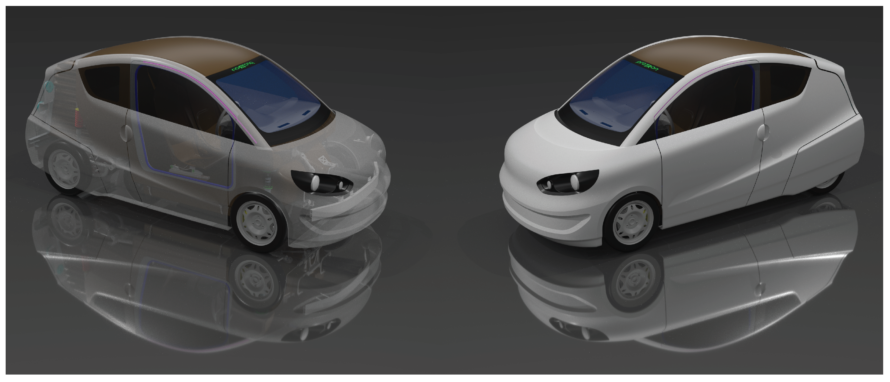
The vehicle serving as the basis for this simulation study is an early-stage prototype for urban and inter-urban use-cases, which is under development at the University of Applied Sciences Trier. A sketch of the proTRon Evolution is provided in Figure 2. The project focuses on sustainable mobility, taking into consideration the complete product life cycle. Due to this fact, the vehicle body is largely made of natural fiber-reinforced plastics, in order to reduce emissions in the manufacturing process. In order to keep energy consumption in driving operations as low as possible, a target weight of 550 kg is planned while, at the same time, complying with the crash safety requirements relevant for approval. Furthermore, all mechanical driving resistances are forced to be as small as possible. This is achieved by using tires with low rolling resistance properties with dimensions 115/80 R 15, in order to reduce the rolling resistance coefficient. Additionally, the aerodynamic drag coefficient and the frontal area of the vehicle were minimized during the development process using CFD simulations, resulting in low aerodynamic resistance. Furthermore, the car uses a novel transmission concept, consisting of a belt drive and a planetary gear with optimized losses within a small installation space. The powertrain of the vehicle consists of a single-wheel drive on the rear axle with EMRAX 188 permanent magnet synchronous drives, which are powered by a series connection of 76 40 Ah Winston WB-LYP40AHA lithium iron phosphate accumulators.
The used simulation setup, including the configuration of the BEV, is outlined in Figure 3. As the underlying component models can highly affect the sensitivity analysis results, they are a crucial part of the simulation setup. Therefore, the models commonly used in the literature are modified with the aim of increasing accuracy and minimizing computation time. In particular, the inverter and electric drive models are optimized, regarding calculation time, to fit into the Monte-Carlo setup of the sensitivity analysis by averaging the losses over one fundamental wave period and neglecting the current dynamics in the electrical drive model. Furthermore, the inverter model is extended to precisely model nonlinear switching losses, especially for low currents. To improve the accuracy of the electrical drive model nonlinear iron losses are taken into account. For the aforementioned reasons and in order to emphasize the nonlinear parameter dependencies of the battery, the battery, inverter and electrical drive component models’, as well as their corresponding parameters are discussed in detail in the following. As the vehicle model is a standard longitudinal motion model, the details are only outlined in Appendix A. The environmental model consists of a route model, including curvature, slope and legal speed limit information. Furthermore, the ambient temperature and air pressure are provided to the simulation environment.

3.1. Battery Model

Modeling the behavior of a modern lithium ion accumulator can be divided according to different complexities and different levels of model knowledge. White-box models based on reaction kinetics [37,38] or physically motivated equivalent circuit modeling [39] provide a detailed basis for understanding the electrochemical processes. However, the complexity of such models also significantly increases the computational cost and parameterization is often only possible with high effort. In contrast, black-box models, such as neural networks [40] and Markov chains [41], may also be used. They are easy to train or parameterize from existing measurement data. However, the major drawback of these modeling is a lack of representation of physical relationships. In order to reduce the complexity without losing a general physical interpretability of the models, simple equivalent circuit models have been established. These range from a simple representation with constant voltage source and internal resistance [42] to electrical RC networks with operating point-dependent parameters [43]. Due to the possible physical interpretability of the parameters, good parameterizability and low computation times, a corresponding equivalent circuit model is used and introduced in the following.

3.1.1. Electrical Model

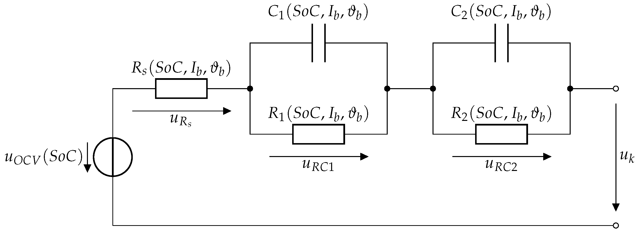
Figure 4 depicts the equivalent circuit diagram of a single battery cell. It consists of a voltage source u O C V , a series resistor R s representing the ohmic losses in the battery cell, and two RC elements describing the cell dynamics. The terminal voltage is calculated using Kirchhoff’s mesh rule, with
u k = n c e l l ( u O C V u R s u R C 1 u R C 2 ) ,
where n c e l l denotes the number of cells connected in series. Using Kirchhoff’s junction rule, the differential equations for the required voltage drops u R C 1 and u R C 2
u ˙ R C 1 = i b u R C 1 R 1 ( S o C , I b , ϑ b ) C 1 ( S o C , I b , ϑ b )
u ˙ R C 2 = i b u R C 2 R 2 ( S o C , I b , ϑ b ) C 2 ( S o C , I b , ϑ b )
can be obtained. Furthermore, the voltage drop on the series resistance is defined by
u R s = R s ( S o C , i b , ϑ b ) i b .
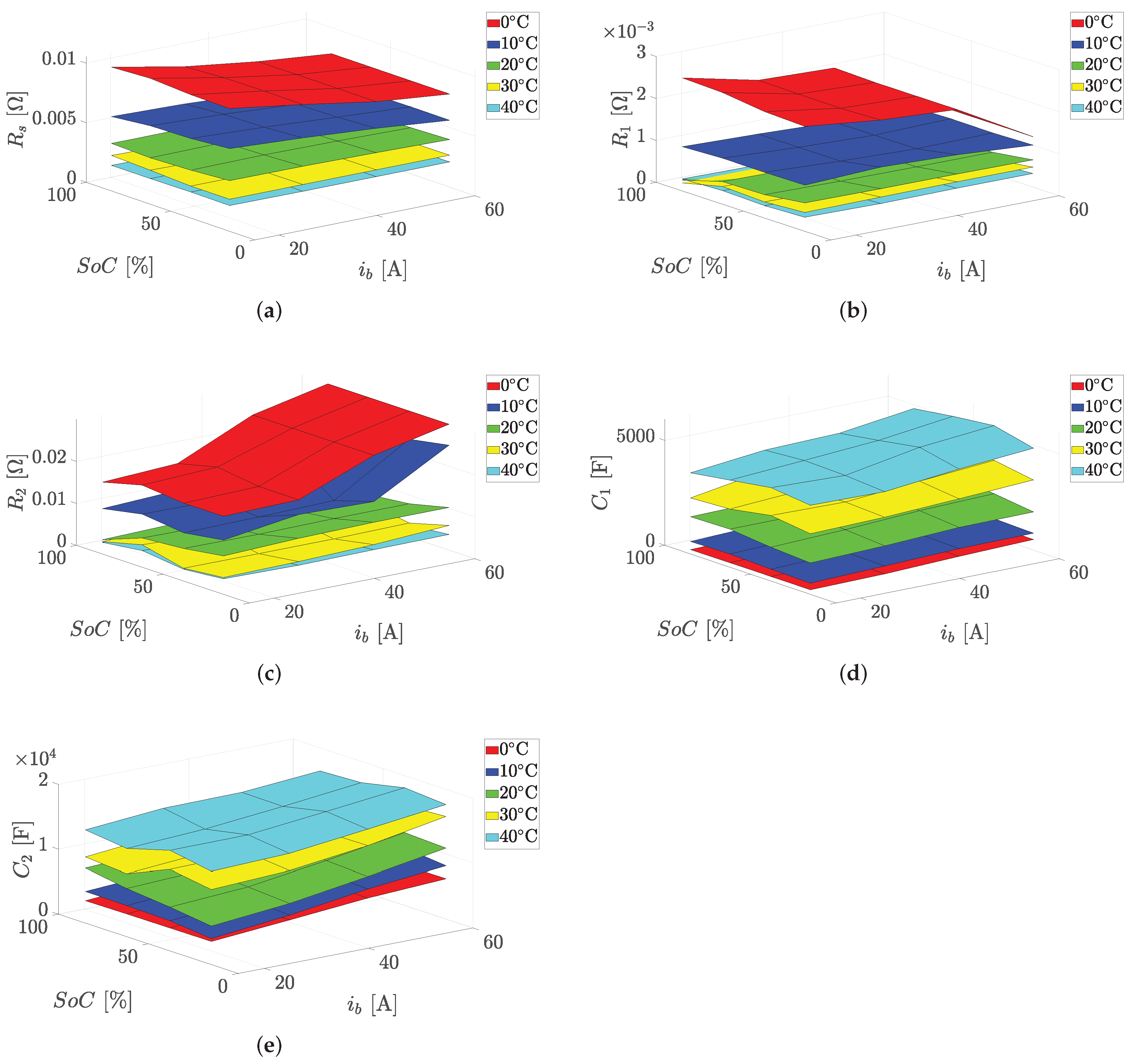
As it can be seen from (25)–(27), as well as from the outlined parameter maps in Figure 5, the parameters R s , R 1 , R 2 , C 1 and C 2 depend on the actual operating point of the battery cell, which is defined by the State of Charge (SoC)
S o C = Q S o C Q b ( ϑ b ) ,
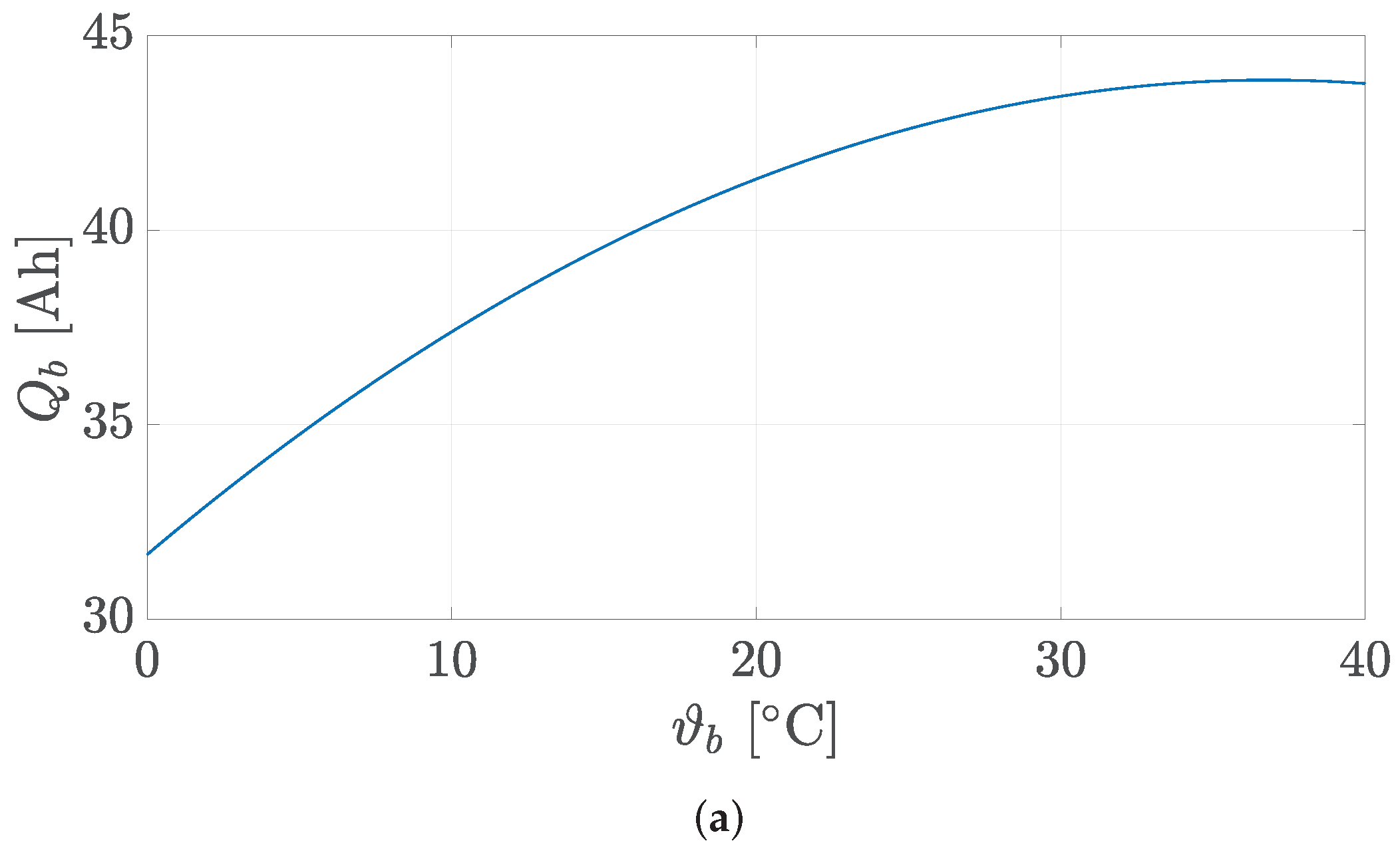
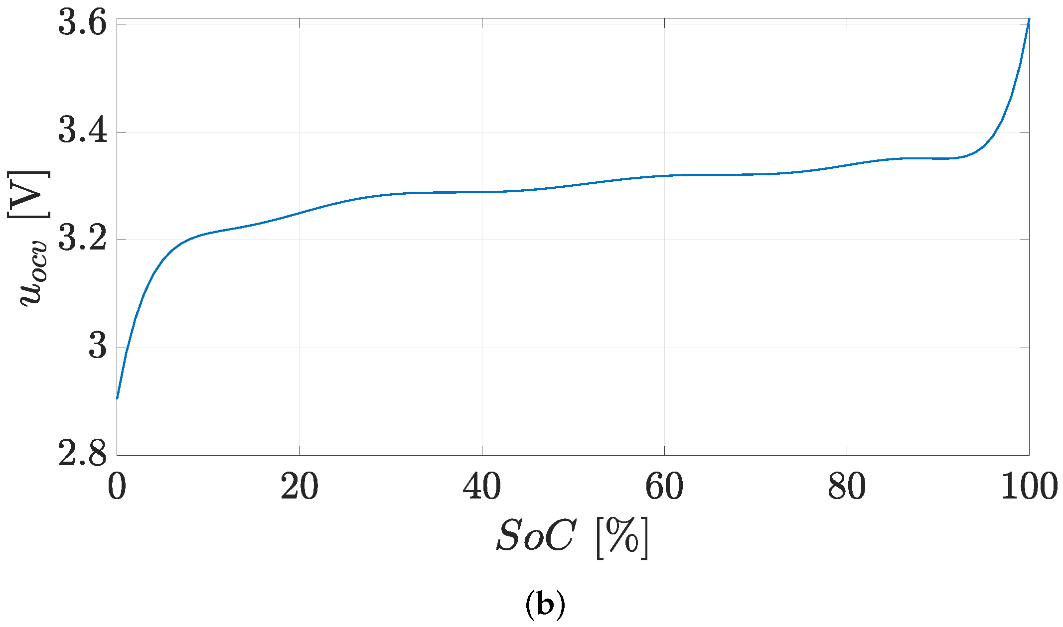
the battery current i b and the battery temperature ϑ b . Q S o C defines the actual stored electrical charge, whereas Q b is the maximum available electrical charge of one cell. Furthermore, the open circuit voltage u O C V depends on the actual SoC and Q b is influenced by ϑ b , as outlined in Figure 6. The aforementioned electrical parameters of the used battery cells were acquired from [44] and are outlined in Figure 5 and Figure 6.

3.1.2. Thermal Model

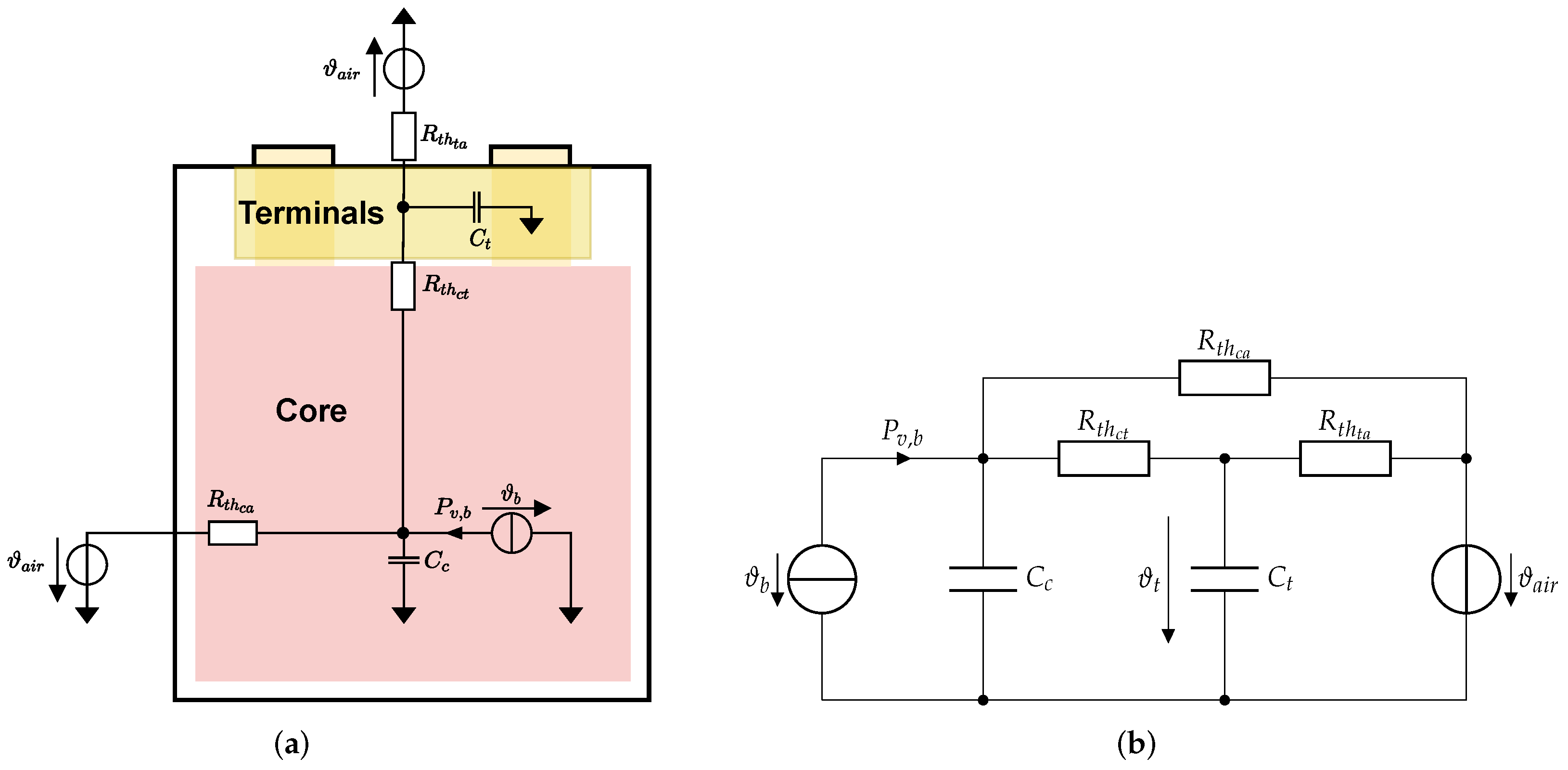
Figure 7 outlines the model used for the thermal behavior of a battery cell. In Figure 7a, the cross-section of one cell is outlined. The red part in this scheme consists of the battery housing and the reactive part of the cell, including the anode, cathode, separator and electrolyte, whereas the yellow part describes the metallic connection of the cell core to the terminals. The corresponding heat capacities are assigned to the two areas of the cell. C c describes the heat capacity of the cell core, while the heat capacities of the two terminals are combined into one heat capacity C t . The dominant heat transfers to the surrounding air take place between the battery core and ambient air through R t h c a and between the terminals and ambient air through R t h t a . Likewise, R t h c t represents the remaining heat transfer between the cell core and the terminals. Given the battery loss P v , b caused by the ohmic losses on R s , R 1 and R 2 the thermal behavior can be described by
ϑ b ˙ = P v , b ϑ b ϑ a i r R t h c a ϑ b ϑ t R t h c t C c
and
ϑ t ˙ = ϑ b ϑ t R t h c t ϑ t ϑ a i r R t h t a C t ,
using Kirchhoff’s junction rule. The thermal capacities C c and C t are determined using the percentage composition of the core and terminal materials, with respect to their associated specific heat capacities. The heat transfer resistances R t h c a , R t h c t and R t h t a are composed of the heat transfer characteristics of each internal layer of the battery, the housing and the terminals. In addition to the internal transitions, the heat transfer to the outside air is also taken into account for R t h c a and R t h t a . The used thermal resistances can be found in [45].

3.2. Inverter Model

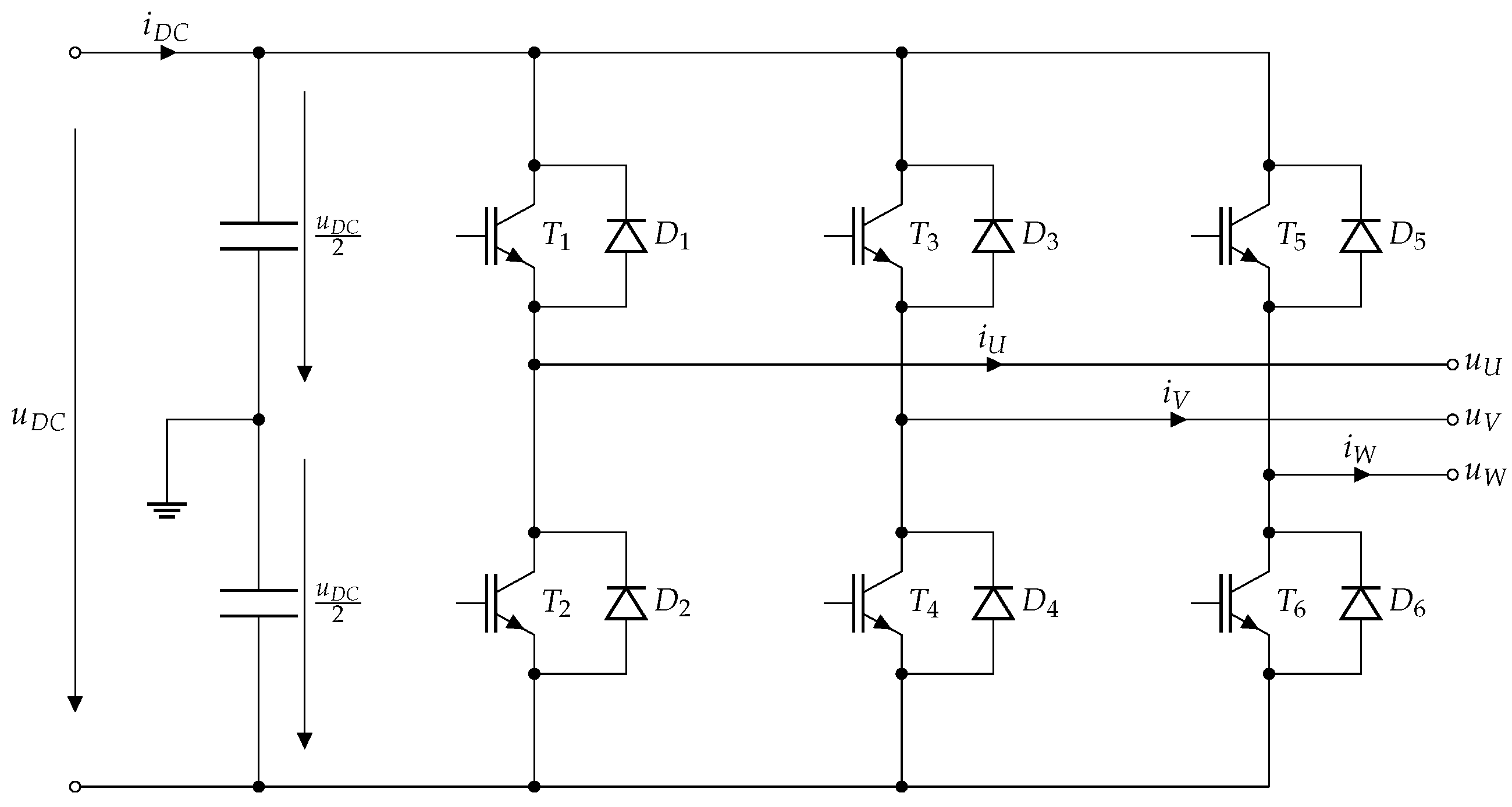
In the proposed system, a Voltage Source Inverter (VSI) is used. The equivalent circuit diagram of the power electronics is outlined in Figure 8. The AC side of the inverter is composed of an Insulated Gate Bibolar Transistor (IGBT) full bridge with an anti-parallel free-wheeling diode on each IGBT device. The output terminal voltages u U , u V and u W , with their corresponding currents i U , i V and i W , represent the interface to the electric drive. In order to generate a frequency and amplitude variable AC voltage from the DC-link voltage, the IGBTs must be switched, according to a defined pattern, using Pulse Width Modulation (PWM). Due to this switching pattern, the losses in the inverter consist of conduction and switching losses that depend on the used modulation scheme [46], which is a sine modulation with zero offset to improve the voltage utilization [47]. Due to the symmetric structure of the inverter, the loss behavior of the semiconductors differs only with a shift in time. Thus, the power dissipation models can be reduced to one IGBT and one diode, which are applied for all semiconductors afterwards.

3.2.1. Conduction Losses

Calculation of the conduction losses is carried out for the IGBT and diode pair T 1 , D 2 from Figure 8. The forward characteristics of the used power electronics are shown in Figure 9. The power loss caused by the nonlinear resistive behavior of the semiconductors can be described using a second-order phase current-dependent polynomial [48,49]
p ˜ c , T 1 = a c , T ( ϑ j , T ) · i T 1 + b c , T ( ϑ j , T ) · i T 1 2
p ˜ c , D 2 = a c , D ( ϑ j , D ) · i D 2 + b c , D ( ϑ j , D ) · i D 2 2 ,
with a c , T ( ϑ j , T ) , b c , T ( ϑ j , T ) and a c , D ( ϑ j , D ) , b c , D ( ϑ j , D ) as IGBT and diode junction temperature-dependent fitting coefficients.
The conduction power losses also depend on the modulation method or, respectively, on the relative conduction periods of each IGBT and diode during one commutation interval [46]. The used sine modulation with zero offset can be approximated by adding third-order harmonics to the standard sine modulation, which leads to the relative turn on times
β T 1 = 1 2 + M 1 2 cos ( φ e l ) + M 3 2 cos ( 3 φ e l )
β D 2 = 1 2 M 1 2 cos ( φ e l ) M 3 2 cos ( 3 φ e l ) ,
where M 1 and M 3 are the corresponding modulation indices and φ e l describes the phase angle between the current and voltage in one inverter leg. Assuming the currents to be sinusoidal without higher-order harmonics, the conduction losses for the used modulation scheme can be described by
P c , T 1 = a c , T ( ϑ j , T ) I ^ N 2 1 π + M 1 4 cos ( φ e l ) + b c , T ( ϑ j , T ) I ^ N 2 1 8 + M 1 3 π cos ( φ e l ) + M 3 15 π cos ( 3 φ e l )
for the IGBT and in a similar manner for the diode with
P c , D 2 = a c , D ( ϑ j , D ) I ^ N 2 1 π M 1 4 cos ( φ e l ) + b c , D ( ϑ j , D ) I ^ N 2 1 8 M 1 3 π cos ( φ e l ) M 3 15 π cos ( 3 φ e l ) .

3.2.2. Switching Losses

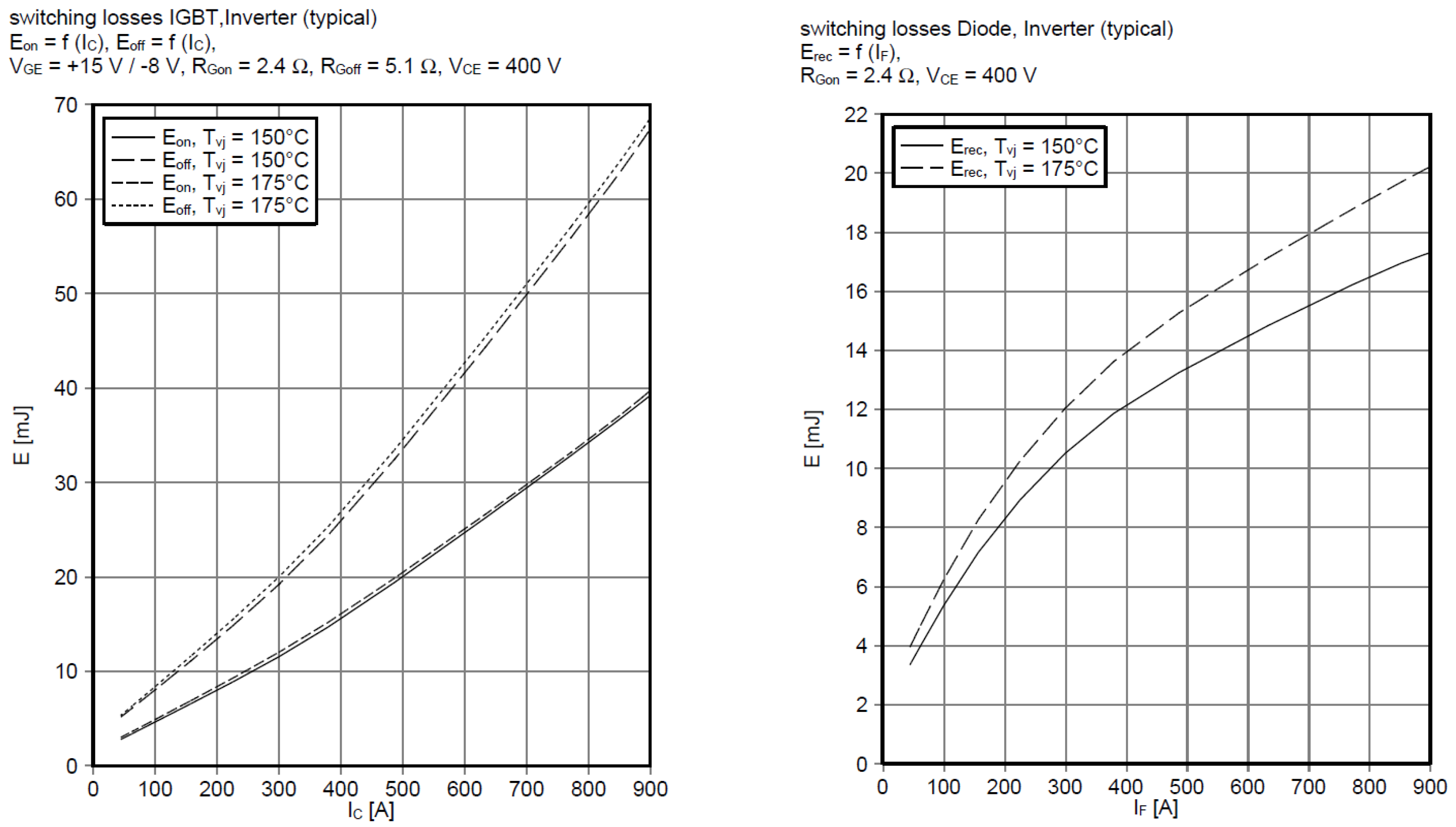
Caluclation of the switching losses is carried out in the same manner as the conduction losses for the IGBT and diode pair T 1 , D 2 . The switching losses of the IGBT occur during the transition from blocking to conducting state and vice versa. For the diode, the switching losses are mainly related to the reverse recovery effect during the transition from conduction to blocking state. The energies for one switching event are given in the corresponding semiconductor data sheet, as outlined in Figure 10, for the used module. In [46,49,51], a linear dependence between the switching energy w s w , l i n and the actual phase current i U , in the form
w s w , l i n = k s w , T , D · i U ( φ e l )
is assumed. However, as depicted in Figure 10, neither the diode nor the IGBT behave linearly regarding their switching losses. Thus, a second-order polynomial equation of the form
w ˜ E o n , T 1 = a E o n · i U + b E o n · i U 2 + c E o n
w ˜ E o f f , T 1 = a E o f f · i U + b E o f f · i U 2 + c E o f f
w ˜ E r r , D 2 = a E r r · i U + b E r r · i U 2 + c E r r
is used to model the nonlinear behavior of the turn-on and turn-off energies w ˜ E o n , T 1 , w ˜ E o f f , T 1 of the IGBT and for the diode reverse recovery losses w ˜ E r r , D 2 . The used sine modulation scheme causes each semiconductor to switch once in each PWM duty cycle. Therefore, a linear relationship between the switching frequency f s and the switching power losses
p ˜ E o n , T 1 = w ˜ E o n , T 1 ( φ e l ) · f s
p ˜ E o f f , T 1 = w ˜ E o f f , T 1 ( φ e l ) · f s
p ˜ E r r , D 2 = w ˜ E r r , D 2 ( φ e l ) · f s
exists.
In addition to the polynomial fit, the temperature dependencies of the switching losses are also taken into account. Furthermore, the switching losses behave nonlinearly regarding the applied blocking voltage, which is in case of the VSI the DC-voltage u D C . Averaging the switching losses over one fundamental wave period and including the aforementioned temperature and blocking voltage dependencies leads to
P E o n , T 1 = f s u D C u r e f , T κ T 1 + α T ( ϑ j , T ϑ r e f , T ) c E o n 2 + a E o n I ^ N π + b E o n I ^ N 2 4
P E o f f , T 1 = f s u D C u r e f , T κ T 1 + α T ( ϑ j , T ϑ r e f , T ) c E o f f 2 + a E o f f I ^ N π + b E o f f I ^ N 2 4
P E r r , D 2 = f s u D C u r e f , D κ D 1 + α D ( ϑ j , D ϑ r e f , D ) c E r r 2 + a E r r I ^ N π + b E r r I ^ N 2 4
describing the averaged switching losses with respect to the amplitude of the applied phase current I ^ N , the actual junction temperatures of the IBGT ϑ j , T and the diode ϑ j , D and the applied DC-voltage u D C . The voltages u r e f , T and u r e f , D describe the specific working point voltage in the semiconductor data sheet for which the switching losses are measured. The exponents κ T and κ D express the nonlinear behavior of the blocking voltage to the switching losses.
For the proposed VSI with six IGBT and diode pairs, the overall power losses of the inverter can be calculated as
P i n v = 6 P c , T 1 + P c , D 2 + P E o n , T 1 + P E o f f , T 1 + P E r r , D 2 .

3.2.3. Thermal Model

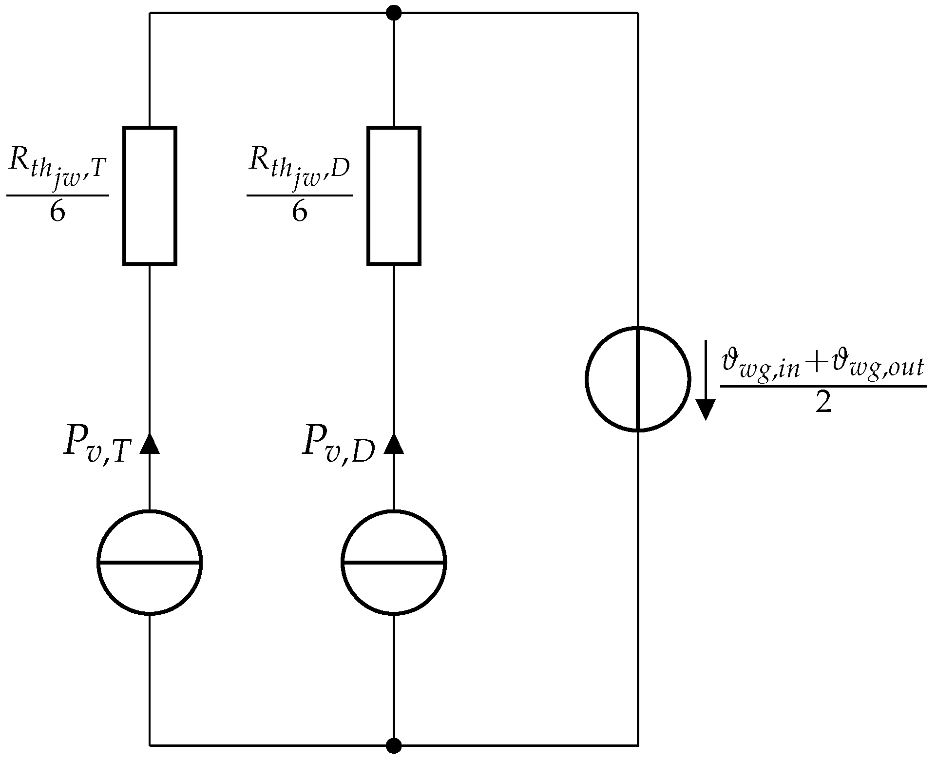
The thermal model of the water-cooled IGBT module is mainly defined by the thermal paths conducting heat from each IGBT and each diode to the cooling circuit. In the proposed thermal model, as outlined in Figure 11, cross-coupling effects between each semiconductor on the module are neglected. As the IGBTs and the diodes are loaded equally, the power losses P v , T and P v , D can be combined for all six semiconductors, leading to two heat dissipation sources. The heat is transferred to the cooling circuit by the thermal resistance R t h j w , T from the IGBT and by the thermal resistance R t h j w , D from the diode. The main advantage of equivalent circuit diagram models is the ease of parameterization of the models using the thermal impedances directly given in the data sheet [50]. Using the proposed model, the junction temperature of the semiconductors ϑ j , T and ϑ j , D can be calculated with
ϑ j , T = P v , T R t h j w , T 6 + ϑ w g
for the IGBTs and with
ϑ j , D = P v , D R t h j w , D 6 + ϑ w g
for the diodes, where ϑ w g denotes the temperature of the coolant. If channel flow characteristics [52] are assumed for the flow of the liquid coolant, the relation between the power dissipation of the semiconductors P v , T , P v , D , the coolant inlet and outlet temperatures ϑ i n , ϑ o u t and a given flow rate V ˙ w g can be expressed by
P v , T + P v , D = ρ w g ( ϑ w g ) V ˙ w g c p , w g ( ϑ w g ) ( ϑ o u t ϑ i n ) .
Due to the expected minor temperature increase between the inlet and outlet temperatures, the coolant temperature is assumed to be
ϑ w g = ϑ w g , i n + ϑ w g , o u t 2 .

3.3. EM Model

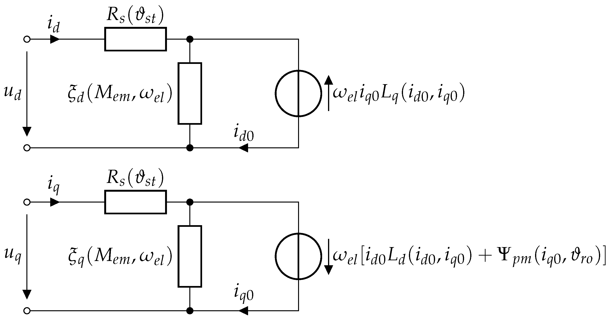
Modeling the permanent magnet synchronous machine (PMSM) is carried out using a fundamental wave model in d , q coordinates with saturation effects, as outlined in [53]. Furthermore, the model is expanded by nonlinear iron losses ξ d and ξ q introduced in [54]. As the time constant of the electrical drive is significantly smaller, in comparison to that of the mechanical system, the current dynamics in the model are neglected. This lead to the equivalent circuit models outlined in Figure 12 and the stationary machine equations [54]
u d = ( R s + ξ q L d ) i d ω e l L q i q + ξ q Ψ p m
u q = ( R s + ξ d L q ) i q + ω e l L d i d + ω e l Ψ p m
describing the electrical behavior of the drive in d , q coordinates. For the sake of simplicity and a better readability, the parameter dependencies are only outlined in the equivalent circuit model and not in the equations. As can be seen the parameters L d , L q and Ψ p m depend on the actual current working point i d 0 , i q 0 of the machine and caused by the saturation of the electrical drive. They were identified experimentally on a drive test-bench and are outlined in Figure 13. The dependencies of the iron losses ξ d and ξ q on the torque M e m and the velocity ω e l are shown in Figure 14. Furthermore, the copper resistance R s depends on the stator temperature ϑ s t , which can be described by
R s = R s , ϑ 0 [ 1 + α c u , ϑ 0 ( ϑ s t ϑ c u , 0 ) ] ,
where α c u , ϑ 0 is the temperature coefficient of copper and R s , ϑ 0 is the reference resistance at the reference temperature ϑ c u , 0 . The magnetic flux depends on the rotor temperature ϑ r o and can be described by
Ψ p m = Ψ p m , ϑ 0 [ 1 + α p m , ϑ 0 ( ϑ r o ϑ p m , 0 ) ] ,
where α p m , ϑ 0 is the temperature coefficient of the permanent magnet material and Ψ p m , ϑ 0 describes the reference magnetic flux at the reference temperature ϑ p m , 0 . The link between the electrical model and the corresponding air gap torque M a i r , taking the iron losses into account, can be described by [55]
M a i r = 3 2 p [ Ψ p m ( i q u q ξ q ω e l 2 L q ) + ( L d L q ) ( i d u d ξ d ω e l 2 L d ) ( i q u q ξ q ω e l 2 L q ) ] ,
with p denoting the number of pole pairs.

3.4. Environment Model

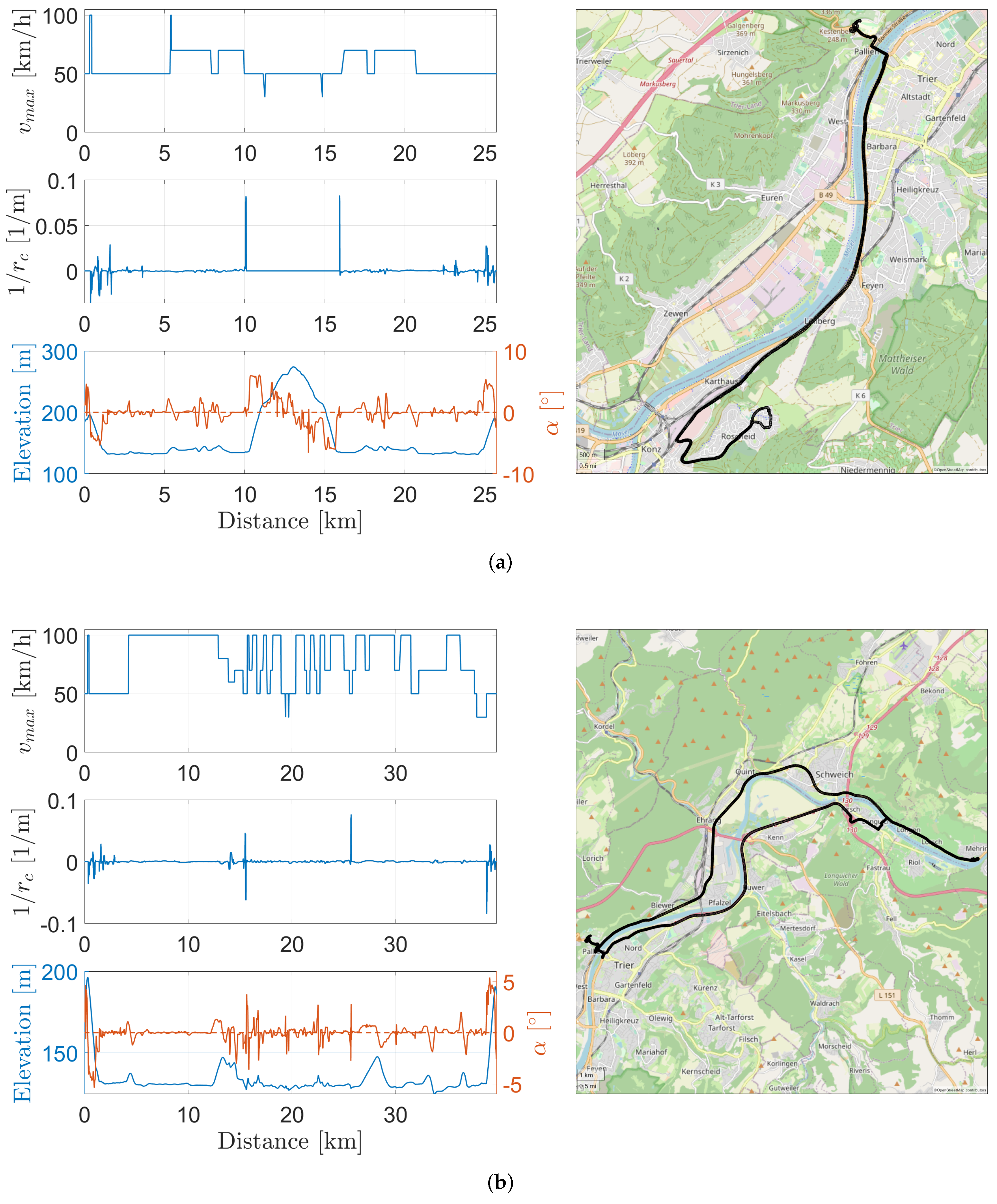
In order to use realistic driving scenarios for the vehicle defined in the previous sections, four different drive cycles were defined, which represent typical daily commuter routes to work in the urban and inter-urban areas around the German city Trier and are outlined in Figure 15 and Figure 16. The environment model describes the required route parameters of the driven route, including
  • Legal speed limit;
  • Curve radii;
  • Road slope and elevation.
The presented data were extracted from the HERE map database [56] for the given GPX tracks.
To account for the influence of commuting distances, all selected routes are of different length. Furthermore, it can be seen that the elevation profile is more distinct for drive cycles 1 and 2 than for drive cycles 3 and 4, thus covering the influence of different elevation profiles. Furthermore, the speed profiles of the drive cycles are also different. As can be seen, the legal speed limit v m a x for the drive cycles 1–3 is slower than that for drive cycle 4. It is important to mention that the start and end points of the route are at the same altitude. This avoids the insertion or extraction of potential energy of the system and thus, falsification of the results of the proposed sensitivity analysis.

4. Longitudinal Economic MPC

In the following, the longitudinal economic model predictive controller (EMPC) used to control the BEV is presented. Modern energy-efficient longitudinal motion controllers use information about the environment, such as route data [4]. Normally, the route information is provided by the map data provider as a function of the vehicle position. To process the data directly in the prediction, the proposed controller is discretized over position, rather than time. The domain change is performed using the relation [4,57]
d d t = d d s d s d t = d d s v .
Given the longitudinal motion model described in (A1)–(A9) and the transformation in (57), the velocity of the vehicle can be expressed as
d d s v e g o = M e m i g r w c r m v g cos ( α ) m v g sin ( α ) 1 2 ρ a i r c w A v e g o 2 m e q v e g o ,
as the first state of the controller design. The battery energy E b is used as the second state, which is given by
d d s E b = U o c v i b n c e l l v e g o .
Here, the open circuit voltage U o c v is assumed to be constant during the prediction. The battery current i b can be determined using
P D C ( M e m , v e g o ) + P p t o = i b n c e l l ( U o c v u R C 1 i b R s ) ,
where P D C ( M e m , v e g o ) denotes the DC power requested by the inverters and P p t o outlines the power needed by auxiliary consumers. This leads to
i b = n c e l l ( U o c v u R C 1 ) 2 R s n c e l l n c e l l ( n c e l l ( u R C 1 U o c v u R C 1 2 u o c v 2 ) + 4 R s ( P p t o + P D C ( M e m , v e g o ) ) ) 2 R s n c e l l
for the battery current. To ensure real-time capability and thus, practical applicability of the controller, the complex and nonlinear behavior of the drive and inverter is not transferred directly into the controller, as this would result in an overly complex controller design. Therefore, the DC power, as outlined in Figure 17a, is approximated using a second-order polynomial of the form
P D C ( M e m , v e g o ) 227.2 1.12 M e m + 60.04 v e g o + 0.3696 M e m 2 + 20.67 v e g o M e m + 1.206 v e g o 2 .
the voltage drop u R C 1 is calculated by
d d s u R C 1 = i b C 1 u R 1 C 1 R 1 v e g o
and serves as the third system state for the controller design. As outlined in Section 3.1.1 the parameters R 1 and C 1 are dependent on the working point. Nevertheless, the parameters are assumed to be constant over the prediction horizon as the working point, especially as the battery temperature and SoC, change only slowly. To keep the controller simple, only the dominant RC element of the battery is considered.
According to (58)–(63), the nonlinear state space model can then be fully described by
d d s v e g o E b u R C 1 = M e m i g r w c r m v g cos ( α ) m v g sin ( α ) 1 2 ρ a i r c w A v e g o 2 m e q v e g o U o c v i b n c e l l v e g o i b C 1 u R 1 C 1 R 1 v e g o ,
with
u = M e m
as the model input.
The energy efficiency control objective of the economic cost function
J ( x , u ) = 0 S p [ a c · ( v e g o ( s ) v r e f ) 2 + b c · ( M e m ( s ) M r e f ) 2 ] d s + c c · E b ( S p ) + d c · ( v e g o ( S p ) v r e f ) 2
is defined by the penalization c c of the utilized battery energy E b at the end of the prediction horizon S p within the Mayer term. However, considering only the battery energy would result in an unacceptable increase in driving time, due to the forced energy savings. To prevent this, the deviation from the reference velocity v r e f is penalized in the Mayer and Lagrange term. Furthermore, the deviation of the manipulated variable M e m to the required reference torque M r e f is penalized, in order to smoothen the controller response.
The maximum possible input torque M e m [ M m i n , M m a x ] is treated as a linear constraint. Furthermore, the power limitation caused by the maximum battery current, which results in a torque envelope for positive torques, as outlined in Figure 17b, is considered as a linear constraint of the form
M e m 97.01 2.173 v e g o .
Furthermore, the optimization problem should be bounded to ensure solvability and stability [58], which can be ensured by adding the constraints
5 300000 50 x ( s ) 30 300000 50 with s [ 0 , S p ]
to the optimization problem.
Equations (64)–(68) lead to the optimization problem
min u J ( x , u )
s . t . d d s x = f ( x , u )
x ( 0 ) = x 0
M m i n M e m ( s ) M m a x s [ 0 , S p ]
M e m ( s ) 97.01 2.173 v e g o ( s ) s [ 0 , S p ]
5 300000 50 x ( s ) 30 300000 50                                         s [ 0 , S p ] ,
which is discretized using a fourth-order Runge–Kutta algorithm and computed with the open-source framework acados [59].
The reference velocity v r e f is subject to two conditions. First, the maximum allowed legal speed v m a x , as already outlined in Figure 15, needs to be taken into account. Second, the maximum lateral acceleration a l , m a x allowed when driving a curve with the curve radius c r results also in a speed limit, which is defined by
v l , m a x = r c · a l , m a x .
The minimum of these two conditions would lead to the reference velocity v r e f . However, taking only the minimum may cause discontinuities to appear in the reference trajectory. To smoothen the reference trajectory, the discrete optimization problem [60]
min v s m o o t h i = 1 N p ( v r e f ( k + i | k ) v s m o o t h ( k + i | k ) ) 2
s . t . v s m o o t h ( k + i + 1 | k ) v s m o o t h ( k + i | k ) r m a x i { 1 , 2 , , N p }
v s m o o t h ( k + i | k ) v r e f ( k + i | k ) i { 1 , 2 , , N p } ,
with r m a x as the maximum allowed change of the optimization variable, is used over the prediction horizon N p .

5. Sensitivity Setup

To perform a suitable sensitivity analysis, the sensitivity setup needs to be defined, including the following information:
  • Which parameters are investigated;
  • The injection point of each parameter;
  • The distribution underlying each parameter;
  • The model outputs of interest.
For the proposed sensitivity analysis in this article, all investigated parameters are outlined in Table 1. They are arranged into groups, according to the components to which they belong. For the vehicle itself and its powertrain components, each parameter belongs to the parameters of the proposed models of Section 3. How the distributions are injected into the model and the types of error are also outlined in Table 1. Relative errors represent a percentage deviation of the nominal model values, whereas absolute errors directly describe the deviation of the parameter itself. The standard deviation σ for normally distributed parameters is mostly defined using the 3 σ values, representing the maximum error of the addressed parameter. As the objective of this investigation is to quantify the influences of the proposed parameters on the energy efficiency the outputs of interest are the combined power losses of all powertrain devices P l and the consumed battery energy E b . The combined power losses P l consider the battery, inverter, electric drive and gearbox losses. As the energy consumption of the vehicle is also influenced by the average driving speed, the required driving time t d , as an indicator of the average driving speed, is also taken into account.
The first step is to conduct a Morris screening of the proposed model, controller and parameter setup. Afterwards, the results provided by the Morris screening are used to exclude unimportant parameters from the quantitative sensitivity analysis, in order to reduce the computational time of the Monte-Carlo setup. The results of the proposed sensitivity analysis are outlined in the following chapter.

6. Simulation Results

In this chapter, the results of the sensitivity analysis are discussed. In Section 6.1, the results of the Morris screening are presented while, in Section 6.2, the outcomes of the quantitative variance-based sensitivity analysis are discussed.

6.1. Morris Screening

The results of the Morris screening for the four different drive cycles are outlined in Figure 18, Figure 19, Figure 20 and Figure 21. In general, it can be seen that the required battery energy E b behaves more linearly than the power losses P l throughout all driving cycles, as σ μ * holds. As σ is not negligibly small, compared to μ * , for the parameter dependencies of the power losses P l , nonlinear interactions between parameters can be assumed. Furthermore, it can be seen for both outputs E b and P l , that only a small subset of parameters have high values of μ * or σ compared to the rest of the parameters. Consequently only these parameters are taken into account in the variance-based sensitivity analysis. The remaining parameter set is outlined in Table 2.

6.2. Sobol Indices

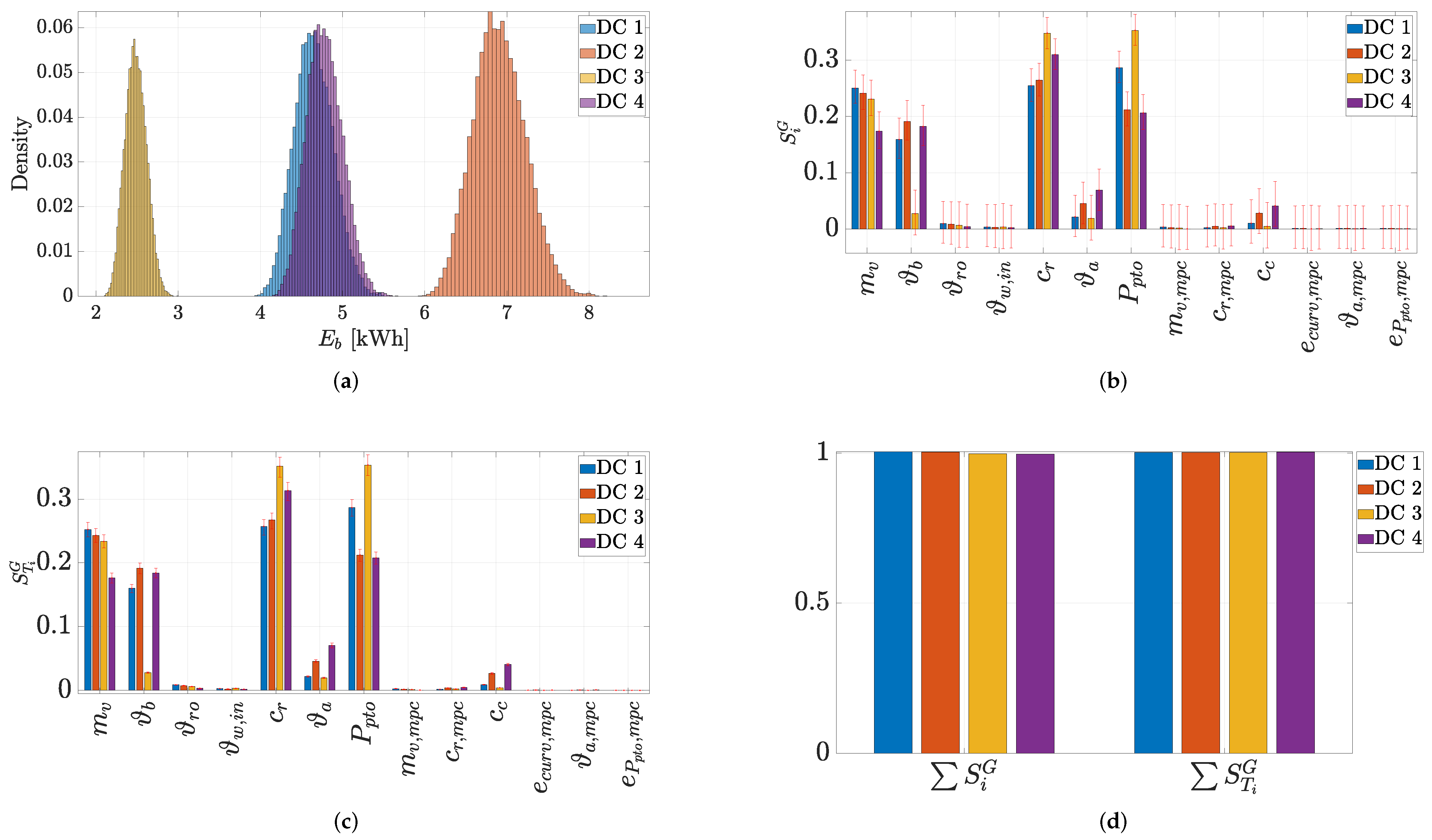
Figure 22a outlines the histograms of the required battery energy E b , caused by the parameter distributions outlined in Table 2, for the four different drive cycles. First of all, it can be seen that the average energy consumption varies for the drive cycles which is expected as they had different lengths and route profiles. Furthermore, it is evident that the examined parameters cause a significant variance in the required battery energy. As shown in Figure 22d S i G S T i G holds for all four drive cycles which indicates a linear parameter dependency on the output E b . This coincides with the qualitative Morris screening as already discussed in Section 6.1. Furthermore, it indicates that S i G S T i G , which means that the total and first-order effects are nearly equal. The first-order indices, as outlined in Figure 22b, show that only a few parameters are dominating the output variance. These are the rolling resistance coefficient c r , the auxiliary losses P p t o , the vehicle mass m v and the battery temperature ϑ b . Another important finding is that the parameter belonging to the controller—and thus, can be influenced during the operation of the vehicle—only contributes a maximum of 5% to the overall variance. In other words, it can be confirmed that operating or pre-conditioning the battery in a suitable temperature range and reducing the mass of the vehicle has much stronger effect on the energy consumption than tuning the parameters in an advanced control concept. However, the controller tuning parameter c c can be used to affect the energy consumption most from the point of view of the control strategy. It is also important to mention that the sensitivities of the driving cycles do not differ greatly and that the vehicle behaves relatively similarly. One exception is the sensitivity of the battery temperature ϑ b in drive cycle 3. This can be explained by the fact that less total energy or average power is converted in this drive cycle. Therefore, the ohmic battery losses and their dependence on the energy consumption do not have such a strong effect than for the other drive cycles.
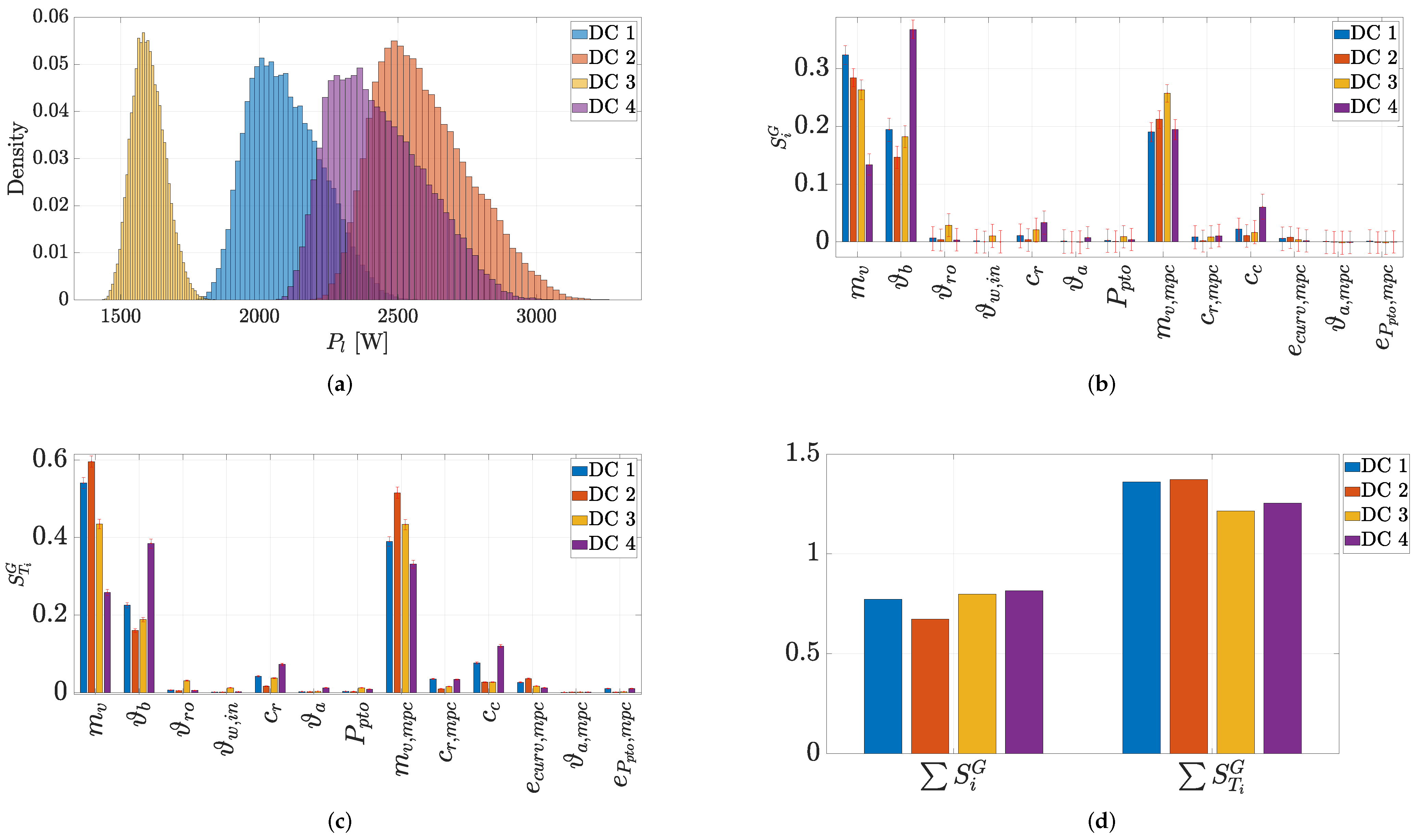
The next analyzed output of interest is P l , which combines all losses occurring in the powertrain during operation. As can be seen from Figure 23a, the investigated parameters have a significant influence on the variance of P l . The fact that S i G S T i G holds for all drive cycles, as depicted in Figure 23d, underpins the results of the Morris screening in Section 6.1 that nonlinear or higher-order effects exists. From Figure 23d it can be inferred that approximately 80% of the variance are caused by first-order and the rest by nonlinear or interaction effects.
The first-order effects of the power losses are shown in Figure 23b. Here, the vehicle mass m v and the the battery temperature ϑ b contribute significantly to the variance. However, beside the parameters related to the vehicle itself, it can be seen that the power losses are also influenced by the distribution of the estimated vehicle mass m v , m p c . This parameter is considered as a measured or estimated controller input variable. In this case, a reduction in the variance of m v , m p c could reduce the variance in the power losses significantly. In other words, if m v , m p c is better estimated or measured, the variance in the power losses. is also reduced The choice of c c also influence the power losses but the effect of this controller tuning parameter is rather small, compared to the parameters mentioned before.
Another interesting output to look at is the total driving time t d . This has a direct impact on the acceptance of a driver assistance system, as drivers are normally not willing to accept large increases in travel time. It can be seen that the investigated input parameters also caused a distribution of the driving time for the longitudinal control system as outlined in Figure 24a. The driving time behaves nearly linearly, as S i G S T i G holds, as outlined in Figure 24d. The nonlinear effects are negligibly small.
As the first-order effects of Figure 24b demonstrate, c c has the biggest influence on the driving time in drive cycles 2 and 4 which are the most energy-consuming drive cycles. However, as outlined above, the controller parameter c c has only a small effect on the energy consumption. Consequently, the travel time is mainly affected by c c without consuming significantly more or less energy. Meanwhile, aside from c c , the controller parameters m v , m p c and c r , m p c also have a significant influence on the driving time. Furthermore, the two vehicle parameters m v and c r clearly contribute to the distribution of t d .
To summarize the above outlined results, it can be stated that only a few of the investigated parameters have a notable impact on the analyzed output. Nevertheless, this influence is significant and clearly visible in the variances of the output and could not be neglected. Overall, that the most important parameters belonging to the vehicle or its components are the vehicle mass m v , the rolling resistance coefficient c r and the battery temperature ϑ b . From this, it is obvious that reducing the rolling resistance coefficient and also the mass of the vehicle will have a significant impact on the energy required by the vehicle. It is also shown that the battery temperature ϑ b also plays an important role, regarding the energy efficiency of the powertrain. Influencing the battery temperature during operation is not directly possible, as the thermal mass of the battery is so big that the battery losses would cause a major temperature rise to heat up the battery. However it can be seen, from our investigation, that a possible solution could be to pre-condition the battery before driving the vehicle, in order to reduce energy losses in the battery system.
Furthermore, it is outlined that the controller parameters have less impact on the energy consumption than the vehicle parameters, but they also have energy-saving potential. It can be seen, especially from the driving time t d , that the parameter c c has a large influence. Additionally, on the other outputs, an influence could be considered, which leads to the assumption that c c mainly affects the driving time, but it may possibly improve the energy consumption. It is also found that the measured or estimated mass of the vehicle m v , m p c and the rolling resistance c r , m p c cause a substantial amount of the variance in the driving time t d , as well as that in the power losses P l . As a consequence, these parameters should be estimated as accurately as possible, in order to improve the energy efficiency of the controller.
It is important to mention that the sensitivity analysis was performed for the controller proposed in Section 4. Thus, it is possible that, if the controller concept is modified, e.g., by changing the cost function or the constraints, the sensitivity analysis results will be affected. Similarly, the vehicle design can affect the results. For instance, with a heavier vehicle, the change in mass due to the number of people carried does not strongly affect the total mass much, in percentage terms. However, optimization of the vehicle is beyond the scope of this work.
It can be summarized that the investigated outputs behave differently regarding their parameter sensitivities. It should also be mentioned that the ranking, according to their importance, depends highly on the investigation or development target. The main interesting variables in this study for energy-efficient longitudinal motion control are the battery energy E b and the driving time t d . In contrast, if component loss optimization is the main development goal, the overall power losses P l or some component-specific losses (e.g., battery losses), should be the main variables of interest. Due to this difference in prioritization, depending on the development goal, the model outputs of interest should be considered separately and not evaluated together.

7. Conclusions

In this article, a novel approach for analyzing complex closed-loop economic model predictive longitudinal control systems is presented. It is outlined that a qualitative screening method is able to generate a reduced set of parameters for variance-based sensitivity analysis, thus reducing the computational burden of the Monte-Carlo simulation. The use of Generalized Sobol Indices outlined the ability to deal with time-dependent processes. It is shown that only a small subset of the parameters are sensitive regarding the energy consumption, the power losses and the driving time. It can be concluded that the vehicle mass, the battery temperature and the rolling resistance of the vehicle have the biggest influence on the energy consumption of the modeled vehicle, whereas the influence of EMPC tuning factors is only small with the unpleasant side-effect of worsening the driving time. Furthermore, it is shown that good estimates in the EMPC of the vehicle mass and the rolling resistance could improve the controller performance by reducing the variance of the energy consumption and driving time. In general the used methods can be seen as powerful tools for quantifying the effects on an output of the system with respect to their cause. This will help researchers or developers to identify relevant parameters and focus on them to more effectively improve the overall system behavior.

Author Contributions

Conceptualization, M.B.; methodology, M.B.; software, M.B.; validation, M.B., M.S. and H.V.; formal analysis, M.B.; investigation, M.B.; resources, M.B.; data curation, M.B.; writing—original draft preparation, M.B.; writing—review and editing, M.B., M.S. and H.V.; visualization, M.B.; supervision, M.S. and H.V. All authors have read and agreed to the published version of the manuscript.

Funding

This research received no external funding.

Institutional Review Board Statement

Not applicable.

Informed Consent Statement

Not applicable.

Data Availability Statement

The data presented in this study are available on request from the corresponding author.

Conflicts of Interest

The authors declare no conflict of interest.

Abbreviations

The following abbreviations are used in this manuscript:
ANOVAAnalysis of variance
BEVBattery electric vehicle
EMPCEconomic model predictive control
HDMRHigh-dimensional model representation
IGBTInsulated gate bipolar transistor
MPCModel predictive control
NMPCNonlinear model predictive control
PMSMPermanent magnet synchronous machine
PWMPulse width modulation
SoCState of charge
VSIVoltage source inverter

Appendix A

Appendix A.1. Longitudinal Motion Model

The longitudinal motion model considers the mechanical forces acting on a vehicle’s center of gravity and a gearbox model transforming the mechanical energy of the electric drives to the wheels. The force equilibrium in the center of gravity of the vehicle is described by
F L + F R = F a + F r + F s + F a i r ,
where F L and F R are the forces acting on the left and right rear wheel which drive the vehicle. The driving resistance forces comprise the acceleration resistance force F a , the rolling resistance force F r , the slope resistance force F s and the air resistance force F a i r . The acceleration resistance force is caused by Newton’s second law. It is expressed by
F a = m e q · a e g o ,
where m e q denotes the equivalent mass, including the inertia of the rotating parts of the powertrain which belong to their kinetic energy. Furthermore, a e g o describes the acceleration of the vehicle. The rolling resistance can be described by
F r = c r · m v · g · cos ( α ) with v e g o > 0 ,
where c r denotes the rolling resistance coefficient and α is the road slope angle. In a similar manner, the resistance force caused by the road slope
F s = m v · g · sin ( α )
describes the additional force when driving up or downhill, with g being the gravitational constant. Additionally, the movement of the vehicle through the surrounding air causes the aerodynamic resistance force
F a i r = 1 2 c w · A v · ρ a i r · v e g o 2
to act on the vehicle. This includes the aerodynamic drag coefficient c w , the frontal area of the vehicle A v and the air density ρ a i r .
The conversion from the longitudinal motion model and the associated forces to the rotational model of the powertrain is achieved by the law of levers. The transformation from the longitudinal driving forces F L and F R to the corresponding drive shaft torques M L and M R of the wheels is given by
M L = F L · r w
and
M R = F R · r w
with the wheel radius r w . Assuming, that the same torque is applied on the left and the right wheel the needed driving force in (A1) can be described by
F R + F L = M L + M R r w = 2 M D with M W = M L = M R .
The gearbox is modeled with a constant gear ratio i g , using a working point dependent efficiency map η g ( ω m , M e m ) . This leads to
M D = M e m · i g · η g ( ω m , M e m ) ,
describing the transition from the mechanical torque of the electrical drives M e m to the torques M D applied to the wheels. The parameters for the longitudinal motion model are provided in Table A1.
Table A1. Longitudinal motion model parameters.
ParameterDescriptionValue
c w Air drag coefficient0.262
A v Frontal area2.036 m2
m v Vehicle mass550 kg
m e q Equivalent vehicle mass (including rotational inertia)569 kg
r w Wheel radius0.283 m
i g Gear ratio5.85

References

  1. Jayakumar, A.; Chalmers, A.; Lie, T.T. Review of prospects for adoption of fuel cell electric vehicles in New Zealand. IET Electr. Syst. Transp. 2017, 7, 259–266. [Google Scholar] [CrossRef]
  2. Vaezipour, A.; Rakotonirainy, A.; Haworth, N. Reviewing In-vehicle Systems to Improve Fuel Efficiency and Road Safety. Procedia Manuf. 2015, 3, 3192–3199. [Google Scholar] [CrossRef]
  3. Barkenbus, J.N. Eco-driving: An overlooked climate change initiative. Energy Policy 2010, 38, 762–769. [Google Scholar] [CrossRef]
  4. Schwickart, T.; Voos, H.; Hadji-Minaglou, J.R.; Darouach, M.; Rosich, A. Design and simulation of a real-time implementable energy-efficient model-predictive cruise controller for electric vehicles. J. Frankl. Inst. 2015, 352, 603–625. [Google Scholar] [CrossRef]
  5. Schwickart, T.; Voos, H.; Hadji-Minaglou, J.R.; Darouach, M. A Fast Model-Predictive Speed Controller for Minimised Charge Consumption of Electric Vehicles. Asian J. Control. 2016, 18, 133–149. [Google Scholar] [CrossRef]
  6. Naus, G.; Ploeg, J.; van de Molengraft, M.; Heemels, W.; Steinbuch, M. Design and implementation of parameterized adaptive cruise control: An explicit model predictive control approach. Control Eng. Pract. 2010, 18, 882–892. [Google Scholar] [CrossRef]
  7. Jia, Y.; Jibrin, R.; Itoh, Y.; Görges, D. Energy-Optimal Adaptive Cruise Control for Electric Vehicles in Both Time and Space Domain based on Model Predictive Control. IFAC-PapersOnLine 2019, 52, 13–20. [Google Scholar] [CrossRef]
  8. Kamal, M.A.S.; Mukai, M.; Murata, J.; Kawabe, T. Model Predictive Control of Vehicles on Urban Roads for Improved Fuel Economy. IEEE Trans. Control Syst. Technol. 2013, 21, 831–841. [Google Scholar] [CrossRef]
  9. Caldas, K.A.Q.; Grassi, V. Eco-cruise NMPC Control for Autonomous Vehicles. In Proceedings of the 19th International Conference on Advanced Robotics (ICAR), Belo Horizonte, Brazil, 2–6 December 2019; IEEE: New York, NY, USA, 2019; pp. 356–361. [Google Scholar] [CrossRef]
  10. Chen, Y.; Li, X.; Wiet, C.; Wang, J. Energy Management and Driving Strategy for In-Wheel Motor Electric Ground Vehicles with Terrain Profile Preview. IEEE Trans. Ind. Inform. 2014, 10, 1938–1947. [Google Scholar] [CrossRef]
  11. Weißmann, A.; Görges, D.; Lin, X. Energy-Optimal Adaptive Cruise Control based on Model Predictive Control. IFAC-PapersOnLine 2017, 50, 12563–12568. [Google Scholar] [CrossRef]
  12. Sajadi-Alamdari, S.A.; Voos, H.; Darouach, M. Nonlinear model predictive extended eco-cruise control for battery electric vehicles. In Proceedings of the 24th Mediterranean Conference on Control and Automation (MED), Athens, Greece, 21–24 June 2016; IEEE: New York, NY, USA, 2016; pp. 467–472. [Google Scholar] [CrossRef] [Green Version]
  13. Vajedi, M.; Azad, N.L. Ecological Adaptive Cruise Controller for Plug-In Hybrid Electric Vehicles Using Nonlinear Model Predictive Control. IEEE Trans. Intell. Transp. Syst. 2016, 17, 113–122. [Google Scholar] [CrossRef]
  14. Frezza, G.; Evangelou, S.A. Ecological Adaptive Cruise Controller for a Parallel Hybrid Electric Vehicle. In Proceedings of the European Control Conference (ECC), St. Petersburg, Russia, 12–15 May 2020; IEEE: New York, NY, USA, 2020; pp. 491–498. [Google Scholar] [CrossRef]
  15. Sajadi-Alamdari, S.A.; Voos, H.; Darouach, M. Risk-averse Stochastic Nonlinear Model Predictive Control for Real-time Safety-critical Systems. IFAC-PapersOnLine 2017, 50, 5991–5997. [Google Scholar] [CrossRef]
  16. Sajadi-Alamdari, S.A.; Voos, H.; Darouach, M. Fast stochastic non-linear model predictive control for electric vehicle advanced driver assistance systems. In Proceedings of the IEEE International Conference on Vehicular Electronics and Safety (ICVES), Vienna, Austria, 27–28 June 2017; IEEE: New York, NY, USA, 2017; pp. 91–96. [Google Scholar] [CrossRef] [Green Version]
  17. Sajadi-Alamdari, S.A.; Voos, H.; Darouach, M. Nonlinear Model Predictive Control for Ecological Driver Assistance Systems in Electric Vehicles. Robot. Auton. Syst. 2019, 112, 291–303. [Google Scholar] [CrossRef] [Green Version]
  18. Moser, D.; Waschl, H.; Kirchsteiger, H.; Schmied, R.; del Re, L. Cooperative adaptive cruise control applying stochastic linear model predictive control strategies. In Proceedings of the European Control Conference (ECC), Linz, Austria, 15–17 July 2015; IEEE: New York, NY, USA, 2015; pp. 3383–3388. [Google Scholar] [CrossRef]
  19. Moser, D.; Schmied, R.; Waschl, H.; del Re, L. Flexible Spacing Adaptive Cruise Control Using Stochastic Model Predictive Control. IEEE Trans. Control Syst. Technol. 2018, 26, 114–127. [Google Scholar] [CrossRef]
  20. Morris, M.D. Factorial Sampling Plans for Preliminary Computational Experiments. Technometrics 1991, 33, 161–174. [Google Scholar] [CrossRef]
  21. Sobol, I.M. Sensitivity Analysis for Nonlinear Mathematical Models. Math. Model. Comput. Exp. 1993, 1, 407–414. [Google Scholar]
  22. Vepsäläinen, J.; Ritari, A.; Lajunen, A.; Kivekäs, K.; Tammi, K. Energy Uncertainty Analysis of Electric Buses. Energies 2018, 11, 3267. [Google Scholar] [CrossRef] [Green Version]
  23. Vepsäläinen, J.; Otto, K.; Lajunen, A.; Tammi, K. Computationally efficient model for energy demand prediction of electric city bus in varying operating conditions. Energy 2019, 169, 433–443. [Google Scholar] [CrossRef]
  24. Asamer, J.; Graser, A.; Heilmann, B.; Ruthmair, M. Sensitivity analysis for energy demand estimation of electric vehicles. Transp. Res. Part Transp. Environ. 2016, 46, 182–199. [Google Scholar] [CrossRef]
  25. Zhao, S.; Howey, D.A. Global Sensitivity Analysis of Battery Equivalent Circuit Model Parameters. In Proceedings of the IEEE Vehicle Power and Propulsion Conference (VPPC), Hangzhou, China, 17–20 October 2016; IEEE: New York, NY, USA, 2016; pp. 1–4. [Google Scholar] [CrossRef] [Green Version]
  26. Grandjean, T.R.B.; Li, L.; Odio, M.X.; Widanage, W.D. Global Sensitivity Analysis of the Single Particle Lithium-Ion Battery Model with Electrolyte. In Proceedings of the IEEE Vehicle Power and Propulsion Conference (VPPC), Hanoi, Vietnam, 14–17 October 2019; IEEE: New York, NY, USA, 2019; pp. 1–7. [Google Scholar] [CrossRef] [Green Version]
  27. Braband, M.; Adams, M.; Wilhelmi, A.; Scherer, M. Global Sensitivity Analysis on the Torque Accuracy of the Powertrain in Electric Vehicles. IFAC-PapersOnLine 2020, 53, 14067–14072. [Google Scholar] [CrossRef]
  28. Asef, P.; Lapthorn, A. Overview of Sensitivity Analysis Methods Capabilities for Traction AC Machines in Electrified Vehicles. IEEE Access 2021, 9, 23454–23471. [Google Scholar] [CrossRef]
  29. Saltelli, A.; Aleksankina, K.; Becker, W.; Fennell, P.; Ferretti, F.; Holst, N.; Li, S.; Wu, Q. Why so many published sensitivity analyses are false: A systematic review of sensitivity analysis practices. Environ. Model. Softw. 2019, 114, 29–39. [Google Scholar] [CrossRef]
  30. Alexanderian, A.; Gremaud, P.A.; Smith, R.C. Variance-based sensitivity analysis for time-dependent processes. Reliab. Eng. Syst. Saf. 2020, 196, 106722. [Google Scholar] [CrossRef] [Green Version]
  31. Campolongo, F.; Saltelli, A. Sensitivity analysis of an environmental model: An application of different analysis methods. Reliab. Eng. Syst. Saf. 1997, 57, 49–69. [Google Scholar] [CrossRef]
  32. Campolongo, F.; Tarantola, S.; Saltelli, A. Tackling quantitatively large dimensionality problems. Comput. Phys. Commun. 1999, 117, 75–85. [Google Scholar] [CrossRef]
  33. Campolongo, F.; Cariboni, J.; Saltelli, A. An effective screening design for sensitivity analysis of large models. Environ. Model. Softw. 2007, 22, 1509–1518. [Google Scholar] [CrossRef]
  34. Saltelli, A.; Annoni, P.; Azzini, I.; Campolongo, F.; Ratto, M.; Tarantola, S. Variance based sensitivity analysis of model output. Design and estimator for the total sensitivity index. Comput. Phys. Commun. 2010, 181, 259–270. [Google Scholar] [CrossRef]
  35. Homma, T.; Saltelli, A. Importance measures in global sensitivity analysis of nonlinear models. Reliab. Eng. Syst. Saf. 1996, 52, 1–17. [Google Scholar] [CrossRef]
  36. Gamboa, F.; Janon, A.; Klein, T.; Lagnoux, A. Sensitivity analysis for multidimensional and functional outputs. Electron. J. Stat. 2014, 8, 575–603. [Google Scholar] [CrossRef]
  37. Doyle, M.; Fuller, T.F.; Newman, J. Modeling of Galvanostatic Charge and Discharge of the Lithium/Polymer/Insertion Cell. J. Electrochem. Soc. 1993, 140, 1526–1533. [Google Scholar] [CrossRef]
  38. Fuller, T.F.; Doyle, M.; Newman, J. Simulation and Optimization of the Dual Lithium Ion Insertion Cell. J. Electrochem. Soc. 1994, 141, 1–10. [Google Scholar] [CrossRef] [Green Version]
  39. Krewer, U.; Röder, F.; Harinath, E.; Braatz, R.D.; Bedürftig, B.; Findeisen, R. Review—Dynamic Models of Li-Ion Batteries for Diagnosis and Operation: A Review and Perspective. J. Electrochem. Soc. 2018, 165, A3656–A3673. [Google Scholar] [CrossRef]
  40. Zhao, R.; Kollmeyer, P.J.; Lorenz, R.D.; Jahns, T.M. A Compact Methodology Via a Recurrent Neural Network for Accurate Equivalent Circuit Type Modeling of Lithium-Ion Batteries. IEEE Trans. Ind. Appl. 2019, 55, 1922–1931. [Google Scholar] [CrossRef]
  41. Chiasserini, C.F.; Rao, R.R. Energy efficient battery management. IEEE J. Sel. Areas Commun. 2001, 19, 1235–1245. [Google Scholar] [CrossRef]
  42. Hageman, S.C. Simple PSpice models let you simulate common battery types. Electron. Des. News 1993, 38, 117–129. [Google Scholar]
  43. Hentunen, A.; Lehmuspelto, T.; Suomela, J. Time-Domain Parameter Extraction Method for Thévenin-Equivalent Circuit Battery Models. IEEE Trans. Energy Convers. 2014, 29, 558–566. [Google Scholar] [CrossRef]
  44. Hamm, P. Thermische Charakterisierung und Evaluierung einer LiFePO4-Batteriezelle. Master’s Thesis, University of Applied Sciences, Trier, Germany, 2021. [Google Scholar]
  45. Lehnertz, M. Entwicklung eines Schätzverfahrens zur Bestimmung der Inneren Zelltemperatur von LiFePO4 Batteriezellen. Master’s Thesis, University of Applied Sciences, Trier, Germany, 2021. [Google Scholar]
  46. Kolar, J.W.; Ertl, H.; Zach, F.C. Influence of the modulation method on the conduction and switching losses of a PWM converter system. IEEE Trans. Ind. Appl. 1991, 27, 502–512. [Google Scholar] [CrossRef]
  47. Schröder, D. Elektrische Antriebe—Regelung von Antriebssystemen, 4th ed.; Springer: Berlin/Heidelberg, Germany, 2015. [Google Scholar] [CrossRef]
  48. Drofenik, U.; Kolar, J.W. A general scheme for calculating switching-and conduction-losses of power semiconductors in numerical circuit simulations of power electronic systems. Proc. IPEC 2005, 5, 4–8. [Google Scholar]
  49. Bierhoff, M.H.; Fuchs, F.W. Semiconductor losses in voltage source and current source IGBT converters based on analytical derivation. In Proceedings of the IEEE 35th Annual Power Electronics Specialists Conference, Aachen, Germany, 20–25 June 2004; IEEE: New York, NY, USA, 2004; pp. 2836–2842. [Google Scholar] [CrossRef]
  50. Infineon Technologies AG. HybridPACK Drive Module FS820R08A6P2: Final Data Sheet, V3.3; Infineon Technologies: Neubiberg, Germany, 2019. [Google Scholar]
  51. Windisch, T.; Hofmann, W. Energieeffiziente Regelung von Fahrzeugantrieben mit permanenterregten Synchron- und Asynchronmotoren unter Berücksichtigung von Umrichter, Eisenverlusten und Sättigung. In Elektrische Antriebstechnologie Für Hybrid-Und Elektrofahrzeuge; Schäfer, H., Ed.; Springer: Berlin/Heidelberg, Germany, 2019; pp. 218–237. [Google Scholar]
  52. Baehr, H.D.; Stephan, K. Wärme-Und Stoffübertragung, 8th ed.; Springer: Berlin/Heidelberg, Germany, 2013. [Google Scholar] [CrossRef]
  53. Schröder, D. Elektrische Antriebe—Grundlagen, 5th ed.; Springer: Berlin/Heidelberg, Germany, 2013. [Google Scholar] [CrossRef]
  54. Kellner, S.L.; Seilmeier, M.; Piepenbreier, B. Impact of iron losses on parameter identification of permanent magnet synchronous machines. In Proceedings of the 1st International Electric Drives Production Conference, Nuremberg, Germany, 28–29 September 2011; IEEE: New York, NY, USA, 2011; pp. 11–16. [Google Scholar] [CrossRef]
  55. Kellner, S.L. Parameteridentifikation bei Permanenterregten Synchronmaschinen. Ph.D. Thesis, University of Erlangen-Nuremberg, Erlangen, Germany, 2012. [Google Scholar]
  56. HERE Technologies. HERE Plattform. Available online: https://www.here.com/platform (accessed on 22 January 2022).
  57. Kohut, N.J.; Karl Hedrick, P.J.; Borrelli, P.F. Integrating Traffic Data and Model Predictive Control to Improve Fuel Economy. IFAC Proc. Vol. 2009, 42, 155–160. [Google Scholar] [CrossRef] [Green Version]
  58. Faulwasser, T.; Grüne, L.; Müller, M.A. Economic Nonlinear Model Predictive Control. Found. Trends® Syst. Control. 2018, 5, 1–98. [Google Scholar] [CrossRef]
  59. Verschueren, R.; Frison, G.; Kouzoupis, D.; Frey, J.; van Duijkeren, N.; Zanelli, A.; Novoselnik, B.; Albin, T.; Quirynen, R.; Diehl, M. acados—A modular open-source framework for fast embedded optimal control. Math. Program. Comput. 2022, 14, 147–183. [Google Scholar] [CrossRef]
  60. Schwickart, T.K. Energy-Efficient Driver Assistance System for Electric Vehicles Using Model-Predictive Control. Ph.D. Thesis, University of Luxembourg, Luxemburg, 2015. [Google Scholar]
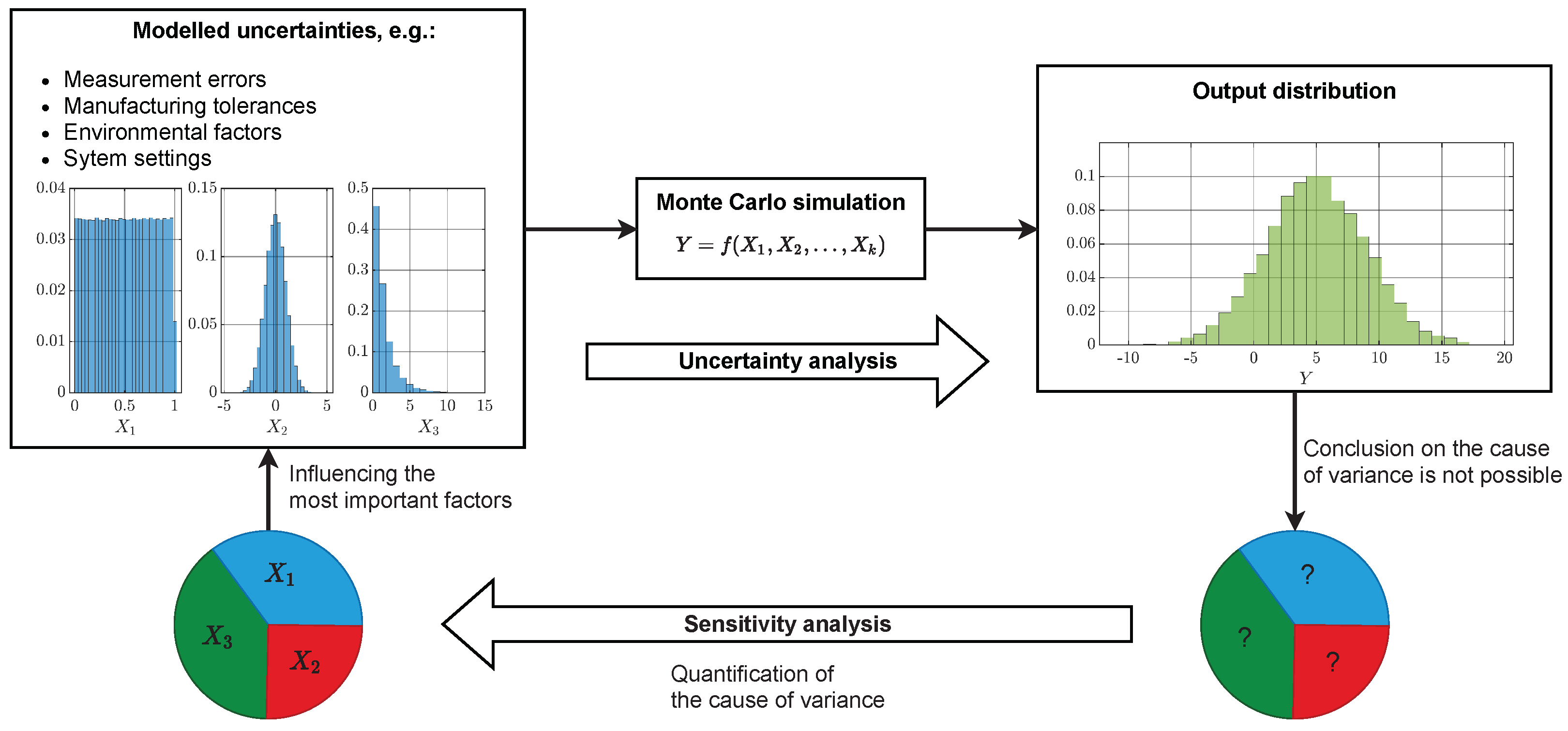
Figure 1. Process of a variance-based sensitivity analysis. The difference between an uncertainty analysis and a sensitivity analysis is also outlined.
Electronics 11 01574 g001
Figure 2. Sketch of the proTRon Evolution.
Electronics 11 01574 g002
Figure 3. Simulation setup of the proposed BEV.
Electronics 11 01574 g003
Figure 4. Electrical equivalent circuit model of the battery.
Electronics 11 01574 g004
Figure 5. Electrical battery parameters, according to [44]. (a) R s ; (b) R 1 ; (c) R 2 ; (d) C 1 ; (e) C 2 .
Electronics 11 01574 g005
Figure 6. Battery capacity and open circuit voltage, according to [44]. (a) Battery capacity; (b) Open circuit voltage.
Electronics 11 01574 g006aElectronics 11 01574 g006b
Figure 7. Thermal equivalent circuit model of the battery (a) 2D thermal model, (b) Equivalent circuit model.
Electronics 11 01574 g007
Figure 8. VSI equivalent circuit.
Electronics 11 01574 g008
Figure 9. Forward characteristics of the used IGBT module [50].
Electronics 11 01574 g009
Figure 10. Switching energies with respect to the load current of the used IGBT module [50].
Electronics 11 01574 g010
Figure 11. IGBT thermal equivalent circuit model.
Electronics 11 01574 g011
Figure 12. Saturation- and iron loss-dependent PMSM equivalent circuits.
Electronics 11 01574 g012
Figure 13. Working point-dependent drive parameters (a) Direct inductance L d , (b) Quadrature inductance L q , (c) Magnetic flux Ψ p m .
Electronics 11 01574 g013
Figure 14. Working point-dependent iron losses (a) Direct axis iron loss parameter ξ d , (b) Quadrature axis iron loss parameter ξ q .
Electronics 11 01574 g014
Figure 15. Drive cycle overview (a) Drive cycle 1, (b) Drive cycle 2.
Electronics 11 01574 g015
Figure 16. Drive cycle overview (a) Drive cycle 3, (b) Drive cycle 4.
Electronics 11 01574 g016
Figure 17. DC power map (a) without battery current limitation, (b) with battery current limitation.
Electronics 11 01574 g017
Figure 18. Morris screening for drive cycle 1 (a) Bat energy E b , (b) Power losses P l .
Electronics 11 01574 g018
Figure 19. Morris screening for drive cycle 2 (a) Bat energy E b , (b) Power losses P l .
Electronics 11 01574 g019
Figure 20. Morris screening for drive cycle 3 (a) Bat energy E b , (b) Power losses P l .
Electronics 11 01574 g020
Figure 21. Morris screening for drive cycle 4 (a) Bat energy E b , (b) Power losses P l .
Electronics 11 01574 g021
Figure 22. Generalized Sobol Indices and histograms for consumed battery energy E b (a) Histograms, (b) First-order effects with 95% confidence interval, (c) Total effects with 95% confidence interval, (d) Sum of effects.
Electronics 11 01574 g022
Figure 23. Generalized Sobol Indices and histograms for the total drive power losses P l (a) Histograms, (b) First order effects with 95% confidence interval, (c) Total order effects with 95% confidence interval, (d) Sum of effects.
Electronics 11 01574 g023
Figure 24. Generalized Sobol Indices and histograms for the total driving time t d (a) Histograms, (b) First-order effects with 95% confidence interval, (c) Total effects with 95% confidence interval, (d) Sum of effects.
Electronics 11 01574 g024
Table 1. Distributions of parameters for sensitivity analysis.
NameDescriptionType of ErrorDistributionParameterValuesUnits
Battery e R s , b Deviation of series resistance R s relativeNormal μ , σ 0, 0.05 / 3
e C 1 Deviation of capacitance C 1 relativeNormal μ , σ 0, 0.05 / 3
e R 1 Deviation of resistance R 1 relativeNormal μ , σ 0, 0.05 / 3
e C 2 Deviation of capacitance C 2 relativeNormal μ , σ 0, 0.05 / 3
e R 2 Deviation of resistance R 2 relativeNormal μ , σ 0, 0.05 / 3
e U o c v Deviation of open circuit voltagerelativeNormal μ , σ 0, 0.025 / 3
ϑ b Variation of start temperatureabsoluteUniforma, b20, 40°C
R t h c a Variation of thermal resistance R t h c a absoluteNormal μ , σ 2.6042 , 0.1302 / 3 Ω
R t h c t Variation of thermal resistance R t h c t absoluteNormal μ , σ 0.3682 , 0.0184 / 3 Ω
R t h t a Variation of thermal resistance R t h t a absoluteNormal μ , σ 1.0526 , 0.0526 / 3 Ω
C c Variation of thermal capacitance C c absoluteNormal μ , σ 2544.2 , 127.21 / 3 F
C t Variation of thermal capacitance C t absoluteNormal μ , σ 8.072 , 3.4036 / 3 F
Inverter e a t Deviation of forward characteristics IGBTrelativeNormal μ , σ 0, 0.02 / 3
e b t relativeNormal μ , σ 0, 0.02 / 3
e a d Deviation of forward characteristics dioderelativeNormal μ , σ 0, 0.02 / 3
e b d relativeNormal μ , σ 0, 0.02 / 3
e a E r r Deviation of reverse recovery
characteristics diode
relativeNormal μ , σ 0, 0.02 / 3
e b E r r relativeNormal μ , σ 0, 0.02 / 3
e c E r r relativeNormal μ , σ 0, 0.02 / 3
e a E o n Deviation of turn on losses IGBTrelativeNormal μ , σ 0, 0.02 / 3
e b E o n relativeNormal μ , σ 0, 0.02 / 3
e c E o n relativeNormal μ , σ 0, 0.02 / 3
e a E o f f Deviation of turn off losses IGBTrelativeNormal μ , σ 0, 0.02 / 3
e b E o f f relativeNormal μ , σ 0, 0.02 / 3
e c E o f f relativeNormal μ , σ 0, 0.02 / 3
ϑ w , i n Variation of water inlet temperatureabsoluteUniforma, b0, 50°C
Drive e R s , E M Deviation of winding resistance R s relativeNormal μ , σ 0, 0.03 / 3
e L d Deviation of direct inductance L d relativeNormal μ , σ 0, 0.0133 / 3
e L q Deviation of quadrature inductance L q relativeNormal μ , σ 0, 0.015 / 3
e Ψ p m Deviation of magnetic flux Ψ p m relativeNormal μ , σ 0, 0.025 / 3
e ξ q Deviation of quadrature iron losses ξ q relativeNormal μ , σ 0, 0.02 / 3
e ξ d Deviation of direct iron losses ξ d relativeNormal μ , σ 0, 0.02 / 3
ϑ r o Variation of rotor temperature ϑ r o absoluteUniforma, b40, 80°C
ϑ s t Variation of stator temperature ϑ s t absoluteUniforma, b40, 80°C
Vehicle m v Variation of the vehicle massabsoluteBirnbaum–Saunders β , γ 652.111 , 0.0742427 k g
P p t o Variation of auxiliary consumersabsoluteUniforma, b250, 750 W
ϑ a Variation of ambient temperatureabsoluteNormal μ , σ 12.261 , 8.52975 °C
p a i r Variation of ambient pressureabsoluteNormal μ , σ 98427.7 , 843.09 Pa
c r Variation of rolling resistanceabsoluteUniforma, b 0.01 , 0.015
Controller c c Energy related cost function parameterabsoluteUniforma, b0, 6-
ϑ a , m p c Error of ambient temperature measurementabsoluteNormal μ , σ 12.261 , 8.52975 °C
p a i r , m p c Error of air pressure estimationabsoluteNormal μ , σ 98427.7 , 843.09 Pa
c r , m p c Error of rolling resistance estimationabsoluteUniforma, b 0.01 , 0.015
m v , m p c Error of vehicle mass estimationabsoluteBirnbaum–Saunders β , γ 652.111 , 0.0742427 k g
e U o c v , m p c Error of open circuit voltage estimationrelativeNormal μ , σ 0, 0.05 / 3
e R s , m p c Error of battery series resistance estimationrelativeNormal μ , σ 0, 0.05 / 3
e R 1 , m p c Error of battery RC-resistance estimationrelativeNormal μ , σ 0, 0.05 / 3
e C 1 , m p c Error of battery RC-capacitance estimationrelativeNormal μ , σ 0, 0.05 / 3
e α , m p c Error of slope measurementrelativeNormal μ , σ 0, 0.05 / 3
e P p t o , m p c Error of auxiliary power estimationabsoluteUniforma, b250, 750 W
e c u r v , m p c Error of curvature measurementrelativeNormal μ , σ 0, 0.05 / 3
e S o C , m p c Error of SoC estimationrelativeNormal μ , σ 0, 0.10 / 3
e ϑ b , m p c Error of battery temperature estimationrelativeNormal μ , σ 0, 0.05 / 3
e I b , m p c Error of battery current measurementrelativeNormal μ , σ 0, 0.05 / 3
Table 2. Reduced parameter set for the variance-based sensitivity analysis.
NameDescriptionType of ErrorDistributionParameterValuesUnits
Battery ϑ b Variation of start temperatureabsoluteUniforma, b20, 40°C
Inverter ϑ w , i n Variation of water inlet temperatureabsoluteUniforma, b0, 50°C
Drive ϑ r o Variation of rotor temperature ϑ r o absoluteUniforma, b40, 80°C
Vehicle m v Variation of the vehicle massabsoluteBirnbaum–Saunders β , γ 652.111 , 0.0742427 k g
P p t o Variation of auxiliary consumersabsoluteUniforma, b250, 750 W
ϑ a Variation of ambient temperatureabsoluteNormal μ , σ 12.261 , 8.52975 °C
c r Variation of rolling resistanceabsoluteUniforma, b 0.01 , 0.015
Controller c c Energy related cost function parameterabsoluteUniforma, b0, 6-
ϑ a , m p c Error of ambient temperature measurementabsoluteNormal μ , σ 12.261 , 8.52975 °C
c r , m p c Error of rolling resistance estimationabsoluteUniforma, b 0.01 , 0.015
m v , m p c Error of vehicle mass estimationabsoluteBirnbaum–Saunders β , γ 652.111 , 0.0742427 k g
e P p t o , m p c Error of auxiliary power estimationabsoluteUniforma, b250, 750 W
e c u r v , m p c Error of curvature measurementrelativeNormal μ , σ 0, 0.05 / 3
Publisher’s Note: MDPI stays neutral with regard to jurisdictional claims in published maps and institutional affiliations.