A Proposed Waiting Time Algorithm for a Prediction and Prevention System of Traffic Accidents Using Smart Sensors

Abstract

One of the applications of neural networks is to predict the fault section results of traffic utilizing the combined model estimation of the fault section and self-learning models with smart sensors. The prediction of the fault section can autonomously develop the internal model of the network to fit the pre-entered “traffic accident” section data and predict the occurrence of traffic accident sections. In this paper, we propose the results of waiting time for traffic accidents in case of traffic accidents by using a neural network and fuzzy expert system, in comparison with existing algorithms and algorithms for determining traffic accidents. It is used to estimate or predict traffic accident reliability as well. Typically, the type of fault data collected is the number of faults (the number of faults recorded during a given time interval) or the time of fault (the time-of-fault data recorded when each fault occurred), and this can be utilized only for group data types, rather than the time-of-fault data type.

1. Introduction

Fuzzy logic allows for the inclusion of uncertain human assessments in computing problems by giving an effective method for conflict resolution of various criteria and better option assessment. The first research paper on fuzzy logic published in 1965 dealt with information originating from computational vision and cognition. Fuzzy-logic-based computing technologies help to create intelligent systems for decision making, identification, pattern recognition, optimization, and control. Engineers, mathematicians, software developers, natural scientists, medical researchers, and business analysts can benefit greatly from fuzzy logic [1].

Grouped data are data that have been bundled together in categories. Histograms and frequency tables are very useful to show these types of data: For instance, a relative frequency histogram shows book sales for a certain day, sorted by price. A frequency table shows data grouped by height. Fault data are placeholder data that represent managed data but are not fully realized yet or are a collection of data that represent a relationship: Managed fault data are appropriate classes of data, but their persistent variables still cannot be initialized.

Real-time traffic information on roads, information on accidents and construction, restaurants, petrol stations, theatres, and parks are among the services provided to smart-sensor-based drivers [2,3]. This article presents a technique to prevent traffic accidents by employing intelligent algorithms to identify parts of closed roads due to traffic accidents and other construction activities. Even well-designed intelligent electronic traffic lights cannot play the correct role at intersections during rush hour, when there are many vehicles, or when traveling via roads suspended due to severe calamities or construction. In this research, traffic data are processed by employing the method of determining the ideal signal period for junctions based on traffic information and telematics observed via a loop detector [4,5]. As an example, we can trace terrible road conditions by ice, snow, and rain on the road. Previous studies have employed telematics technology for traffic catastrophe broadcasting and real-time traffic forecasting systems in disaster areas for effective disaster broadcasting [2,6].

Fuzzy logic is able to manage both large and small traffic events well due to the effects of extreme weather scenarios that generally describe the fuzzy feature inaccurately. It is necessary to combine environmental aspects with several traffic metrics to be able to locate events on roads after working with the relationship between weather and the probability of mishaps. Neural networks, in addition to fuzzy logic, have indeed been established for the forecasting of traffic accidents and have efficiently been applied in a variety of transportation-related scientific disciplines, particularly safe driving, with superior efficiency. When it comes to predicting road accidents, artificial intelligence (AI) approaches such as ANNs can surpass all other techniques.

Recent articles [7,8,9,10,11,12,13,14,15,16] justify that the neural network suffers from the absence of a systematic method for determining the quantity or type of input vector values in forecasting future target values, as well as the fact that the model’s categorization is unclear. To overcome these drawbacks, researchers have attempted to establish symbolic classification rules in neural networks or produce interpretable interpretations using decision trees. Therefore, motivated by the above facts, we defined the goal of this study as to increase prediction accuracy by integrating an algorithm with a neural network algorithm and using the model’s data mining methods. Neural network methods are among the adaptable nonlinear models for addressing prediction problems in data with complicated structures in terms of data analysis. Initially, evacuees portray stochastic learning automata that choose an escape path based on physical characteristics and past evacuation decisions.

Typically, the type of fault data collected is the number of faults (the number of faults recorded during a given time interval) or the time of fault (the time of fault data recorded when each fault occurred), and this can be utilized for group data types, rather than the time-of-fault data type. Thus, we proposed the results of waiting time for traffic accidents by using “neural network” and “fuzzy expert system”. We utilized a combined estimation of the fault section and self-learning models using a smart sensor, to predict the occurrence of traffic accidents.

The main contributions of this work are as follows:

• We proposed a system to prevent traffic accidents by using intelligent algorithms to determine the sections where roads are bound to close due to traffic accidents and construction sites;
• We performed traffic data processing by calculating the optimal traffic cycle using a neural network;
• We improved the accuracy of prediction by combining the C4.5 algorithm with a neural network algorithm;
• We compared the results with existing algorithms for determining weather conditions such as heavy snow, fog, and freeze, and the resulting traffic accidents.

The rest of this paper is organized as follows: In Section 2, the processing of traffic data collection using electronic tags is described. We presented the road information analysis using an intelligent sensor network in Section 3. Section 4 presents the combining effect of the fault section and self-learning models. Section 5 presents a comparison of the proposed study with other studies. Section 6 illustrates the parameters for improving the traffic flow. Finally, Section 7 illustrates the conclusion of the study and provides suggestions for future research.

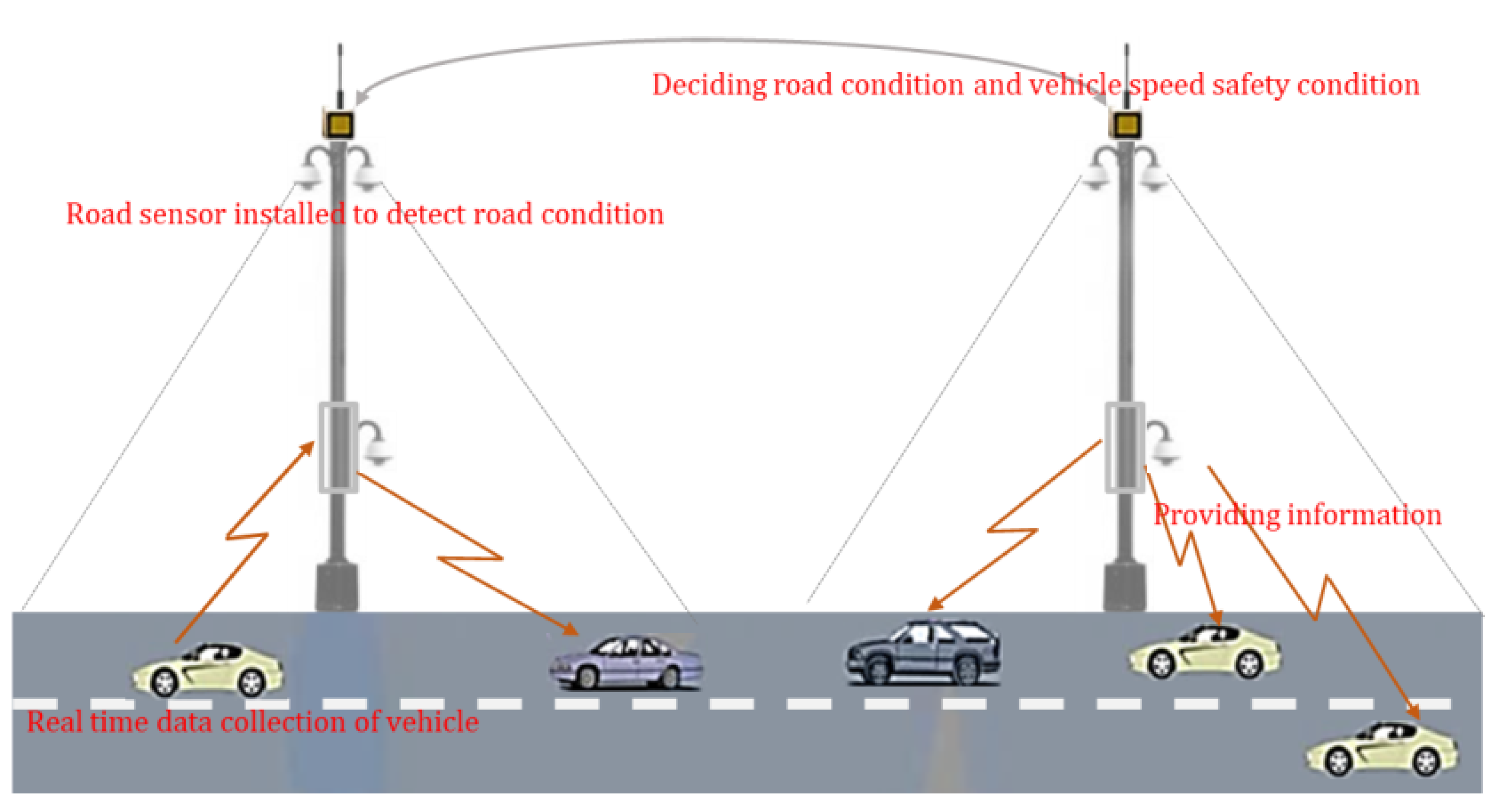
2. Traffic Data Collection Using Electronic Tags

Japan, North America, and northern Europe are commercializing intelligent “traffic accident prevention systems” through extensive research on automobiles and roads using telematics techniques in order to prepare for unexpected weather changes and various disasters such as traffic accidents, heavy fog, and heavy rain on roads. Regarding the process of obtaining the energy source of radio waves transmitted from tags, it is divided into passive and active types. Ubiquitous technology has been implemented in which roads are protected by ubiquitous technology for drivers’ safety by providing artificial intelligence to inanimate roads to melt ice by themselves [17,18,19,20]. During a passive process, transmission energy is acquired from radio waves received from the reader, whereas in an active process, transmission energy is acquired from a separate battery [17,18]. The intelligent road network informs the driver of fog and freezing conditions on the road using a road surface detection sensor as well as humidity and temperature sensors, as shown in Figure 1.

The purpose of this study is to extract the optimal traffic cycle using a neural network algorithm. In the field of data analysis, neural network algorithms can be classified as one of the flexible nonlinear models for solving prediction problems on data with complex structures. Because of its similarity with human neurophysiology, it is generally studied with greater research interest than other statistical prediction models. In particular, there are studies comparing the superiority of neural networks over logistic regression as a prediction technique [21]. However, neural networks have disadvantages. The model’s classification is ambiguous [22], and it lacks a systematic mechanism for identifying the quantity or kind of input vector values utilized in forecasting future target values. Researchers have sought to circumvent these disadvantages by establishing symbolic classification rules in neural networks or producing interpretable interpretations using decision trees [23].

The emergency survival camping and preparedness equipment (ESCAPE) service was developed based on the principles of reinforcement learning and game theory and executed at two decision-making layers. Initially, evacuees modeled stochastic learning automata that select an evacuation route that they want to go based on its physical characteristics and past decisions during the current evacuation. Consequently, according to [23], a cluster of evacuees is created per evacuation route, and the evacuees decide if they will finally evacuate through the specific evacuation route at the current time slot or not.

The objective of this research is to improve the accuracy of prediction by combining the C4.5 algorithm with a neural network algorithm, and we used data mining algorithms of the model. The authors of [24] proposed a method of selecting decision variables that meet the purpose of improving the accuracy of the overall classification model. However, the article [5] is strictly focused on performing the first task to form a C4.5 decision tree. This decision tree resembles a “divide-and-conquer” technique. In these techniques, the model forms a tree consisting of cases where one class belongs to all subsets so that the input training set can be successfully partitioned.

As a result, a cluster of evacuees is generated per evacuation route, and the evacuees select whether or not to escape by that route at the current time slot. The approach of picking choice variables that satisfy the goal of enhancing the overall classification model’s accuracy is discussed in [24].

The information profit ratio used as a basis for separating nodes is to separate the current training in a way that can reduce the average information required to categorize the given example. With the full training set |S|, if the current training set is S, and the number of (Case) in class Ci (i = 1, 2, … n) is Freq (Ci, S), then the average information required to identify a given class is given by Equation (1).

$$Info \left(S\right)={{\displaystyle \sum }}_{i=1}^n\frac{Freq \left(Ci, S\right)}{\left|S\right|}+=\log \left(2\right)(\frac{Freq \left(Ci, S\right)}{\left|S\right|})\times bis$$

(1)

where bis stands for the average information required for full training set |S| if the current training set is S, and the number of (Case) in class Ci (i = 1, 2, … n) is Freq (Ci, S).

From any test X, if S is separated into n subsets $S_1, S_2, \dots , S_n$, the information gained is found by Equation (2).

$$\mathrm{gain}\left(\mathrm{X}\right)=Info\left(S\right)-{{\displaystyle \sum }}_{i=0}^n\frac{S_i}{S}\times \mathrm{Info}\left(S_i\right)$$

(2)

Here, the information profit ratio is obtained using Equation (3).

$$\mathrm{gain}\left(X\right)=\frac{gain\left(X\right)}{splitInfo\left(X\right)}$$

(3)

3. Road Information Analysis via an Intelligent Sensor Network

At a road intersection, the traffic signal cycle becomes erroneous if the intersection situation cannot be correctly determined in various situations that make the intersection condition change significantly [7,8,9,10,11,12,13,14,15,16,17]. For example, in some cases, a sudden increase in traffic volume and blockage may occur due to random traffic accidents, construction work, an increase in a pedestrian crossing, various social and sports events such as a marathon, and increased traffic volume.

Generally, if the expected transit vehicle has less than 30–70% of the intersection capacity, it can generate an optimal traffic signal cycle by operating four signal phases—namely, north–south straight, right turn, left turn, and east–west straight. However, if the expected transit vehicle is a supersaturation with an intersection capacity of 90% or more, the traffic signal cycle should be reduced, and in particular, if some lanes are closed due to traffic accidents and other construction or events, the two signal phases (north–south straight and east–west straight) should be operated to shorten passenger waiting time. In this way, traffic information is converted every moment and is considered to guarantee a better traffic flow by sensing the speed of the vehicle using the GPS installed in the vehicle, analyzing the traffic flow, and immediately giving the optimum signal period [12].

Here, 20 intersection input and output values for calculating the optimal traffic signal cycle are displayed. As shown in

Table 1. Intelligent traffic signal cycle input and output values.

INPUT	NODE 1–2 REDUCE	NODE 1–2 EXTENSION	NODE 3–4 REDUCE	NODE 3–4 EXTENSION	NODE 5–6 REDUCE	NODE 5–6 EXTENSION	NODE 7–8 REDUCE	NODE 7–8 EXTENSION	NODE 9–10 REDUCE	NODE 9–10 EXTENSION
SATURATION UP BIG	BIG	SMALL	MED	SMALL	BIG	SMALL	BIG	SMALL	BIG	SMALL
SATURATION UP SMALL	BIG	SMALL	BIG	SMALL	MED	SMALL	BIG	SMALL	BIG	MED
PASSING UP SMALL	SMALL	SMALL	BIG	SMALL	BIG	MED	BIG	SMALL	BIG	SMALL
PASSING UP SMALL	BIG	MED	BIG	MED	MED	SMALL	BIG	MED	BIG	SMALL
SATURATION DN SMALL	BIG	SMALL	MED	SMALL	BIG	MED	BIG	SMALL	BIG	MED
SATURATION DN BIG	SMALL	SMALL	BIG	SMALL	BIG	SMALL	BIG	SMALL	BIG	SMALL
PASSING DN SMALL	BIG	MED	BIG	MED	MED	SMALL	BIG	MED	BIG	SMALL
PASSING DN BIG	SMALL	BIG	MED	SMALL	BIG	MED	BIG	SMALL	BIG	MED
PASSING PCU	MED	SMALL	BIG	BIG	BIG	SMALL	BIG	SMALL	BIG	SMALL
SPEED AND LENGTH DN	MED	MED	BIG	SMALL	MED	SMALL	BIG	MED	BIG	SMALL
SPEED AND LENGTH UP	MED	SMALL	BIG	SMALL	BIG	MED	BIG	SMALL	BIG	MED
SPILLBACK DOWN	MED	SMALL	BIG	SMALL	BIG	SMALL	BIG	SMALL	BIG	SMALL
SPILLABCK UP	BIG	SMALL	BIG	SMALL	BIG	SMALL	MED	SMALL	BIG	SMALL
DELAY UP	LOW	HIGH	MED	SMALL	MED	SMALL	MED	MED	MED	SMALL
DELAY DN	BIG	SMALL	BIG	SMALL	MED	SMALL	BIG	SMALL	MED	MED
LANES UP	BIG	SMALL	BIG	SMALL	BIG	SMALL	BIG	SMALL	BIG	SMALL
LANES DN	MED	BIG	MED	MED	MED	MED	MED	MED	MED	SMALL
BLOCK AREA	SMALL	SMALL	SMALL	SMALL	MED	SMALL	MED	SMALL	MED	SMALL
PHASE-1 UP	SMALL	BIG	MED	SMALL	MED	SMALL	MED	SMALL	MED	SMALL
PHASE-1 DN	BIG	BIG	BIG	MED	BIG	MED	BIG	MED	MED	MED

, even if there are many passing vehicles in the upper intersection, if the number of lanes in the sub-intersection is small and is in the supersaturated state, the optimum green time should be shortened, not lengthened [13,14]. From Table 1, it can be inferred that traffic is effectively distributed based on the generated signals, owing to the mentioned parameters in terms of their significance value ( low, medium, and high). There are 10 nodes (intersection and sub-intersection) that are considered for extended and reduced circumstances. Therefore, based on a particular input, a significance value (low, medium, and high) is assigned to nodes based on extended and reduced conditions. This provides clear information about the decisions to be taken under various scenarios for effective traffic management.

Equations (4)–(12) are used to determine the optimal signal cycle, taking into account disaster-related and traffic accident conditions that can occur at an intersection.

$$\mathrm{LostTimeG}1=\mathrm{Green}-1\left(\frac{1}{3\mathrm{Pg} }\right)+YellowTime\left(Pg+\frac{1}{2Py}\right)+RedTime(Pg+Py+\frac{1}{3}Pr)$$

(4)

$\mathrm{LostTimeG}1$

$$Gt2=Nveh\times 3+SDT$$

(5)

$$\mathrm{LostTimeG}2=\mathrm{Green}-1\left(\frac{1}{21\mathrm{Pg} }\right)+YellowTime\left(Pg+\frac{1}{2Py}\right)+RedTime(Pg+Py+\frac{1}{2}Pr)$$

(6)

$$Gt3=Nveh\times 3\times Cflane+SDT+RoadConversionTime$$

(7)

$$\mathrm{LostTimeG}3=\mathrm{Green}-1\left(\mathrm{Pg}\right)+YellowTime\left(Pg+\frac{1}{2Py}\right)+RedTime(Pg+Py+\frac{1}{2}Pr)$$

(8)

$$Gt4=Nveh\times 3\times \nabla ayTime$$

(9)

$$\mathrm{LostTimeG}4=\mathrm{Green}-1\left(\frac{1}{4\mathrm{Pg} }\right)+YellowTime\left(Pg+\frac{1}{4Py}\right)+RedTime(Pg+Py+\frac{1}{4}Pr)$$

(10)

$$Gt5=Nveh\times 3\times Cflane+SDT+RoadConversionTime$$

(11)

$$\mathrm{LostTimeG}5=\mathrm{Green}-1\left(\frac{1}{4\mathrm{Pg} }\right)+YellowTime\left(\frac{1}{3Pg}+\frac{1}{4Py}\right)+RedTime(\frac{1}{3Pg}+Py+\frac{1}{4}Pr)$$

(12)

The description of these notions is provided in what follows in

Table 2. Table of nomenclature.

$Gt1, Gt2\dots Gt5:$	Optimal green time considering interlocking
$Nveh:$	Number of passing vehicles
$CFLane:$	Lane compensation factor
$SDT:$	Set-off delay time
$RoadConversionTime:$	Intersection type compensation time
$LostTime:$	Passenger car standby time
$PG:$	Predicted green time (Probability of Green Time)
$PY:$	Predicted yellow time (Probability of Yellow Time)

.

Figure 2 illustrates the optimization process considering the preprocessing and postprocessing steps for intersection conditions, according to actual traffic conditions in cases such as a sudden increase or decrease in traffic volume, change from four-signal phases to two-signal phases, and closure of some lanes due to various road works or events [15,16].

Figure 3 shows the process of preventing traffic accidents by transmitting information through a smart-sensor-based driver system when the accident button information and current vehicle speed are transmitted to the traffic accident prevention system during a traffic accident while driving or when a sudden obstacle (i.e., accident vehicle) is found. Different methods have been developed for fault identification and diagnosis. The statistical algorithms applied for other related patterns are available in [25]. Similarly, using acoustic emission monitors and accelerometers facilitates the control of progressive levels, as indicated in [26]. The authors in [27] constructed a linear model to predict the wear and breakage of devices. However, it is very difficult to apply the linear model to industrial processes due to its nonlinear nature. Neural networks generally model tools for unknown functions. Scholars in [28] used a neural network to estimate the unidentified process of cutting through online learning, and subsequently, a nonlinear observer was designed using the developed neural network model. Nevertheless, the states are identified, and in our approach, we utilized two neural networks for designing the system. The first neural network was utilized to learn the system’s features when it is running correctly. The second neural network was utilized for developing a diagnostic technique for the detection of nonlinear faults in the system. Some unknown parameters such as the weights of neural networks, found in [29], were used to modify the learning rules. The final obtained model utilized a state observer to monitor the working of the system. The workflow of the system is explained below.

We started by introducing the concept of incipient fault and abrupt fault. Then, the second neural network utilized an estimator to estimate the faults. The equation describing the system is depicted below [29].

In Figure 3, RSE stands for remote single-layer embedded.

Let us consider a fault function for the system as described below:

$$\begin{gathered} a=M_v+N[ f\left(p,q\right)+G\left(s-S\right)\left(p,q\right)] \\ b=D_v^s \end{gathered}$$

(13)

where $\mathrm{G}\left(\mathrm{s}-\mathrm{S}\right)=\left\{\begin{array}{c}0\\ 1 \\ 1\end{array}-e^{-\gamma \left(s-S\right) }\right.\begin{array}{c}s<S\\ s\ge S\end{array}$. where $\varnothing \left(p,q\right)\in x^2$ is a vector that represents the fault in the system. $G\left(s-S\right)\in x^2$ shows the time profile of fault. $\gamma >0$ is an unknown constant that shows the rate at which the fault occurs, and S is the time of occurrence of the fault.

When a nonlinear function $\varnothing \left(p,q\right)$ is unidentified, the fault function becomes unavailable. However, the function $\varnothing \left(p,q\right)$ will become smooth only when the following condition is satisfied:

$$\varnothing \left(p,q\right)={\beta }^s\theta \left(p,q\right)+\varnothing$$

(14)

where $\varnothing \left(p,q\right)$ is a fault function with approximation error bounded $\varnothing$ hold true $\left|\varnothing \right|\le {\varnothing }_j$. The ideal weight is

$$W=\alpha \gamma {\left(\min \right)}_{we} \beta y\sup \left(p,q\right)\in \beta y|w^s\theta \left(p,q\right)-\varnothing \left(p,q\right)$$

(15)

where approximation error bounded $\varnothing$ holds true $\left|\varnothing \right|\le {\varnothing }_j$. Here, the magnitude is dependent on the basis of function choice and the number of nodes. Let us consider an estimated model as follows:

$$\widehat{\mathrm{A}}=N\left[\widehat{Q}S\theta \left(\widehat{p}q\right)\right]+x\left[m-D^{SAp}\right)+G\widehat{\varnothing }\left(\check{p},q,\widehat{w}\right)$$

(16)

where $\widehat{\varnothing }$ is a neutral network, and $\widehat{w}$ shows the weight of the network.

$$\widehat{\varnothing }\left(\widehat{p}q\right)={\widehat{W}}^s\theta \left(\widehat{p}, q\right)$$

(17)

where weight $\widehat{W}$ depicts an online tuning algorithm. The development of a suitable estimation method is a key element in the development of a scheme for fault diagnosis. The performance of the nonlinear estimation model above utilizes to treat device failures in an adaptive manner. For a better understanding of the system, consider a second-order, nonlinear system [29].

$$\begin{gathered} a=\left[\begin{array}{cc}1& 0\\ 0& 1\end{array}\right]m+\left[\begin{array}{c}5\\ 1\end{array}\right]\left[n-11y_{1}si{n}^2\left(m_1\right)\right] \\ b=\left[1 0\right]m \end{gathered}$$

(18)

$$G\left(s-3\right)\varnothing \left(p\right)=\left(1-e^{-0.6\left(s-3\right)}\right)p_2^2$$

(19)

The gain-of-observer control is selected as R = [200, 10] S to satisfy the surface plasmon resonance (SPR) state. The number of nodes utilized in the neural network model is 10. The observer monitors fault detection. Thus, the second neural network is activated for estimating the function of the fault. From these equations, it is clear that the second neural network remains zero before a fault occurs and changes to a specific value after the fault occurs.

Algorithm 1: Traffic accident prevention algorithm

INPUT:

int safety = max (st_path- > d_curve0, st_path- > d_curve1);

int length = max (st_path- > distance0, st_path- > distance);

int capacity = MAX (st_path- > capt0, st_path- > - > capt1);

intcan_work = MAX (st_path- > work0, st_path- > work1);

/* Read Traffic Conditions */

for (y = 0; y < min (trf_condition, distance); y++)

for (y = 0; y < MIN (trf_condition, distance); y++)

{

traffic_con (capacity, buf1 [distance0]);

traffic_con (capacity, buf2 [distance1]);

/* extract the sets from the fuzzy values */

Ax = f1- > x;

Ay = f1- > y;

Adistance = f1- > n;

Bx = f2- > x;

Ay = f2- > y;

Bdistance = f2- > n;

if (Alength == 1 andand Blength == 1)

{

if (Ay [0] < By [0])

{

if (DoIntersect) * intersectionSet = CopyFuzzyValue (f1);

return(Ay [01]);

}

else

{

if (DoIntersect) * intersectionSet = CopyFuzzyValue (f1);

return (Ay [01];

}

else

{

if (DoIntersect) * intersectionSet = CopyFuzzyValue (f2);

Return (By [0]);

}

}

if (Alength == 1)

{

max = By [0];

for (i = 1; i < Bdistance; i++)

if (By [i] > max) max = By [i];

if (max < Ay [0])

{

if (DoIntersection) * intersectionSet = CopyFuzzyValue (f2);

}

else

{

max = Ay [0];

if (DoIntersection) * intersectionSet = horizontal_intersection (f2, max);

}

return (max);

}

if (Blength == 1)

{

max = Ay [0];

for (i = 1; i < Adistance; i++)

if (Ay [i] > max) = Ay [i];

if (max < By [0])

{

if (DoIntersection) * intersectionSet = CopyFuzzyValue (f1);

}

else

if (nrandom == YES)

if (n_c < 3)

nfval++;

switch (n_c)

{

case 0: /* small car */

{

ncar [0]++

break;

}

case 1: /* medium car */

{

ncar [1]++;

break;

}

case 2: /* large car */

{

ncar [2]++;

break;

}

/* check for traffic condition */

if ((pass1 + pass2) > 140)

{

weight = random (5000) + 25,000;

outtextxy (48,090, “High Capacity.”);

}

else if ((pass1 + pass2) > 130

{

weight = random (5000) + 22,500;

outtextxy (48,090, “LOW Capacity.”);

}

else if ((pass1 + pass2) > 120)

{

weight = random (5000) + 17,500;

outtextxy (48,090, “Middle Capacity.”);

}

else if ((pass1 + pass2) > 100)

{

weight = random (5000) + 12,500;

outtextxy (48,090, “High Speed”);

}

else if ((pass1 + pass2) > 80)

{

weight = random (5000) + 7500;

outtextxy (48,090, “Middle Capacity.”);

}

else

{

weight = random (8000);

outtextxy (48,090, “Low speed”);

}

sprintf (buffer3, “%d”, weight);

outtextxy (55,075, buffer3);

OUTPUT

As shown in Figure 4 and Figure 5, the smart sensor applies the intelligent fuzzy algorithm to the road surface state data (the degree of moisture and temperature measured from the road) for controlling the maximum speed of the road ( Figure 6) while reading from the RFID to generate a rule (as in Figure 7). These data become input values for driver service and intelligent traffic-signal processing to generate optimized signal periods.

From Figure 7, we can infer that factors such as temperature, water level, and speed are dependent on one another, and some inference may be drawn on how drivers can tune the speed of their vehicle based on road temperature and humidity content to avoid accidents. As depicted in Figure 7, when the temperature is not very high (T < 4), speed is usually high (S > 5), and as the temperature increases (T > 4), the speed of the driver is reduced (S < 5). Similarly, the speed is high (S > 5) when the water level is low (W < 6), and it decreases rapidly (S < 4) once the level of water on the road is high (W > 6). Therefore, it is clear that both water level (humidity) and temperature are considered in parallel while increasing or decreasing the speed.

In order to use traffic data that change in real time as information, data on a traffic situation are immediately stored in the database to judge the traffic flow. This allows the analysis of the traffic flow in the driving direction of the driver and can provide drivers with traffic information to reach their destination more quickly and safely.

The location and speed of vehicles are periodically sensed by the smart sensor. Examples of real-time information include information about waiting vehicles during a signal period, information on how many cars are proceeding on the road and in which direction, and information about which traffic accident occurred at which intersection, and which point is under construction. When we input this type of information, it is possible to know how much time is required for the driver to pass the section in the near future, and how to give traffic signals to speed up the vehicle flow.

Figure 8 shows the configuration of the sensor database system. The system collects traffic situation data in real time, and the collected information is immediately stored in the database. If the user requests forecast information for the near future using our proposed algorithm, traffic flow information is provided by calculating the estimated time in real time using the information of local variables (traffic accidents, road repair work, etc.) requested by the driver. The first neural network model is used to calculate a non-zero variable. It is necessary to obtain this variable since it varies from time to time relative to other known constants and is a critical function in deciding to what extent the system will vary from the nominal output. Since the time varies, the input used for the first neural network is time, and the residual values have the greatest sensitivity to affect the system. The performance generated from neural network training is used for predicting the system’s “ideal” state. The second neural network is the “threshold logic generation network” that uses the output obtained from the previous neural network to create faulty conditions for creating a new compensated system. It would allow for greater precision in detecting faults. In addition, it ensures the provision of a properly defined state space for defective conditions. The third network is used to identify and diagnose faults. However, it is possible to obtain the fault magnitude of every ineffective sensor and actuator from each residual. The system’s feedback loop eventually causes each residual to affect the system.

4. Combining Fault Section and Self-Learning Models

4.1. Value of Sensors

Outliers, stuck-at faults, and spikes are detected with the help of statistics. Variables include sensor X, current value Ci, and previous n values in the current window (Y = Cn-I + Cn-I + 1 + Cn-I + 2………….Ci). We can also define the set of m windows with the same length as G = C1, C2,…………………Cm. Then, we can predict the value in each window through Gaussian distribution. If Φ2n = 0, then a stuck-at fault occurs. If Φ2n = infinity, then a spike fault may occur [28].

$$y_k=f\left(\alpha ,{\varnothing }^2\right)$$

(20)

where $\alpha ={\displaystyle \sum }_{j=1}^i{\mu }_j$ and ${\varnothing }^2=\frac{{{\displaystyle \sum }}_{j=1}^i{\left({\mu }_j-\alpha \right)}^2}{i}$.

In front of the current window, there is a buffer. For the latest samples being inputted to the current slot, a part of the obsolete samples acts as the buffer. When the current window size reaches I, the oldest window is discarded, and the current window joins the oldest window. Using the statistical sliding window method, large numbers of historical sensor values are regressed to j pairs of Gaussian attributes. We do not need to keep any of the recent values in memory in a specific program.

4.2. Status of Groups

Sensors are not in the same group on the opposite side of a valve. A valve is a common IoT controller. The proper valve can shut down all of the devices at the rear position. The sensors on different sides could be in different conditions. When one valve monitors so many sensors, they divide into separate classes. In our strategy, we did not use more than 10 sensors in one status category because, with the growing numbers of sensors, the possible state area sharply increases. For this case, sensors should be associated with the most complex system by their relative location, since the simpler system more likely results in a shift in status.

4.3. Model Status

The model divides according to the geographical location. However, the relationship between the sensors is out of the scope of our study and, hence, ignored. All the sensors in a group can function in different patterns. A sensor’s pattern can be determined from a particular size of the state-change window to suit its values. Here, we used the least-square method [30] to match the values and report the sensor index to the logical pattern matrix. In this method, the main concept of a gradual clustering algorithm is used to treat pattern vectors, respectively, to obtain the cosine angle between the new trend and existing vectors. If the angle is too wide, then a new phenomenon emerges. Otherwise, there is a repeated trend, and we only need to fuse it with the nearest vector. Consider the equations below [21].

$$\widehat{p}=A+B\widehat{Z}$$

(21)

where $A=\frac{\sum p}{m}-\frac{\varnothing \sum \widehat{Ƶ}}{m}$ and $B=\frac{m\sum p\widehat{Ƶ}-\sum p\sum \widehat{Ƶ}}{m\sum z^2-{\left(\sum \widehat{Ƶ}\right)}^2}$.

4.4. Computational Analysis Summary

In summary, we used the least-square method [30] to match the values and report the sensor index to the logical pattern matrix. The main concept of a gradual clustering algorithm is used to treat pattern vectors, respectively, to obtain the cosine angle between the new trend and existing vectors. The fault detection has been depicted in Figure 9.

5. Comparison with Other Works

Accident count analysis was effectively performed by using statistical approaches such as the Poisson, negative binomial, and derivatives in univariate and multivariate regression models [31], which aimed to resolve evidence and statistical problems relevant to assessments and forecasts of traffic injuries and strengthen our knowledge of the interaction between the factors and results of accidents. The literature on current traffic safety suggests that the predictive analysis applied fails when dealing with dynamic and extremely nonlinear data [32]. This signifies that the correlation between contributing variables and traffic accident results is more nuanced than a single statistical method would determine. Furthermore, most mathematical approaches are based on some specific premises, for example, defining the errors and the distribution of errors a priori. Furthermore, multicollinearity, that is, the strong degree of association among two or more independent variables is a challenging problem. Additionally, predictive methods have difficulties in handling outliers, and incomplete or noisy data [33]. Machine learning techniques, including neural networks, have widely been used for numerous traffic safety problems. In addition, they use data processing tools due to their capability to operate with large volumes of multidimensional data, in order to overcome the shortcomings of statistical methodologies. Furthermore, due to the flexibility of modeling, and their ability to learn and generalize, machine Learning models are treated as generic, precise, and appropriate mathematical models in the field of road safety. ANN and Bayesian neural network models require several years to evaluate road safety problems. However, these models have identical multilevel network architectures, and the outcome variables are unlike their corresponding predicted outcomes. For ANNs, weight fixing is taken as an assumption. By contrast, BNN’s weights obey a distribution of probability, and the estimate is applied to all weights of probability; as discussed above, the authors [34,35,36,37,38] used the decision tree approach and other approaches, as discussed above, for developing a system for accident prediction and prevention. However, due to the drawbacks of these approaches, we found our approach to be better than the above-mentioned neural-network-based approaches.

Other studies have utilized features of blockchain, machine learning, and IoT [38] to develop a model for traffic accident prevention but failed to analyze different factors such as road conditions, weather conditions, drivers’ health, etc., which can be resolved by the approach suggested by us in this paper.

6. Parameters for Improving the Traffic Flow

6.1. Time—Spatial Image Generation

The most important traffic-flow parameters are the volume of traffic. We utilized a virtual detection line for creating time–spatial images in order to count vehicles in a cycle. Digital-line collection decides vehicle performance as they cross the tracks. The correlation between moving objects and static context is not easy to observe in a two-dimensional video image. Generally, a vehicle takes more than one frame in order to traverse a virtual detection line on the road. Therefore, occasionally, it is essential to include memory in the algorithm [39,40,41,42]. In video frames, every virtual detection line creates an equivalent sequence. A new frame is acquired to store certain frame lines. These line stacks hold the required information for vehicle status detection, and it is considered an image by itself. The time–spatial image blends the properties of both temporal and spatial sequence series. It is valuable for reflecting moving vehicle differences and static objects. The data stretch in spatial and temporal dimensions in a time–spatial map. A line detector may perceive such images as a staring-map detector. The stacking acts like a condenser of information, passing from a sequence of a slice of time–space images. In time, different rows reflect the respective line of detection.

6.2. Counting of Vehicles and Night Counting Errors

The time–space image allows vehicle tracking as they follow the simulated tracking line. Vehicles recognize dominant non-background objects after preprocessing the image. It tracks a potential vehicle when a non-background entity crosses the virtual identification line and reaches a threshold percentage of the lane width over it. The position and height of the vehicles on the right and left edges of every time–spatial image are stored in order to count vehicles over a long span of time. If the left edge character matches the right edge of the last image, the corresponding number “must be subtracted” from the count.

Most of the counting error in the situation at night originates from the headlight of arriving vehicles. When the headlight shines on a camera sensor, a white block comes in. In this case, it is very difficult to distinguish between the headlight block and lines of vehicles. Vehicle numbers may exceed the real value if we utilize model length vehicles to find light blocks. We can also select a virtual detection line near the bottom of the original image to prevent the camera sensor from shining straight; the headlight error is ignored in the outbound direction.

7. Conclusions

In this paper, we studied a model for the prediction of traffic accident zones by applying original data that do not normalize the fault data of traffic accident sections in the neural network. The selected neural network comprises a network structure to determine the number of concealed neurons. The separated observed data convert into training and verification groups, and the prediction error is determined using the most accurate real-world method available. Factors such as temperature, water level, and speed are dependent on one another, and from this, some inference can be drawn on how the driver can tune the speed of their vehicle based on the road temperature and humidity content to avoid accidents. When the temperature is not very high (T < 4), speed is usually high (S > 5), and as the temperature increases (T > 4), the speed of the driver is reduced (S < 5). Similarly, the speed is high (S > 5) when the water level is low (W < 6), and it decreases rapidly (S < 4) once the level of water on the road is high (W > 6). As a result, it is evident that as the speed is increased or reduced, both the water level (humidity) and the temperature are taken into account.

In particular, we proposed the possibility of improving traffic flow by generating an optimal signal period using road conditions via the RFID system. To date, there is no perfect broadcasting method of traffic disaster and accident prevention. However, we found that it is possible to prevent many more traffic accidents by making a preliminary determination of conditions such as the presence of rapid curves, fog, ice, etc. to provide the driver with a “traffic accident and disaster prevention service”.

References

1. Singh, H.; Gupta, M.M.; Meitzler, T.; Hou, Z.G.; Garg, K.K.; Solo, A.M.G.; Zadeh, L.A. Real-life applications of fuzzy logic. Adv. Fuzzy Syst. 2013, 2013, 581879. [Google Scholar] [CrossRef]
2. Kanestrøm, P.Ø. Traffic Flow Forecasting with Deep Learning. Master’s Thesis, Norwegian University of Science and Technology, Trondheim, Norway, 2017. [Google Scholar]
3. Barros, J.; Araujo, M.; Rossetti, R.J.F. Short-term real-time traffic prediction methods: A survey. In Proceedings of the 2015 International Conference on Models and Technologies for Intelligent Transportation Systems (MT-ITS), Heraklion, Greece, 16–17 June 2021; pp. 132–139. [Google Scholar]
4. Affonso, C.; Sassi, R.J.; Ferreira, R.P. Traffic flow breakdown prediction using feature reduction through rough-neuro fuzzy networks. In Proceedings of the 2011 International Joint Conference on Neural Networks, San Jose, CA, USA, 31 July–5 August 2011; pp. 1943–1947. [Google Scholar]
5. Chan, K.Y.; Dillon, T.S.; Singh, J.; Chang, E. Neural-network-based models for short-term traffic flow forecasting using a hybrid exponential smoothing and levenberg–marquardt algorithm. IEEE Trans. Intell. Transp. Syst. 2011, 13, 644–654. [Google Scholar] [CrossRef]
6. Dunne, S.; Ghosh, B. Weather adaptive traffic prediction using neuro wavelet models. IEEE Trans. Intell. Transp. Syst. 2013, 14, 370–379. [Google Scholar] [CrossRef]
7. Tso, G.K.F.; Yau, K.K.W. Predicting electricity energy consumption: A comparison of regression analysis, decision tree and neural networks. Energy 2007, 32, 1761–1768. [Google Scholar] [CrossRef]
8. Holmstrom, L.; Koistinen, P.; Jorma, L.E. Neural and statistical classifiers-taxonomy and two case studies. IEEE Trans. Neural Netw. 1997, 8, 5–17. [Google Scholar] [CrossRef]
9. Tong, W.; Hong, H.; Fang, H.; Xie, Q.; Perkins, R. Decision forest: Combining the predictions of multiple independent decision tree models. J. Chem. Inf. Comput. Sci. 2003, 43, 525–531. [Google Scholar] [CrossRef]
10. Spek, A.C.E.; Wieringa, P.A.; Janssen, W.H. Intersection approach speed and accident probability. Transp. Res. Part F Traffic Psychol. Behav. 2006, 9, 155–171. [Google Scholar] [CrossRef]
11. Lee, D.N. A theory of visual control of braking based on information about time-to-collision. Perception 1976, 5, 437–459. [Google Scholar] [CrossRef]
12. Olson, P.L. Forensic Aspects of Driver Perception and Response; Lawyers & Judges Publishing Company, Inc.: Tucson, AZ, USA, 1996. [Google Scholar]
13. Hancock, P.A.; Caird, J.K.; Shekhar, S.; Vercruyssen, M. Factors influencing drivers’ left turn decisions. In Proceedings of the Human Factors Society Annual Meeting, San Francisco, CA, USA, 2–6 September 1991; SAGE Publications Sage CA: Los Angeles, CA, USA, 1991; Volume 35, pp. 1139–1143. [Google Scholar]
14. Staplin, L. Simulator and field measures of driver age differences in left-tum gap judgments. Transp. Res. Rec. 1995, 1485, 49–55. [Google Scholar]
15. Alexander, J.; Barham, P.; Black, I. Factors influencing the probability of an incident at a junction: Results from an interactive driving simulator. Accid. Anal. Prev. 2002, 34, 779–792. [Google Scholar] [CrossRef]
16. Moser, A.; Steffan, H.; Spek, A.; Makkinga, W. Application of the Montecarlo Methods for Stability Analysis within the Accident Reconstruction Software Pc-Crash; Technical Report, SAE Technical Paper; SAE: Warrendale, PA, USA, 2003. [Google Scholar]
17. Finkenzeller, K. RFID Handbook: Fundamentals and Applications in Contactless Smart Cards, Radio Frequency Identification and Near-Field Communication; John Wiley & Sons: Hoboken, NJ, USA, 2010. [Google Scholar]
18. Kumar, P.M.A.; Vaidehi, V. A transfer learning framework for traffic video using neuro-fuzzy approach. Sadhana 2017, 42, 1431–1442. [Google Scholar] [CrossRef]
19. Venkata, R.N.; Seravana, K.P.V.M.; Puvvada, N. Analytic architecture to overcome real time traffic control as an intelligent transportation system using big data. Int. J. Eng. Technol. 2018, 7, 2–18. [Google Scholar]
20. Cybenko, G. Approximation by superpositions of a sigmoidal function. Math. Control Signals Syst. 1989, 2, 303–314. [Google Scholar] [CrossRef]
21. Fahlman, S.E.; Lebiere, C. The Cascade-Correlation Learning Architecture; Technical Report; Carnegie-Mellon University Pittsburgh pa School of Computer Science: Pittsburgh, PA, USA, 1990. [Google Scholar]
22. Goel, A.L. Software reliability models: Assumptions, limitations, and applicability. IEEE Trans. Softw. Eng. 1985, 12, 1411–1423. [Google Scholar] [CrossRef]
23. Jha, S.; Nkenyereye, L.; Joshi, G.P.; Yang, E. Mitigating and monitoring smart city using internet of things. CMC-Comput. Mater. Contin. 2020, 65, 1059–1079. [Google Scholar] [CrossRef]
24. Rangwala, S.; Liang, S.; Dornfeld, D. Pattern recognition of acoustic emission signals during punch stretching. Mech. Syst. Signal Process. 1987, 1, 321–332. [Google Scholar] [CrossRef]
25. Prateepasen, A.; Au, Y.H.J.; Jones, B.E. Acoustic emission and vibration for tool wear monitoring in single-point machining Internationalusing belief network. In Proceedings of the 18th IEEE Instrumentation and Measurement Technology Conference (IMTC 2001), Rediscovering Measurement in the Age of Informatics (Cat. No. 01CH 37188), Budapest, Hungary, 21–23 May 2001; Volume 3, pp. 1541–1546. [Google Scholar]
26. Isermann, R.; Ayoubi, M.; Konrad, H.; Reiss, T. Model based detection of tool wear and breakage for machine tools. In Proceedings of the IEEE Systems Man and Cybernetics Conference-SMC, Le Touquet, France, 17–20 October 1993; Volume 3, pp. 72–77. [Google Scholar]
27. Colbaugh, R.; Glass, K. Real-time tool wear estimation using recurrent neural networks. In Proceedings of the Tenth International Symposium on Intelligent Control, Minneapolis, MN, USA, 22–28 April 1996; pp. 357–362. [Google Scholar]
28. Tan, K.; Huang, S.; Lee, T.H. Fault detection and diagnosis using neural network design. In International Symposium on Neural Networks; Springer: Berlin/Heidelberg, Germany, 2006; pp. 364–369. [Google Scholar]
29. Liu, Y.; Yang, Y.; Lv, X.; Wan, L. A self-learning sensor fault detection framework for industry monitoring iot. Math. Probl. Eng. 2013, 2013, 712028. [Google Scholar] [CrossRef]
30. Dong, C.; Shao, C.; Li, J.; Xiong, Z. An improved deep learning model for traffic crash prediction. J. Adv. Transp. 2018, 2018, 3869106. [Google Scholar] [CrossRef]
31. Kamesh, D.B.K.; Sumadhuri, D.S.K.; Sahithi, M.S.V.; Sastry, J.K.R. An efficient architectural model for building cognitive expert system related to traffic management in smart cities. J. Eng. Appl. Sci. 2017, 12, 2437–2445. [Google Scholar]
32. Principe, J.C.; Euliano, N.R.; Lefebvre, W.C. Neural and Adaptive Systems: Fundamentals through Simulations; Wiley: New York, NY, USA, 2000; Volume 672. [Google Scholar]
33. Chong, M.M.; Abraham, A.; Paprzycki, M. Traffic accident analysis using decision trees and neural networks. arXiv 2004, arXiv:cs/0405050. [Google Scholar]
34. Musharraf, M.; Smith, J.; Khan, F.; Veitch, B. Identifying route selection strategies in offshore emergency situations using decision trees. Reliab. Eng. Syst. Saf. 2020, 194, 106179. [Google Scholar] [CrossRef]
35. Kunt, M.M.; Aghayan, I.; Noii, N. Prediction for traffic accident severity: Comparing the artificial neural network, genetic algorithm, combined genetic algorithm and pattern search methods. Transport 2011, 26, 353–366. [Google Scholar] [CrossRef]
36. Sony, B.; Chakravarti, A.; Reddy, M.M. Traffic congestion detection using whale optimization algorithm and multisupport vector machine. In Proceedings of the International Conference on Advances in Civil Engineering (ICACE-2019), Kuala Lumpur, Malaysia, 21–23 March 2019; Volume 7, pp. 589–593. [Google Scholar]
37. Naseer, A.; Nour, M.K.; Alkazemi, B.Y. Towards deep learning based traffic accident analysis. In Proceedings of the 2020 10th Annual Computing and Communication Workshop and Conference (CCWC), Las Vegas, NV, USA, 6–8 January 2020; pp. 817–820. [Google Scholar]
38. Prashar, D.; Jha, N.; Jha, S.; Joshi, G.P.; Seo, C. Integrating iot and blockchain for ensuring road safety: An unconventional approach. Sensors 2020, 20, 3296. [Google Scholar] [CrossRef] [PubMed]
39. Appathurai, A.; Sundarasekar, R.; Raja, C.; Alex, E.J.; Palagan, C.A.; Nithya, A. An efficient optimal neural network based moving vehicle detection in traffic video surveillance system. Circuits Syst. Signal Process. 2020, 39, 734–756. [Google Scholar] [CrossRef]
40. Amiruddin, A.A.A.M.; Haslinda, Z.; Taqvi, S.A.A.; Tufa, L.D. Neural network applications in fault diagnosis and detection: An overview of implementations in engineering-related systems. Neural Comput. Appl. 2020, 32, 447–472. [Google Scholar] [CrossRef]
41. Jha, S.; Seo, C.; Yang, E.; Joshi, G.P. Real time object detection and trackingsystem for video surveillance system. Multimed. Tools Appl. 2021, 80, 3981–3996. [Google Scholar] [CrossRef]
42. Fragkos, G.; Apostolopoulos, P.A.; Tsiropoulou, E.E. ESCAPE: Evacuation strategy through clustering and autonomous operation in public safety systems. Future Internet 2019, 11, 20. [Google Scholar] [CrossRef]
Figure 1. Intelligent road sensor structure.
Electronics 11 01765 g001
Figure 2. The traffic accident prevention communication algorithm.
Electronics 11 01765 g002
Figure 3. The traffic accident prevention communication algorithm.
Electronics 11 01765 g003
Figure 4. The degree of moisture on the road.
Electronics 11 01765 g004
Figure 5. Temperature measured on the road surface.
Electronics 11 01765 g005
Figure 6. Driving speed according to the road condition.
Electronics 11 01765 g006
Figure 7. Rules for driving speed on the road.
Electronics 11 01765 g007
Figure 8. Smart sensor database system configuration.
Electronics 11 01765 g008
Figure 9. Self-learning fault detection structure.
Electronics 11 01765 g009