A Reverse Order Hierarchical Integrated Scheduling Algorithm Considering Dynamic Time Urgency Degree of the Process Sequences

Abstract

Aiming at the general integrated scheduling problem of tree-structured complex single-product machining and assembling, a reverse order hierarchical integrated scheduling algorithm (ROHISA) is proposed by considering the dynamic time urgency degree (TUD) of process sequences (PSs). The strategy of process sorting is put forward, and the TUD of PS is defined. The process tree is reversed using leaf alignment, and according to the order from leaf to root, the scheduling order of leaf nodes in the same layer is determined layer by layer according to the TUD values of the PSs to which the leaf nodes belong. In turn, the sorted leaf nodes in each layer are stored in a corresponding layered array (LA). Finally, the elements in each LA are reversed, and the LAs’ arranging order is reversed. A reverse order hierarchical scheduling strategy is proposed. Starting from the root node, every LA is taken as a unit to conduct trial scheduling each time. Under the condition of meeting the craft constraints, a set of quasi-scheduling schemes of same-layer processes (QSS_SLP) is obtained, and the one with the minimum end time is selected from it as the scheduling scheme of the same layer processes (SS_SLP). If it is not unique, the QSS_SLP that machines all the same layer processes (SLP) as early as possible is selected. The research shows that the ROHISA optimizes the integrated scheduling results of single-product manufacturing enterprises and improves its production efficiency.

1. Introduction

Facing the new round of industrial revolution, Germany proposed “Industry 4.0” [1], the United States proposed “Industrial Internet”, and China proposed “Made in China 2025”. Different countries have different strategic objectives because of different national conditions. German “Industry 4.0” aims to use the internet-of-things (IOT) [2,3] information system to digitize and intelligentize the supply, manufacturing, sales and other information in production, and finally achieve rapid, effective and personalized product supply. The US “Industrial Internet” aims to connect the virtual network with the real economy to form a more efficient production system. The fundamental purpose of “Made in China 2025” is to change the “big but not strong” situation of China’s manufacturing industry and make China a manufacturing power through 10 years of efforts.

As a special core project, intelligent manufacturing has been included in the implementation strategy of “Made in China 2025”. Its core is to improve the flexibility, efficiency and quality of production through the closed-loop control mode of data perception, reasoning and decision-making, scheduling and fine execution. Its goal is to achieve the effect of customization production for personalization products comparable to the cost, efficiency and quality level of mass-produced products. Scheduling technology is the central control core of the current intelligent manufacturing operating system, the key factor affecting the production efficiency of enterprises and the basic support to realize production optimization. An efficient scheduling optimization [4] algorithm can maximize production efficiency and improve enterprise benefits on the premise of meeting the constraints of product orders, equipment and other software and hardware resources. Typical examples of scheduling optimization problems include the sorting optimization of processes in a. manufacturing workshop [5,6] and the sorting optimization of cloud service workflow applications [7] or MapReduce tasks [8] in cloud computing.

With the development of society, the progress of science and technology, and the changes in consumption concepts, the large-scale production mode of a single product will become history. The increasing demand of consumers for product diversification and personalization promotes the trend of product types toward multiple varieties and small batches [9,10,11]. Therefore, orders of single-product manufacturing enterprises will change from large batches to small batches. Therefore, the personalized customization production mode of fewer varieties and small batches will become the main production mode of single-product manufacturing enterprises in the future. China’s single-product manufacturing enterprises are actively exploring digital transformation and upgrading and building personalized customization production modes. When manufacturing fewer varieties and small batches of products, especially single-piece products with complex structures (such as tree-structured), if machining task scheduling and assembling task scheduling are used for organization, respectively, the internal relationship between the machining and assembling processes that can be processed in parallel will inevitably be separated, which will affect the efficiency of product manufacturing. In 2009, based on the previous manufacturing scheduling mode of machining first and then assembling, Xie Zhiqiang and others put forward the third product manufacturing scheduling mode that processes the machining process and assembling process of tree-structured products together, namely integrated scheduling.

The integrated scheduling problem is a new subject. Scholars have carried out research on algorithm optimization of the integrated scheduling problem. At present, there are more than 60 Chinese and more than 20 English pieces of literature on integrated scheduling.

From the analysis of machining equipment attributes, the integrated scheduling problem is divided into flexible workshop scheduling [12,13,14] and non-flexible workshop scheduling.

(1)

Flexible workshop is an IOT intelligent equipment workshop connected by a real-time sensor network [15,16], also known as an intelligent workshop. The computer numerical control (CNC) equipment in the workshop has many functions and strong adaptability. For the complex scheduling problem of a dynamic, flexible workshop, the machine-driven scheduling method based on artificial intelligence is usually used.

(2)

The equipment in a non-flexible workshop is single-function equipment. At present, the research on integrated scheduling is mainly based on these kinds of workshops in such Chinese enterprises.

According to the different starting points of analyzing problems, the research on integrated scheduling can be divided into the following two categories.

(1)

Research based on processes takes the process as the scheduling unit and finds reasonable machining time points for processes on the machining equipment. The research has gone through a process from focusing on the path length (vertical) of the product process tree affecting the scheduling results to focusing on the SLP (horizontal) of the product process tree affecting the parallel scheduling results. Representative algorithms include the dynamic critical path method [17], time-selective adjustment method [18,19,20], and reverse order scheduling method [21], etc.

(2)

Research based on machining equipment. In this kind of research work, the end of each process is regarded as an equipment’s idle event to drive the idle equipment to find a schedulable process. Representative algorithms include a machine-driven method and a machine-driven method with a fallback pre-emption [22]. The research object of a machine-driven method can be either single-product or multi-product, and its research workshop can be either a flexible workshop or a non-flexible workshop.

From the quantitative analysis of products, the research object of integrated scheduling is divided into single-product and multi-product [23].

(1)

Aiming at the integrated scheduling problem of a complex single product, the process is virtualized as the node of a tree. All processes and the constraint relationships among them are expressed as a tree structure. For this tree, the research work is carried out to find a method to minimize the machining completion time.

(2)

For the integrated scheduling problem of a multi-product, when the start-machining time points for a multi-product are the same, the trees of the multi-product are virtualized as a tree. In contrast, when the start-machining time points for a multi-product are different, the remaining tree of the products that are being processed and the trees of the upcoming products are virtualized as a new tree repeatedly. Each time, the existing complex single-product integrated scheduling algorithm is used to realize the machining scheduling of the single tree to simplify the solution of the problem.

Under the increasingly competitive market environment, the goal pursued by enterprises is to launch representative products as soon as possible, to occupy the market opportunity of similar products. From the perspective of single-product manufacturing enterprises, in order to improve their own economic benefits, it is necessary to reduce the idle expenses of personnel, equipment and plants. Therefore, a single-product manufacturing enterprise hopes that orders (single-product or multi-product) can be completed independently under the condition of making full use of the limited equipment resources owned by its workshop. For the production resources of the enterprise to be in a “busy” state to the maximum extent, the order’s manufacturing makespan can be reduced to the maximum extent, and the product’s manufacturing makespan can be close to the length of the critical path of the product process tree.

In this paper, the complex single product of personalized customization faced by Chinese single-product manufacturing enterprises is taken as the research object, and the research work based on this process is carried out. In order to maximize the parallel operation of the limited production resources in the single-product manufacturing enterprises, minimize the product completion time, and improve the efficiency of the single-product manufacturing enterprises, this paper creatively puts forward the definition of the TUD of the PS. Based on the definition, the ROHISA is put forward. The ROHISA not only pays attention to improving the compactness between serial processes but also emphasizes the scheduling optimization idea based on the SLP whose PS has a larger dynamic TUD value and considers the process sequence length (PSL) and the SLP to realize the vertical and horizontal bi-directional integrated scheduling optimization. Comparison and analyses show that the ROHISA improves efficiency while optimizing the integrated scheduling results. The idea of the ROHISA can be widely used for reference by single-product manufacturing enterprises and creates a new idea for the deep research of the integrated scheduling problem.

The following describes the structure of this paper. The second part will discuss, in turn, the problem model description, research method, data structure description, process sorting strategy, reverse order hierarchical scheduling strategy, ROHISA design and complexity analysis. The third part will describe a comparison and analysis of the ROHISA and three typical three algorithms in the field through a specific case and a random data set. The fourth part will discuss the limitations and strengths of the ROHISA. The fifth part will expand the conclusions with practical aspects, summarize the contribution of this paper and discuss the future research direction and the possible implications of this research on the literature, practice and policy.

2. Materials and Methods

2.1. Problem Model Description

2.1.1. Problem Statement

The topological relationship structure diagram of the machining process of a single product (such as an aircraft) with a complex structure customized by personalization presents a tree structure. The direction of the directed edge between the nodes is opposite to that in the tree. This tree structure is called the product machining process tree—PT for short. The node of the PT represents the process, and the direction of the directed edge represents the partial order relationship of craft constraints between processes. The directed edge points from the immediate predecessor process to the immediate successor process. In order to realize integrated scheduling, the machining process and assembling process are uniformly defined as processes, and the machining equipment and assembling equipment are uniformly defined as equipment.

The following requirements must be met during integrated scheduling. (1) The machining time of all processes is known and has nothing to do with the machining order, and the craft constraints relationship between processes is known in advance. (2) Each process can only be machined on a piece of equipment, and each piece of equipment can only machine one process at a certain time. Once the process starts to be machined, it cannot be interrupted until the end of machining. (3) Allow waiting between processes and allow equipment to be idle before processes arrive. (4) The process can be machined only when there is no immediate predecessor process, or all its immediate predecessor processes have been finished machining. (5) There is no identical equipment in the same workshop.

2.1.2. Related Definitions

In order to describe the ROHISA, the following definitions and related descriptions are made. The “node” in this paper is equivalent to “process”.

Definition 1.

Reverse Order Process Tree, ROPT for short. The tree structure is obtained by reversing all the directions of the directed edges in the PT.

Definition 2.

Process Sequence, PS for short. It is a sequence of nodes with serial partial-order relationships with each other. It includes all nodes from the root node or some fork node’s child to the leaf node. The PS from process ‘a’ to process ‘b’ is recorded as PS_ab. Each PS is stored in a single linked list. The number of PSs is equal to the total number of leaf nodes. When a PS contains only a single process ‘c’, the PS is recorded as PS_cc.

Definition 3.

Process Sequence Length, PSL for short. It is the sum of the machining time of all processes in the same PS.

Definition 4.

The Path of the Node, PoN for short. In the ROPT, it is the PS from the root node to the current node.

Definition 5.

The Path Length of the Node, PLoN for short. In the ROPT, it is the sum of the machining time of all nodes on PoN.

Definition 6.

Critical Path, CP for short. In the current ROPT, the leaf node’s path with the longest PLoN is the CP. If it is not unique, CP is the PoN with more processes. If it is still not unique, any one of them can be regarded as the CP.

Definition 7.

Quasi-scheduling Time Point, QSTP for short. According to the craft constraints relationship, the machining end time point of some process’s immediate predecessor process and the machining end time points of all the trial-scheduled processes on the same equipment after this time point are the QSTPs of this process.

Definition 8.

Queue of QSTP, QoQSTP for short, abbreviated as QT. The queue that stores the QSTP of some process in the order from small to large.

Definition 9.

Layered Array, LA for short. The array that stores the sorting results of leaf nodes in the same layer.

Definition 10.

Scheduling Scheme, SS for Short. The class structure used to record the current information of all scheduled processes on all equipment. The structure includes the scheme name, the total elapsed machining time of the scheme and the list of all equipment. The equipment list records the information of the processes that have been trial-scheduled on each piece of equipment in chronological order. In the following, for ease of description, the SS is also represented as the symbol P.

Definition 11.

Same Layer Processes, SLP for short. The processes that occur in the same LA.

Definition 12.

Quasi-scheduling Scheme of the SLP, QSS_SLP for short. Suppose that the process sorting strategy divides the ROPT into N LAs, which are recorded as Layer1, Layer2…LayerN. Suppose that after the trial scheduling of all processes of i-th LA, X schemes are obtained, which are recorded as P_i¹, P_i²… P_i^X, respectively. Each scheme is the QSS_SLP of the i-th layer.

Definition 13.

End Time of Quasi-scheduling Scheme, ET_QSS for short. Suppose that the QSS_SLPs of i-th LA are P_i¹, P_i²… P_i^X, respectively, the maximum value of the total elapsed machining time of all equipment in each scheme is called the ET_QSS, which are recorded as T(P_i¹), T(P_i²), …, T(P_i^X), respectively.

Definition 14.

Scheduling Scheme of the SLP, SS_SLP for short. Suppose that the QSS_SLPs’ set of i-th LA is P_i(X) = {P_i¹, P_i²… P_i^X}. The one with the minimum ET_QSS of the set is selected as the SS_SLP of the i-th layer, which is recorded as P_i, P_i∈P_i(X). If it is not unique, the QSS_SLP that machines all the processes of the i-th layer as early as possible is selected.

Definition 15.

Product Scheduling Scheme, PSS for short. The SS established after all LAs’ processes have been machined, which is recorded as P, then the last n-th SS_SLP P_N is the P.

2.1.3. Objective Function

The goal of general integrated scheduling optimization is to minimize the total elapsed machining time of PSS. Assume that some complex single product is composed of n processes and machined on m pieces of equipment. Ai is used to represent the process numbered i (1 ≤ i ≤ n). s_ij is used to represent the machining start time of Ai on the equipment Mj (1 ≤ j ≤ m). t_ij is used to represent the continuous machining time of Ai on Mj. Suppose that the process sorting strategy algorithm divides the initial ROPT into N LAs, and suppose that the SS_SLP of i-th LA (Layeri) is P_i, then P_N is P. The objective function and constraints of the general integrated scheduling problem are as follows:

$$\begin{gathered} T=\min \left(P_N.totaltime\right) \\ \hspace{1em}\hspace{1em}s.t. \end{gathered}$$

(1)

$$s_{xy}\ge s_{ij}+t_{ij}\begin{array}{cc};& \left(1\le x,i\le n\right)\begin{array}{c},\end{array}\left(1\le y,j\le m\right)\end{array}$$

(2)

$$s_{i+1j}\ge s_{ij}+t_{ij}\begin{array}{cc};& \left(1\le i\le n\right)\begin{array}{c},\end{array}\left(1\le j\le m\right)\end{array}$$

(3)

$$P_i.totaltime=\max \left(Mj.finishtime\right)\begin{array}{cc};& \left(1\le i\le N\right)\begin{array}{c},\end{array}\left(1\le j\le m\right)\end{array}$$

(4)

$$P_i.totaltime\le P_{i+1}.totaltime\begin{array}{cc};& \left(1\le i\le N-1\right)\end{array}$$

(5)

$$\begin{array}{c}{P}_i=P_i^y;\left(T\left(P_i^y\right)=\min \left\{T\left(P_i^1\right),\cdots ,T\left(P_i^X\right)\right\}\right),\\ \left(1\le i\le N\right)\begin{array}{c},\end{array}\left(1\le y\le X\right)\end{array}$$

(6)

$$\begin{array}{c}{P}_i=P_i^{\delta };\left(\left(\left({{\displaystyle \sum s}}_{\alpha \beta }^{\delta }\right)=\min \left({\displaystyle \sum s_{\alpha \beta }^x},{\displaystyle \sum s_{\alpha \beta }^y},\cdots {\displaystyle \sum s_{\alpha \beta }^z}\right)\right){\displaystyle \cap \left(\begin{array}{l}T\left(P_i^x\right)=T\left(P_i^y\right)=\cdots =T\left(P_i^z\right)\\ =\min \left\{T\left(P_i^1\right),\cdots ,T\left(P_i^X\right)\right\}\end{array}\right)}\right),\\ \left(1\le i\le N\right)\begin{array}{c},\end{array}\left(1\le x,y,z,\delta \le X\right)\begin{array}{c},\end{array}\left(1\le \alpha \le n\right)\begin{array}{c},\end{array}\left(1\le \beta \le m\right)\end{array}$$

(7)

Equation (1) indicates that the minimum machining time of P_N is the product completion time. Constraint (2) indicates that process Ax can only be machined after the machining of its immediate predecessor process Ai is completed. Constraint (3) indicates that the immediate successor process on the same equipment can only be machined after the machining of its immediate predecessor process is completed. Equation (4) indicates that the maximum completion time of all current equipment is the completion time of P_i. Constraint (5) indicates that the completion time of P_i must not be greater than that of P_i+1. Equation (6) indicates that when the completion time of P_i^y is the smallest, P_i^y is determined as P_i. Equation (7) indicates that when the minimum value of ET_QSS is not unique, P_i^δ that machines the SLP as early as possible is selected to be P_i, where S_αβ^δ determined by P_i^δ represents the machining start time of Wα (Wα ∈ Layeri) on Mβ.

2.2. Research Method

The research on the ROHISA is carried out for personalized customization of a complex single product received by some single-product manufacturing enterprise. Taking the process as the research starting point, we first sort all the processes, then schedule them according to the sorting result, and finally output the scheduling Gantt chart. The research methods are described as follows. First, the data structure of the ROHISA is described. Secondly, the definition of TUD of PS is proposed innovatively. Based on this definition, the leaf nodes sorting algorithm in the current ROPT is designed, and then the process sorting strategy algorithm used to sort all the processes is obtained. The third step is to design a reverse order hierarchical scheduling strategy algorithm for the i-th layer processes. The fourth step is to synthesize the algorithms obtained in the second and third steps, establish the ROHISA, and analyze the time complexity of the ROHISA theoretically. In the fifth step, through a specific case and a random data set, we give the comparison and analysis between the ROHISA and the existing advanced integrated scheduling algorithm and discuss the limitations and strengths of the ROHISA.

2.3. Data Structure Description

The structures of the process, equipment, and scheme of the ROHISA are described below.

2.3.1. Process Node Structure

Using the linked list to store the initial ROPT, the structure of each node in the linked list is:

$$Node-Aid:\mathrm{int}/Mid:\mathrm{int}/T:\mathrm{int}/L:\mathrm{int}/F:Node*/Q:Node*[ ]/Tb:\mathrm{int}/Te:\mathrm{int}$$

Wid is the process name. Mid is the equipment name. T is the continuous machining time of Wid on Mid. L is the PLoN. F is the pointer pointing to the immediate predecessor process of the node. Q is the set of pointers pointing to the immediate successor process of the node. Tb is the actual machining start time of the process. Te is the actual machining end time of the process.

2.3.2. Device Structure

The equipment structure in the equipment list of the SS is:

$$M-Mid:\mathrm{int}/NodeList:Node*/finishtime:\mathrm{int}$$

Mid is the equipment name. NodeList is the linked list of the processes that have been trial-scheduled on the equipment. The elements of NodeList are sorted from small to large according to the time of start machining. finishtime is the maximum value of the current equipment completion time.

2.3.3. Scheme Structure

The structure of SS is:

$$P-Pid:\mathrm{int}/MachineList:M*/totaltime:\mathrm{int}$$

Pid is the scheme name. MachineList is the equipment list corresponding to the scheme. totaltime is the total completion time of all processes in the scheme.

2.4. Process Sorting Strategy

2.4.1. Analysis of Process Sorting Strategy

Starting from the overall structure of ROPT, the characteristics of PSs that affect product completion time are analyzed, and the definition of PSs’ TUD is proposed. Relevant definitions and descriptions are as follows.

Definition 16.

Time Urgency Degree, TUD for short. Suppose Ai is a fork node (the out-degree is greater than 1) on the CP of the current ROPT. L_i(j) represents the length of the unique longest PS starting from the j-th child node of Ai. The difference value between L_i(j) and the longest PS’s length (max (L_i(x)), (x = 1, 2, …, j, …)) starting from Ai’s immediate successor process is defined as the TUD of the PS that starts from Ai’s j-th child node, which is recorded as TP_i(j) = L_i(j)-max (L_i(x)) (TP_i(j) ≤ 0).

The PS’s TUD value is taken as the basic basis for judging the influence degree of the machining completion time of the subtree, taking this PS as its CP on the current ROPT’s machining completion time. The larger the TUD value, the greater the influence degree of the subtree on the total machining completion time of the current ROPT, and the greater the urgency degree of the process on the subtree to the equipment demand. Therefore, in order to shorten the manufacturing makespan, scheduling priority should be given to the processes of the subtree that have the larger TUD value.

The attribute T’s values of leaf nodes are different. As the leaf node is machined, the TUD of the PS composed of the remaining processes changes dynamically. The leaf alignment method is adopted to determine the scheduling order of all layers from bottom to top. For leaf nodes in the same layer, the scheduling order is determined according to the TUD values of the PSs to which the nodes belong, and the LAs are used to store the sorting results of each layer SLP, respectively.

2.4.2. Sorting Algorithm Design of Leaf Nodes in Current ROPT

Set a pointer array a[k] (k = 0, 1 … n − 2), an integer array b[k] (k = 0, 1 … n − 2), and two stacks Stack1 and Stack2. In the sorting process, a[k] stores the pointer pointed to the unique longest PS that starts from the child node of each fork node on the CP. b[k] stores the TUD values of each PS pointed by the element in a[k]. Finally, the elements in a[k] are sorted according to their corresponding elements of b[k] in ascending order. Stack1 stores all the fork nodes contained in a PS. The elements in a[k] are stored in Stack2 from front to back. The steps of the leaf node sorting algorithm in the current ROPT are as follows (Algorithm 1).

Algorithm 1 The steps of the leaf node sorting algorithm in the current ROPT.

Step 1. Initialize a[k], b[k], Stack1, Stack2 to null. Let j = 0.

Step 2. i++.

Step 3. Determine the CP. Take the CP as the PS with the greatest TUD in the ROPT.

Step 4. j++. Store the leaf node of the CP into Layeri. Assume that qj is the pointer to the first process of the PS.

Step 5. Judge whether the node is a fork node. If yes, go to Step 6; otherwise, go to Step 7.

Step 6. Push the fork node into Stack1.

Step 7. Move the pointer qj back to the next process.

Step 8. Judge whether pointer qj is null. If yes, go to Step 9; otherwise, go to Step 5.

Step 9. Delete the PS with the highest TUD from the ROPT.

Step 10. Judge whether Statck1 is empty. If yes, go to Step 16; otherwise, go to Step 11.

Step 11. Pop Stack1. In the ROPT forest, find a PS with the unique longest length starting from each immediate successor process of the processes that pop out of Stack1. If it is not unique, select the PS with more processes. Use a [k++] to store the pointer pointed to the PS.

Step 12. Calculate the TUD value of each PS and store the results in b [k++]. For the convenience of calculation, the method is to subtract the CP length of the initial ROPT from the PLoN of the leaf node on each PS, which is L-T’.

Step 13. Judge whether Statck1 is empty. If yes, go to Step 14; otherwise, go to Step 11.

Step 14. Sort the elements in a[k] according to their corresponding elements of b[k] in ascending order. If the values are equal, sort them according to the number of processes contained in the PS in ascending order.

Step 15. Store the elements in a[k] into Stack2 from front to back. Clear a [] and b [].

Step 16. Judge whether Stack2 is empty. If yes, go to Step 18; otherwise, go to Step 17.

Step 17. Pop Stack2. Take the PS pointed by the pointer that pops out from Stack2 as the PS with the greatest TUD in its subtree. Then go to Step 4.

Step 18. Return to the Layeri; Exit.

2.4.3. Algorithm Design of Process Sorting Strategy

Step 1: In the initial ROPT, we determine the scheduling order of leaf nodes according to the TUD of the PS to which they belong and store the sorted leaf nodes with an LA. Step 2: We delete all the sorted leaf nodes from the ROPT and repeat the above process for the remaining ROPT. Step 3: After sorting, multiple LAs are obtained. In order to facilitate subsequent scheduling, we arrange all the LAs in reverse order and the elements in every LA in reverse order.

Set an integer variable N, Layeri (1 ≤ i ≤ N), List0 and List1. N indicates the number of the initial ROPT’s layers, Layeri (1 ≤ i ≤ N) stores the SLP of the i-th layer, List0 stores the initial ROPT, and List1 stores the unsorted List0. The steps of the process sorting strategy are as follows (Algorithm 2).

Algorithm 2 The steps of the process sorting strategy.

Step 1. Initialize List0 and List1 to null.

Step 2. Establish List0. We establish nodes one by one according to the input processes’ information, partial order relationship between processes, and equipment’s information; next, we insert the nodes into List0 and input the nodes’ attribute values, where the initial values of L, Tb and Te are all 0.

Step 3. Calculate N and each PLoN. Update the attribute value L of each node. Determine the CP’s length T′. The root node’s PLoN is its attribute T, and the other nodes’ PLoN are equal to their attribute T plus their immediate predecessor processes’ PLoN.

Step 4. Initialize Layeri (1 ≤ i ≤ N) to null.

Step 5. i = 0.

Step 6. Backup List0 with List1.

Step 7. Judge whether the number of leaf nodes is one. If yes, go to Step 8; otherwise, go to Step 9.

Step 8. i++. Store the leaf node in the Layeri, and then go to Step 11.

Step 9. Call Algorithm 1 to sort the leaf nodes in the current ROPT and store the sorting results into Layeri in turn.

Step 10. List0 copy List1. Delete all leaf nodes in the current ROPT and go to Step 6.

Step 11. Judge whether the attribute F of node in Layeri is empty. If yes, go to Step 13; otherwise, go to Step 12.

Step 12. Delete all leaf nodes from the ROPT, and then go to Step 7.

Step 13. Reverse the order of Layeri (1 ≤ i ≤ N) and the order of elements in each Layeri.

Step 14. Return to Layeri (1 ≤ i ≤ N) and N; Exit.

2.5. Reverse Order Hierarchical Scheduling Strategy

2.5.1. Analysis of Reverse Order Hierarchical Scheduling Strategy

Except for the process represented by the root node, each process has only one immediate predecessor process, and the immediate predecessor processes of the processes in the i-th LA are all located in the (i−1)-th LA. When starting trial scheduling, first we arrange the root node stored in the first layer LA to the machine on the required equipment. Because the QSTP of the root node is “0”, the only QSS_SLP obtained is determined as SS_SLP, that is, P₁. The earliest machinable time point of each process of the i-th LA is the machining end time of its immediate predecessor process located in (i−1)-th LA. The P_i (2 ≤ i ≤ N) is based on the P_i−1. In turn, we arrange the trial scheduling of each process located in i-th LA at its legal machining time point. By using the time-selective adjustment strategy of reference [18], we obtain the QSS_SLP’s set of the i-th layer. We select the one with the minimal ET_QSS from the set as the P_i. If it is not unique, we select the QSS_SLP that machines all processes of the i-th layer as early as possible from the set.

There are three advantages of reverse order hierarchical scheduling. (1) The processes located in the i-th LA are the immediate successor processes of the processes located in the (i−1)-th LA. When trying to schedule the processes of the i-th LA, the number of processes whose constraints relationship are destroyed is significantly less than that of reference [18], so the efficiency of the ROHISA is higher than that of reference [18]. (2) When the trial scheduling of the processes located in the (i−1)-th LA is completed, the first “QSTP” of the processes located in the i-th LA is determined accordingly. (3) During the trial scheduling, we analyze SLP as a whole. When P_i is determined, the parallel machining of all processes located in the previous i layers is realized.

2.5.2. Algorithm Design of Reverse Order Hierarchical Scheduling Strategy

There is no serial constraints relationship between the processes located in each LA, but there is a competitive relationship between SLPs requiring the same equipment. The basic design idea of establishing the i-th SS_SLP’s reverse order hierarchical scheduling strategy algorithm is as follows. Step 1: based on the P_i−1, we establish QT for the first process located in Layeri (2 ≤ i ≤ N). Under the condition of meeting the craft constraints, the first process is trial-scheduled, once at each QSTP to form the temporary SS’s set for the process. Step 2: based on each temporary SS in the set, we repeat the operation of the first step to form another temporary SS for the next process in the Layeri. Step 3: we repeat the second step until the trial scheduling of the last processing of Layeri is complete. The obtained set of the last process’s temporary SSs is the QSS_SLPs’ set of the i-th layer. Step 4: we select the QSS_SLP with the minimal ET_QSS from the set as the SS_SLP of the i-th layer, which is recorded as P_i. If it is not unique, we select the scheme that machines all the processes of this layer as early as possible.

The establishment of QSS_SLPs’ set is quite complex. In order to improve the efficiency of the recursive algorithm, we propose the following optimization methods.

(1)

When establishing the QT of process Ai, if the equipment needed by Ai is idle at the first QSTP, and if Ai’s machining at this first QSTP will not destroy the craft constraints relationship among all the processes that have been trial-scheduled, then we take the temporary SS that formed at this QSTP as Ai’s optimal temporary SS. That is, the Ai’s QT only includes the first QSTP, and the others after this QSTP are abandoned.

(2)

We store the established QSS_SLP with PList and sort the PList’s elements in ascending order according to the attributed totaltime value of the elements. We keep the elements with the minimal totaltime value in PList and delete the others. When establishing QSS_SLP, each process’s trial scheduling will form a temporary SS. If PList is not empty, we judge whether the totaltime of the newly formed temporary SS is less than or equal to that of the last element’s totaltime in PList. If yes, based on this temporary SS, we will continue to conduct trial scheduling for the remaining SLP and establish a new temporary SS. Otherwise, we abandon this temporary SS and this scheduled process’ other larger QSTPs; that is, we abandon all the temporary schemes whose attribute totaltime value is greater than this temporary SS. If the totaltime value of the QSS_SLP established after all SLP have been trial-scheduled is less than or equal to the last element’s totaltime in PList, we add the newly established QSS_SLP into the back of PList and delete the elements whose attributed totaltime value is greater than that of this QSS_SLP from the PList.

As follows, the functions of Algorithms 3–5 are to select the optimal QSS_SLP, establish QT and establish temporary SS respectively. Algorithm 6 is the reverse order hierarchical scheduling strategy algorithm for establishing the i-th (1 ≤ i ≤ N) SS_SLP, Algorithms 3–5 are its sub algorithms.

Algorithm 3 EstablishOptimalP.//Selecting the optimal QSSSLP

P EstablishOptimalP (P [] PList)

{Sort PList’s elements in ascending order according to the elements’ totaltime value;

Keep the elements with the minimal totaltime values in PList, and delete others;

count = The number of elements in PList;

if (count = 1)

return PList [0];

return the element (QSSSLP) with the minimal sum of all processes’ start-machining time in PList;

}

Algorithm 4 EstablishQueueTime.//Establishing QT

QT EstablishQueueTime (P P1, Node Ai)

{Based on the QSSSLP P1, we find the time point at which the machining of Ai’s immediate predecessor process on its required equipment was completed and take it as the first QSTP of Ai. If the equipment needed by Ai is idle at this first QSTP, and if Ai’s machining at this first QSTP will not destroy the craft constraints relationship among all the processes that have been trial-scheduled, then the Ai’s QT only includes the first QSTP. Otherwise, we store Ai’s all QSTP into QT;

return QT;

}

Algorithm 5 EstablishTemporaryPlan.//Establishing temporary SS

P EstablishTemporaryPlan (int pt, P P1, Node n)

{At QSTP pt, by using the time-selective adjustment strategy of reference [18], we insert process n into P1 to establish the temporary SS PTemp;

return PTemp;

}

Algorithm 6 EstablishLayerSchedulingPlan.//Establishing SSSLP for the i-th layer

P EstablishLayerSchedulingPlan (P p, Node [] Layeri, int j = 0)

//parameter j means that the ROHISA will process the j-th element located in Layeri

{num = Number of processes in Layeri;

if (j >= num) exit 0;

QT = EstablishQueueTime (p, Layeri[j]);

if (j == num − 1)//The current process is the last element located in Layeri

{PList = null;

while (QT! = null)

{qt = Dequeue (QT);

p1 = EstablishTemporaryPlan (qt, p, Layeri[j]);

add p1 in PList;

}

pr = EstablishOptimalP (PList);

return pr;

}

else

{PList = null;

while (QT! = null)

{qt = Dequeue (QT);

p1 = EstablishTemporaryPlan (qt, p, Layeri[j]);

prt = EstablishLayerSchedulingPlan (p1, Layeri, j + 1);//recursion

add prt to PList;

}

pr = EstablishOptimalP (PList);

return pr;

}

}

}

2.6. ROHISA Design and Complexity Analysis

2.6.1. ROHISA Design

Firstly, we apply Algorithm 1 to obtain N LAs that were used to store the sorting results of all processes stored in the initial product’s ROPT. Then, we repeatedly call upon Algorithm 6 to obtain N SS_SLPs Pi (1 ≤ i ≤ N), P_N is P; finally, we generate the Gantt chart of product scheduling and output it. Algorithm 7 is the proposed ROHISA, and its steps are as follows.

Algorithm 7 Proposed ROHISA, and its steps.

Step 1. Call upon Algorithm 1 to obtain N and Layeri (1 ≤ i ≤ N).

Step 2. Let i = 1.

Step 3. Call upon Algorithm 6.

Step 4. i++.

Step 5. Judge whether i ≤ N is true. If yes, go to Step 3; otherwise, go to Step 6.

Step 6. Generate the Gantt chart of product scheduling and output it.

Step 7. Exit.

2.6.2. Complexity Analysis

Suppose that the number of processes contained in product A is n, the number of equipment is m, and the number of layers of the ROPT is N.

The ROHISA includes calling upon Algorithm 1 and circularly calling upon Algorithm 6. Their time complexity is analyzed respectively below.

• Time complexity of Algorithm 1

Algorithm 1 mainly includes the following four operations.

(1)

Establishing ROPT

This operation includes establishing nodes one by one according to the input processes information, partial order relationship between processes, and equipment information, and includes inserting the nodes into List0 and inputting their attribute values. This complexity is the constant times of n, and then the time complexity is O(n).

(2)

Backing up ROPT

This operation is a process to reestablish a new ROPT by using the attribute values of the nodes in the existing ROPT, and its time complexity is O(n).

(3)

Circular calling Algorithm 2

The number of circular calling times is the number of ROPT’s layers, that is, N. In each call, the number of leaf nodes in the worst case is n − 1. The time complexity of bubble sorting is O ((n − 1)²). Therefore, the total time complexity is O (N*(n − 1)2) = O (N*n²).

(4)

The operation of reversing the order of LAs and the order of elements in each LA

Arranging LAs in reverse order is the process of exchanging the front and back corresponding elements of the current N arrays’ arrangement order, which needs to exchange N/2 times at most. Similarly, the process of arranging each LA’s processes in reverse order needs to exchange (n − 1)/2 times at most in the worst case. The two sorting processes are independent of each other, so the total time complexity is O (N/2 + N*(n − 1)/2) = O (N*n).

The above four operation processes are independent of each other, so the total time complexity of Algorithm 1 is O (N × n²).

2.

Time complexity of circularly calling upon Algorithm 6

Algorithm 6 is the process that arranges trial scheduling of all Layeri’s processes at their QSTPs. In the scheduling process, the time-selective adjustment strategy of literature [18] is applied to obtain the set of the i-th layer’s QSS_SLPs, and then the optimal one is selected as SS_SLP from the set. In each trial scheduling process, the adjustment problem of all processes that have been scheduled must be considered.

There are n − m + 1 processes that can be machined on each piece of equipment at most. For each machining process, the worst case is that n − m processes have been scheduled on its required equipment, so the process has n − m + 1 QSTPs in total. In the worst case, each LA process must be scheduled once at its corresponding QSTPs. When a process is scheduled at a QSTP, the worst case is that all the scheduled processes after this QSTP are adjusted backward. For each QSTP, the total number of backward adjustments is less than the number of currently scheduled processes and less than n. Therefore, for all n processes, the time complexity of a backward adjustment is O ((n − m + 1) × n × n) = O (n³), so the time complexity of circularly calling upon Algorithm 6 is O (n³).

The operations of Algorithm 1 and circularly calling upon Algorithm 6 are serial, so the time complexity of the ROHISA is O (n³).

3. Comparison and Analysis

The ROHISA is proposed based on a theoretical analysis, which does not aim to provide any specific examples and has universal significance. In order to illustrate its strengths, a specific case and a random data set are used to compare and analyze it with current advanced algorithms in the field.

3.1. Case Comparison and Analysis

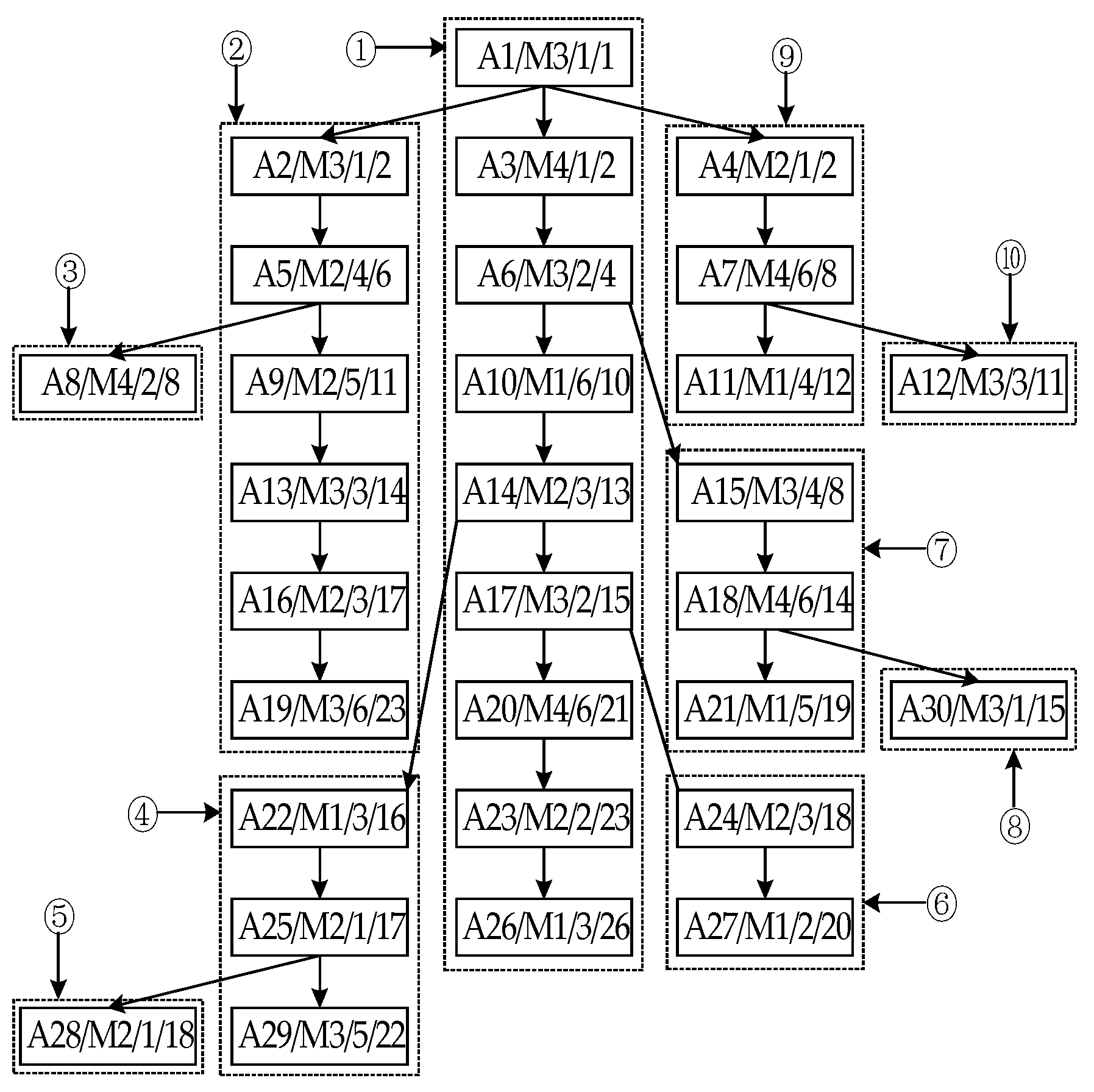
3.1.1. Case

Suppose that the single order product A of the manufacturing enterprise consists of 30 processes and needs to be machined on four pieces of equipment. The ROPT of product A is shown in Figure 1. The unit of machining time is h. The rectangular box in ROPT represents the process. The information in the rectangular box is the four attributes of the process: process name/equipment name/machining time/PLoN.

3.1.2. Scheduling Results

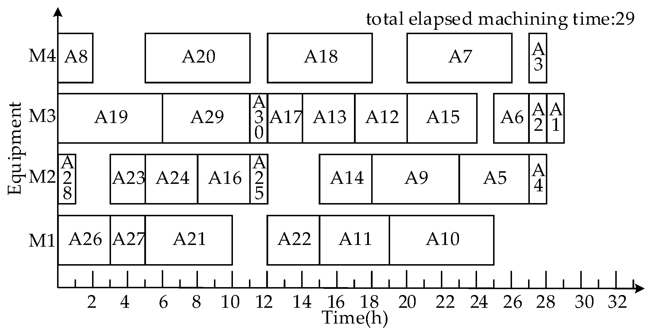
• Scheduling product A using the ROHISA

In order to facilitate readers in understanding the ROHISA, the following is a further illustration with the help of the scheduling example of product A.

(1)

Process Sorting

We apply Algorithm 1 to sort all the processes in ROPT. We describe the process of sorting the leaf nodes in the first layer from large to small according to the TUD of the PS to which they belong. The situation of other layers will not be repeated. The division diagram of PS when establishing the 1st LA is shown in Figure 2, the ROPT is divided into ten PSs, ① to ⑩.

The sorting process is briefly described as follows.

(1)

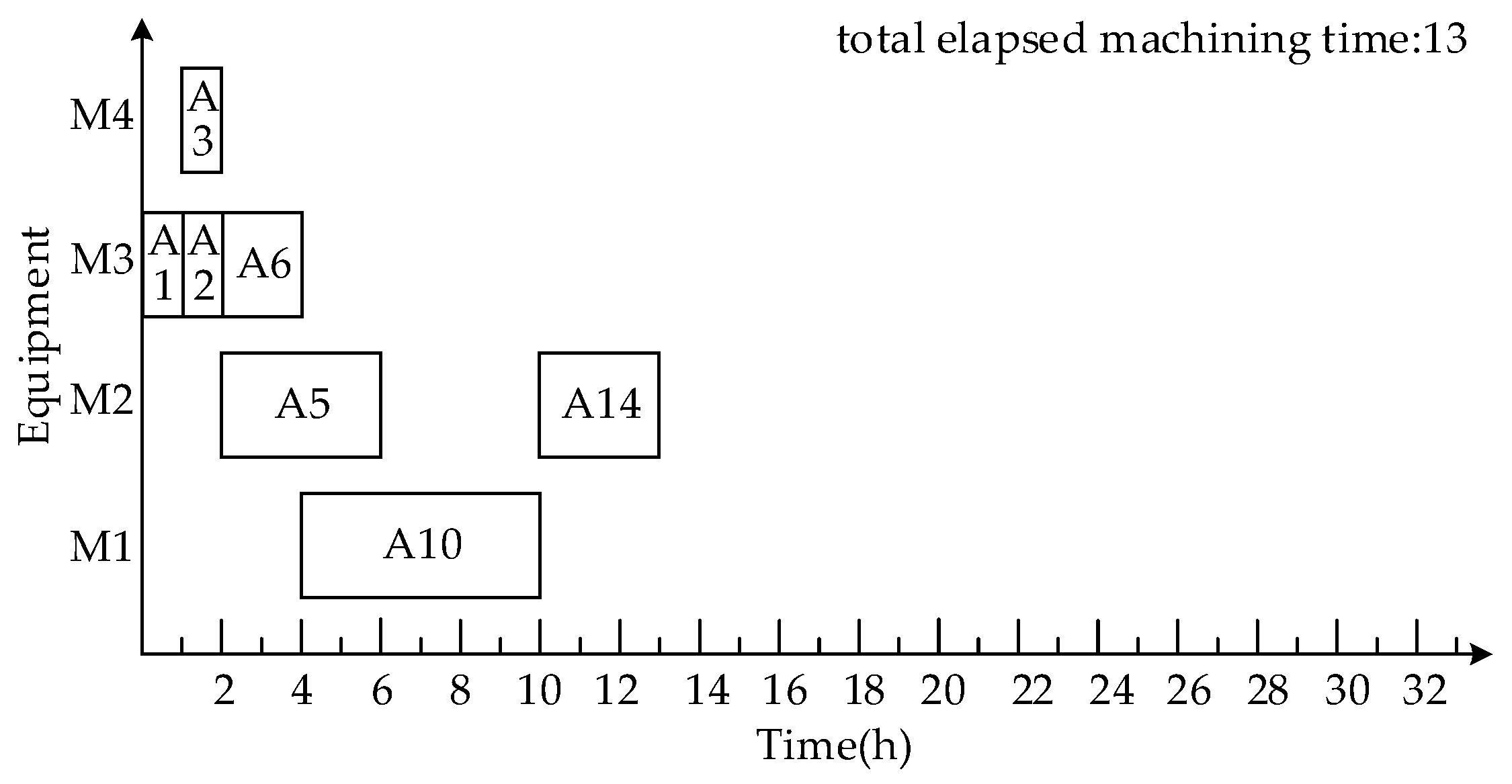
The first step

We initialize lsit0 and lsit1 to be empty and create ROPT. We calculate each PloN and the number of layers in ROPT and then obtain N = 9. Because the PloN of A26 is the longest, its value is 26 h, and we determine its PoN ① as CP. We update the value of all nodes’ attribute L. We initialize Layeri (1 ≤ i ≤ 9) and let i = 0. We use Lsit1 to back up Lsit0. Because the leaf nodes’ number is 10, which is greater than 1, Algorithm 2 is called.

(2)

The second step

Go to Algorithm 2, and the process is as follows.

Step 1. We initialize a [], b [], Stack1, Stack2 to be null. We let j = 0 and i = i + 1.

Step 2. We determine A26′s PoN ① as CP, which is the PS with the largest TUD.

Step 3. We store the CP’s last node A26 to Layer1 [0] and q₁ is the pointer pointed to the PS’s first process A1. According to the order from the root node to leaf node, we judge whether each process is a fork node. We push the fork nodes into Stack1. Therefore, the Stack1′s contents are A1, A6, A14 and A17 from bottom to top. We delete this path from the ROPT. As the elements popped out from Stack1 in turn, we obtain the five unique longest PSs, starting from their immediate successor processes, which are (A24, A27), (A22, A25, A29), (A15, A18, A21), (A4, A7, A11), (A2, A5, A9, A13, A16, A19). a [] = {⑥, ④, ⑦, ⑨, ②}. We calculate the TUD values of the five PSs and store them in b [], so b [] = {−6, −4, −7, −14, −3}. We sort the elements in a [] according to the corresponding elements’ value of b [] from small to large. When the values are equal, we sort them according to the number of processes contained in PS, from small to large. Therefore, we obtain a [] = {⑨, ⑦, ⑥, ④, ②}. We push the elements from a [] into Stack2 in order from front to back and empty a [] and b []. Therefore, the elements in Stack2 from bottom to top are ⑨, ⑦, ⑥, ④ and ②.

Step 4. Stack2 pops up. The PS ② is regarded as the PS that has the largest TUD value of its subtree, and we proceed to Step 3. We store A19 in layer1 [1] and point to A2 with the pointer q₂. Then, we push A5 into Stack1 and delete PS ② from the forest. Stack1 pops up. Then, we obtain a PS, which is A8. There is only one PS, so a [] = {③}. We push ③ into Stack2 and empty a [] and b []. The elements in Stack2 from bottom to top are ⑨, ⑦, ⑥, ④, ③.

Step 5. We repeat Step 4 until Stack2 is empty. Finally, we obtain the LA of the i-th layer.

Step 6. We first copy List1 with List0, delete all leaf nodes from List0, and then back up List0 with List1. For the ROPT stored by List0, we go to the second step. Layer2 [] ~ Layer9 [] are obtained by repeating the above operation process, as shown below.

Layer1 [] = [A26, A19, A8, A29, A28, A27, A21, A30, A11, A12]

Layer2 [] = [A23, A24, A16, A25, A18, A7]

Layer3 [] = [A20, A22, A13, A15, A4]

Layer4 [] = [A17, A9]

Layer5 [] = [A14, A5]

Layer6 [] = [A10, A2]

Layer7 [] = [A6]

Layer8 [] = [A3]

Layer9 [] = [A1]

(3)

The third step

We reverse the order of nine Layeri (1 ≤ i ≤ 9) and the elements’ order in each array. The results are as follows.

Layer1 [] = [A1]

Layer2 [] = [A3]

Layer3 [] = [A6]

Layer4 [] = [A2, A10]

Layer5 [] = [A5, A14]

Layer6 [] = [A9, A17]

Layer7 [] = [A4, A15, A13, A22, A20]

Layer8 [] = [A7, A18, A25, A16, A24, A23]

Layer9 [] = [A12, A11, A30, A21, A27, A28, A29, A8, A19, A26]

(2)

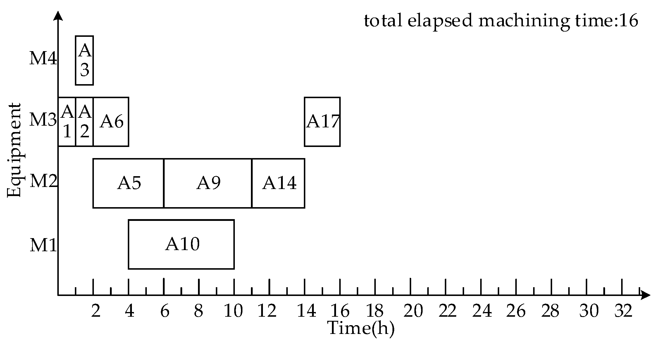
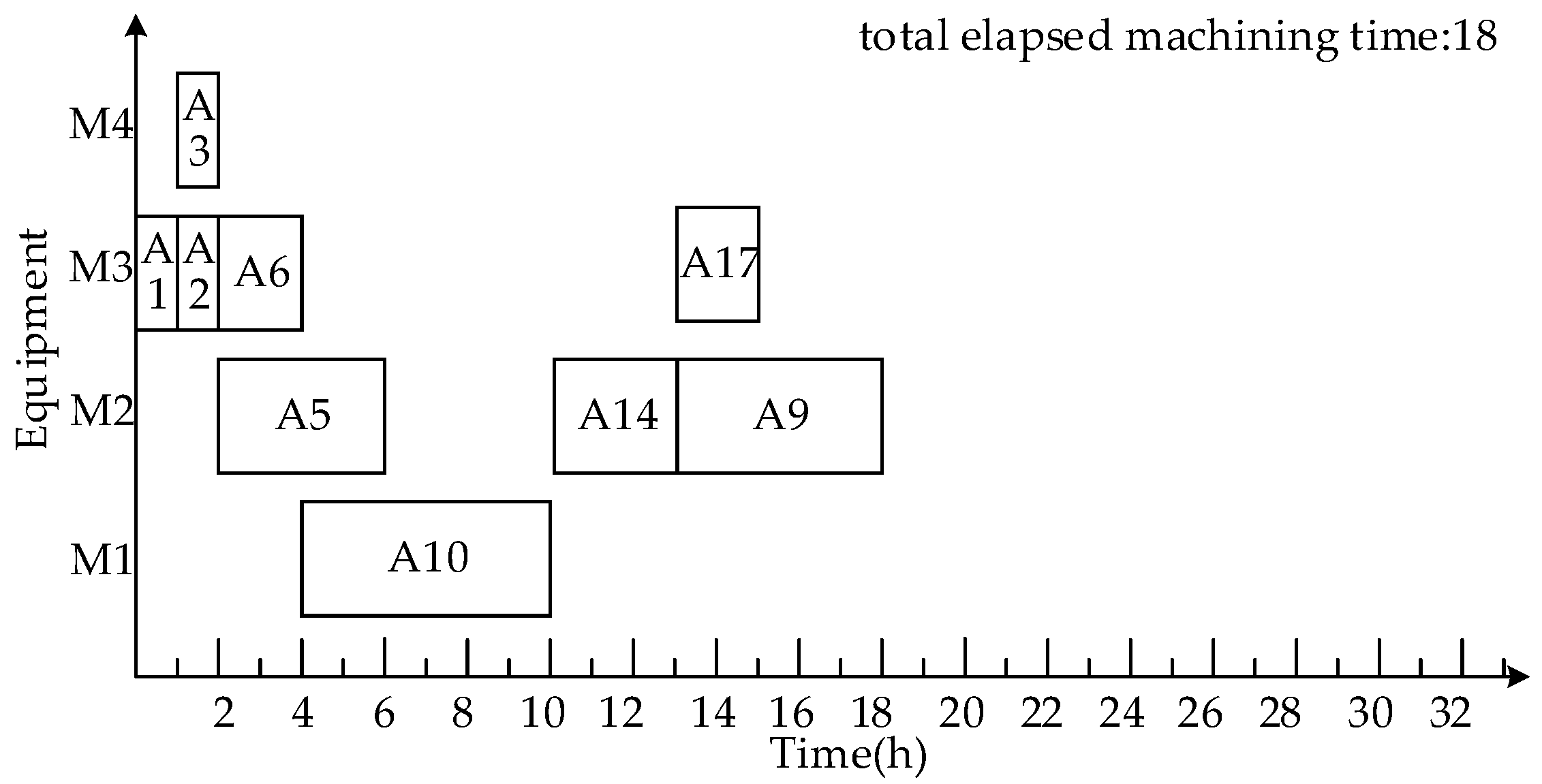
Process Scheduling

By applying the proposed Algorithm 6 to schedule the sorted Las, in turn, we obtain SS_SLP P₁~P₉, where P₉ is the PSS P. The Gantt chart of P₅ is shown in Figure 3. Next, we will briefly describe the process of establishing P₆ based on P₅, and the establishment process of other SS_SLPs will not be repeated. The processes in Layaer6 are A9 and A17. The QSTP of A9 is 6 and 13 from front to back, and the QSTP of A17 is the machining end time of A14. A9 starts machining at time point 6, and the Gantt chart of QSS_SLP P₆¹ is shown in Figure 4. A9 starts machining at time point 13, and the Gantt chart of QSS_SLP P₆² is shown in Figure 5. We select P₆¹ with the minimal ET_QSS as the SS_SLP P₆. The Gantt chart of scheduling product A using the ROHISA is shown in Figure 6, and the product manufacturing makespan is 28 h.

2.

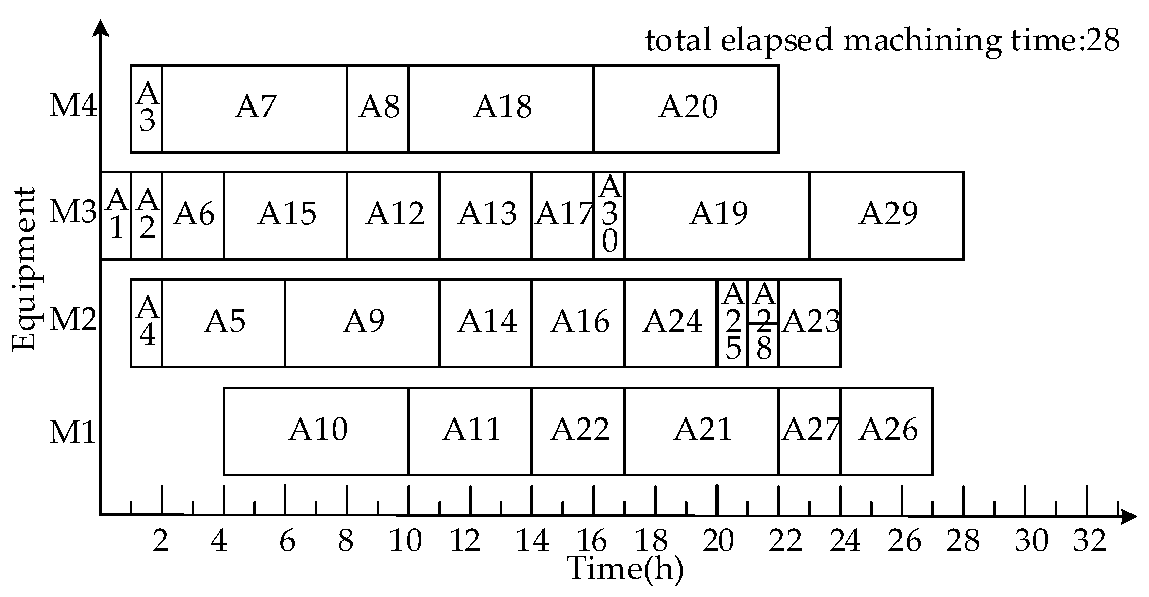
Scheduling product A using a time-selective integrated scheduling algorithm (TISA)

The PS sorting strategy sorts the 10 PS_S of A as follows: A1→A26, A2→A19, A15→A21, A4→A11, A22→A29, A24→A27, A12, A8, A28, A30. According to the TISA proposed in reference [18], in the scheduling process, based on the initial SS formed by CP A1->A26, we obtain a set of quasi-scheduling schemes aimed at each process’s trial scheduling. We select the current optimal SS from the set as the final SS of the process. The Gantt chart of scheduling A using TISA is shown in Figure 7. The manufacturing makespan of product A is 32 h.

3.

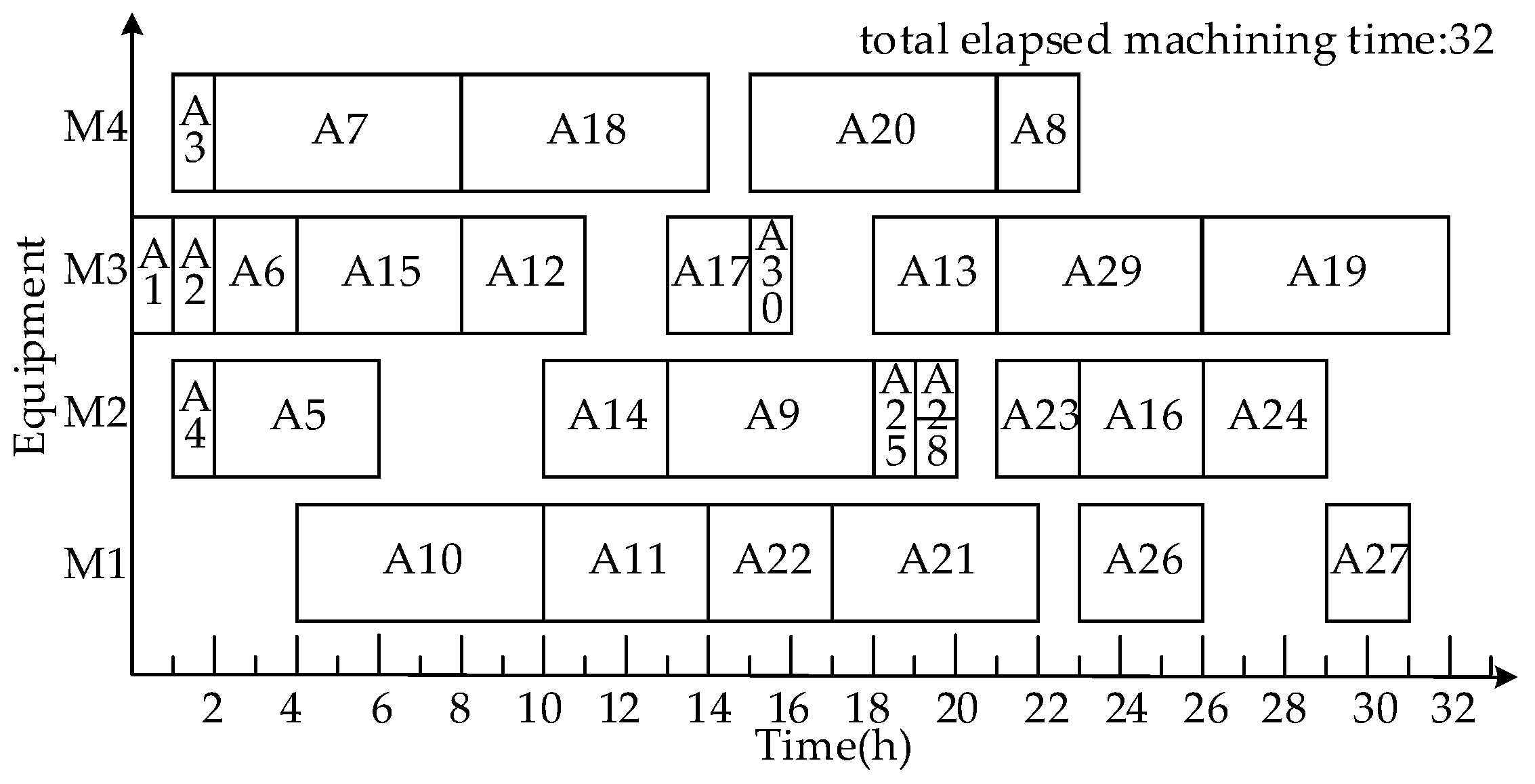
Scheduling product A using the dynamic critical paths method (DCPM)

Dynamic CP strategy and short time strategy sort all processes of A as follows: A26, A23, A19, A29, A20, A27, A21, A28, A24, A25, A16, A22, A30, A17, A13, A18, A14, A11, A12, A9, A10, A8, A15, A7, A5, A6, A2, A3, A4, A1. According to the DCPM proposed in reference [23], the first adaptive scheduling strategy is adopted. The Gantt chart of scheduling product A using DCPM is shown in Figure 8. The manufacturing makespan of product A is 29 h.

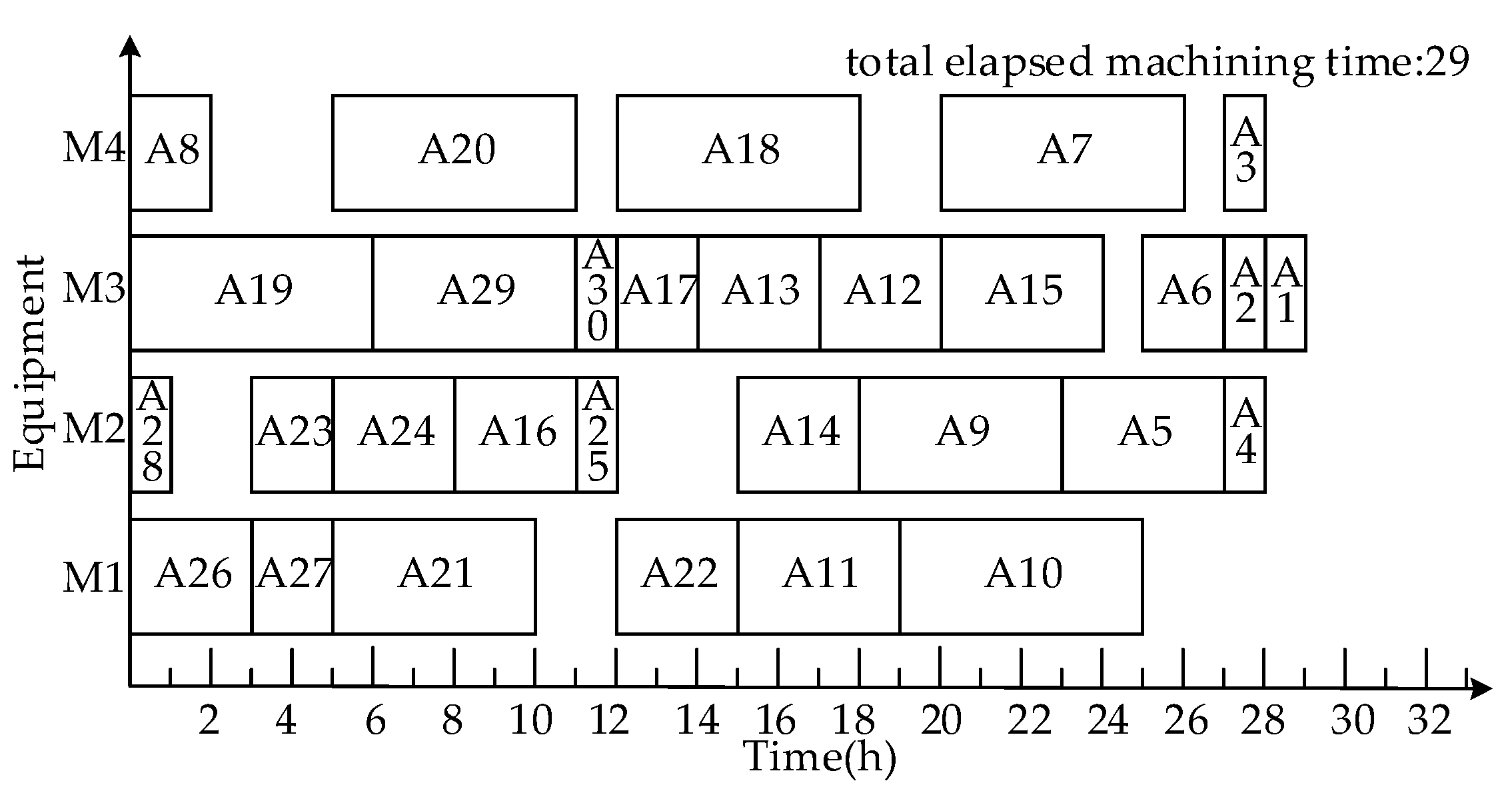
4.

Scheduling product A using a machine-driven integrated scheduling algorithm with rollback-preemptive (MISAR)

According to the MISAR proposed in reference [22], the maximum parallelism selection strategy is adopted. The Gantt chart of scheduling A using MISAR is shown in Figure 9. The manufacturing makespan of product A is 29 h.

3.1.3. Comparison and Analysis

For the integrated scheduling of product A, we find that the ROHISA is the best, MISAR and DCPM are the second best, and TISA is the worst by comparing Figure 6 and Figure 9. The completion time of the ROHISA is 12.5% shorter than that of TISA.

TISA is easy to make the scheduling result fall into local optimization. For example, when scheduling A9, the three QSTPs of A9 are 6, 13 and 23, respectively. TISA selects QSTP 13 to schedule A9. At present, although this SS takes the least time, it not only causes the idle time between A5 and A14 on M2 but also delays the completion time of PS where A9 is located, resulting in poor product scheduling results.

DCPM gives priority to A19, resulting in poor product scheduling results. A19 and A29 need the same equipment, and their PloN is 23 and 22 h, respectively. The TUD value of PS A2->A19 is 23−26 = −3, which is larger than that of PS A22->A29, which is 22−26 = −4. According to the definition of TUD, the smaller the machining completion time of PS A2->A19, the smaller the product completion time. The completion time of A2->A19 using DCPM is 28 h, while the completion time of A2->A19 using the ROHISA is 22 h.

MISAR’s poor scheduling result is the same as using DCPM. For example, when we use the maximum parallelism selection strategy to select the process for M3, A19 and A29 have the same parent node PloN. At the same time, the machining time of A19 is greater than that of A29. MISAR gives priority to allocating M3 for A19, resulting in poor product scheduling results.

3.2. Experimental Data Comparison and Analysis

3.2.1. Experimental Data and Environment

Without losing generality, 100 product PTs were randomly generated. The following parameters were randomly generated: the number of processes is [20,50], the number of immediate predecessor processes of each non-leaf node is [1,10], the number of machining equipment is [3,10], and the machining time of a process is [1,20]. The software used on the experimental platform was Windows 7, 64-bit, GCC5.0, and the hardware of the experimental platform was an Intel Core i5-3470S processor with 4 GB of memory.

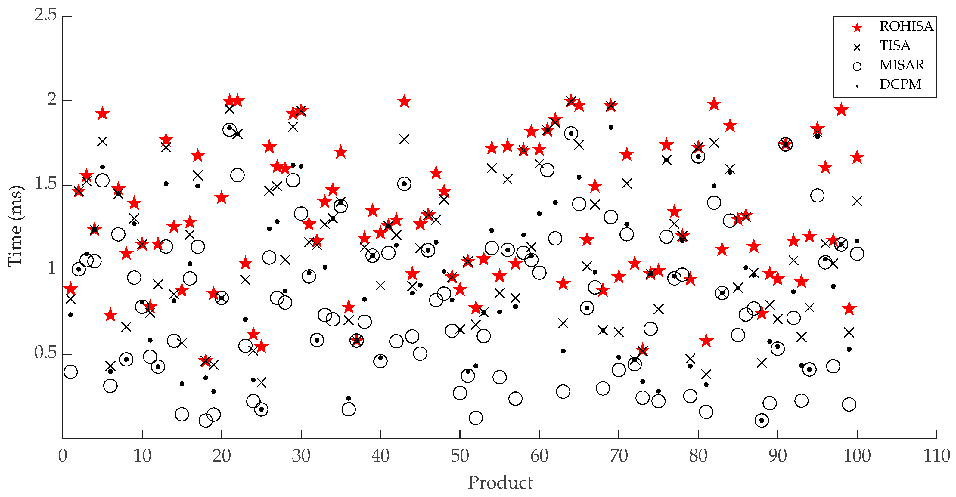
3.2.2. Statistical Comparison of Experimental Results

Experiments were designed as follows: comparison of the results of scheduling 100 trees by the TISA, DCPM, MISAR, and ROHISA (Figure 10), comparison of the execution time to schedule 100 trees by the four algorithms (Figure 11), and comparison of the average machining and execution time to schedule 100 trees by the four algorithms (

Table 1. Average machining time and execution time to schedule 100 trees by the four algorithms.

Algorithm	Average Machining Time (h)	Average Execution Time (ms)
TISA	744.3	1.143456
DCPM	734.77	0.967637
MISAR	726.43	0.799919
ROHISA	717.57	1.314644

).

3.2.3. Analysis of Experimental Results

In Figure 10, the x-axis represents 100 trees, and the y-axis represents the total elapsed machining time. Because the optimization goal of the integrated scheduling problem is to minimize the total product machining completion time, the closer to the x-axis we are, the better the scheduling results we obtain. It can be seen from Figure 10 that the scheduling results of the ROHISA are generally better than those of the TISA, DCPM, and MISAR. This is also illustrated by the average data in Table 1. Figure 11 and Table 1 indicate that the execution time of ROHISA is slightly higher than that of the other three algorithms.

4. Discussion

We compared our ROHISA with the current advanced TISA, DCPM, and MISAR. The results indicate that our algorithm outperforms them. The ROHISA does take longer to execute; however, with the rapid development of computer hardware, algorithm designers generally aim to achieve better results by sacrificing minor computer resources.

5. Conclusions

The ROHISA proposed in this paper takes one layer of processes as a unit for trial scheduling and gives priority to the process on PS, which has a great impact on the product manufacturing makespan and overcomes the disadvantage of easily falling into a local optimal when taking a single process as a unit. Therefore, it optimizes the general integrated scheduling results for single-product manufacturing enterprises and improves production efficiency.

Although the time complexity of the ROHISA is no more than cubic polynomial, through experimental data comparison and analysis, it has been proven that its executing time is slightly greater than those of TISA, DCPM and MISAR, but its total elapsed machining time is generally less. It is in line with the goal of single-product manufacturing enterprises and researchers to exchange a small amount of time for good scheduling results.

This research fills the gap in the literature on the TUD of PS. The research results can be applied to the production activities of single-product manufacturing enterprises. The engineering and scientific problems analyzed and refined in the research process will have common characteristics for ‘Internet + Intelligent Manufacturing’ and promote the implementation of ‘Made in China 2025′.

In the future, the research on the dynamic TUD of all schedulable processes in the current PT will promote the development of integrated scheduling.

References

- Hua, H.M. Subversion of the Global Manufacturing Industrie 4.0, 1st ed.; Publishing House of Electronics Industry: Beijing, China, 2015; pp. 10–14. [Google Scholar]
- Nica, E.; Stan, C.I.; Luțan, A.G.; Oașa, R.-Ș. Internet of Things-based Real-Time Production Logistics, Sustainable Industrial Value Creation, and Artificial Intelligence-driven Big Data Analytics in Cyber-Physical Smart Manufacturing Systems. Econ. Manag. Financ. Mark. 2021, 16, 52–62. [Google Scholar] [CrossRef]
- Lăzăroiu, G.; Kliestik, T.; Novak, A. Internet of Things Smart Devices, Industrial Artificial Intelligence, and Real-Time Sensor Networks in Sustainable Cyber-Physical Production Systems. J. Self-Gov. Manag. Econ. 2021, 9, 20–30. [Google Scholar] [CrossRef]
- Yin, J. Resource Scheduling Optimization and Engineering Application, 1st ed.; Metallurgical Industry Press: Beijing, China, 2018; pp. 23–31. [Google Scholar]
- Zhang, F.F.; Mei, Y.; Nguyen, S.; Zhang, M.J. Collaborative Multifidelity-Based Surrogate Models for Genetic Programming in Dynamic Flexible Job Shop Scheduling. IEEE Trans. Cybern. 2021, 99, 1–15. [Google Scholar] [CrossRef] [PubMed]
- Pei, Z.; Zhang, X.F.; Zheng, L.; Wan, M.Z. A column generation-based approach for proportionate flexible two-stage no-wait job shop scheduling. Int. J. Prod. Res. 2020, 58, 487–508. [Google Scholar] [CrossRef]
- Li, X.P.; Yu, W.; Ruiz, R.B.; Zhu, J. Energy-aware cloud workflow applications scheduling with geo-distributed data. IEEE Trans. Serv. Comput. 2022, 15, 891–903. [Google Scholar] [CrossRef]
- Li, X.P.; Chen, F.C.; Ruiz, R.B.; Zhu, J. MapReduce task scheduling in heterogeneous geo-distributed data centers. IEEE Trans. Serv. Comput. 2021, 99, 1. [Google Scholar] [CrossRef]
- Guo, S.P.; Dong, M. Order matching mechanism of the production intermediation internet platform between retailers and manufacturers. Int. J. Adv. Manuf. Technol. 2020, 115, 949–962. [Google Scholar] [CrossRef]
- Zou, W.Q.; Pan, Q.K.; Wang, L. An effective multi-objective evolutionary algorithm for solving the AGV scheduling problem with pickup and delivery. Knowl.-Based Syst. 2021, 218, 106881. [Google Scholar] [CrossRef]
- Chang, X.F. Challenges Posed by Multi Variety and Small Batch Production Mode and Countermeasures Acted by Chinese Small and Medium Enterprises. Adv. Mater. Res. 2013, 2393, 794–798. [Google Scholar] [CrossRef]
- Xie, Z.Q.; Yang, D.; Ma, M.R.; Yu, X. An Improved Artificial Bee Colony Algorithm for the Flexible Integrated Scheduling Problem Using Networked Devices Collaboration. Int. J. Coop. Inf. Syst. 2020, 29, 2040003. [Google Scholar] [CrossRef]
- Gao, Y.L.; Xie, Z.Q.; Yang, D.; Yu, X. Flexible integrated scheduling algorithm based on remaining work probability selection coding. Expert Syst. 2021, 38, e12683. [Google Scholar] [CrossRef]
- Xu, X.L.; Li, L.; Fan, L.X.; Zhang, J.; Yang, X.H.; Wang, W.L. Hybrid Discrete Differential Evolution Algorithm for Lot Splitting with Capacity Constraints in Flexible Job Scheduling. Math. Probl Eng. 2013, 2013, 112–128. [Google Scholar] [CrossRef]
- Novak, A.; Bennett, D.; Kliestik, T. Product Decision-Making Information Systems, Real-Time Sensor Networks, and Artificial Intelligence-driven Big Data Analytics in Sustainable Industry 4.0. Econ. Manag. Financ. Mark. 2021, 16, 62–72. [Google Scholar] [CrossRef]
- Nica, E.; Stehel, V. Internet of Things Sensing Networks, Artificial Intelligence-based Decision-Making Algorithms, and Real-Time Process Monitoring in Sustainable Industry 4.0. J. Self-Gov. Manag. Econ. 2021, 9, 35–47. [Google Scholar] [CrossRef]
- Liu, D.J.; Hu, C.M. A dynamic critical path method for project scheduling based on a generalised fuzzy similarity. J. Oper. Res. Soc. 2021, 72, 458–470. [Google Scholar] [CrossRef]
- Xie, Z.Q.; Zhang, X.H.; Gao, Y.L.; Xin, Y. Time-selective Integrated Scheduling Algorithm Considering the Compactness of Serial Processes. Chin. J. Mech. Eng. 2018, 54, 191–202. [Google Scholar] [CrossRef]
- Zhang, X.H.; Ma, C.; Wu, J. Multi-batch integrated scheduling algorithm based on time-selective. Multimed Tools Appl. 2019, 78, 29989–30010. [Google Scholar] [CrossRef]
- Wang, Z.; Zhang, X.H.; Peng, G. An Improved Integrated Scheduling Algorithm with Process Sequence Time-Selective Strategy. Complexity 2021, 2021, 5570575. [Google Scholar] [CrossRef]
- Cao, W.C.; Xie, Z.Q.; Pei, L.R. Reverse Order and Greedy Integrated Scheduling Algorithm Considering Dynamic TUD of the Process Sequences. J. Electron. Inf. Technol. 2022, 44, 1572–1580. [Google Scholar] [CrossRef]
- Xie, Z.Q.; Xin, Y.; Yang, J. Machine-driven integrated scheduling algorithm with rollback-preemptive. Acta Autom. Sin. 2011, 37, 1332–1343. [Google Scholar] [CrossRef]
- Xie, Z.Q.; Yang, J.; Zhou, Y.; Zhang, D.L.; Tan, G.Y. Dynamic critical paths multi-product manufacturing scheduling algorithm based on operation set. Chin. J. Comput. 2011, 34, 406–412. [Google Scholar] [CrossRef]