1. Introduction
The high-speed train (HST) has become the most prominent mode of transport for passengers, especially in densely populated countries. Additionally, wireless channel modeling for HSTs has become a growing study area [
1]. Apart from handling critical signaling, the HST communication system in 5G and beyond is expected to provide a variety of stable onboard broadband services such as the Internet of Things for the railway, real-time train dispatch, onboard internet access, etc. However, present technologies allow data rate transmission of up to a maximum of 100 Mbps [
2,
3]. This can only be accommodated in the interconnection required for the future HST communication infrastructure [
4].
Implementing millimeter wave (mmWave) technologies for future rail communication services is a viable strategy for achieving the required data-rates for 5G transmission and beyond [
2,
5,
6]. This has been seen in the development of a mmWave-based mobile hotspot network (MHN) structure in [
7]. In this system, the field trials and simulations have shown that a throughput of 7 Gbps can be achieved in the downlink when the train speed is 500 km/h. The single-frequency multi-flow (SFMF) transmission technique was used to achieve this peak throughput. In addition, mmWAve band measurements between the train and truck were carried out by [
8] at 41 GHz. The channel characteristics like the LCR and average fading duration were investigated thoroughly when the velocity between the receiver and transmitter was 170 km/h. In addition the research on measurement done in [
7,
8], simulations of wireless channel models have also been done in [
9,
10,
11]. A GBSM approach for mmWave bands was introduced in [
9], although this was based on ray tracer simulation. In the work of [
11], the channel characteristics of HST environments, such as tunnels and urban environments, were analyzed using ray tracing at 30 GHz. Most of the channel statistics in these environments have been studied using ray tracing, which also has a shortcoming of computational complexity when compared to geometry-based stochastic models (GBSM).
Although these studies have been carried out, the implementation of the mmWave band for HST communications in environments like cutting and viaducts continues to face different challenges. One of the challenges is the lack of channel models, especially geometry-based stochastic models, which can mimic the channel environments. The available models have focused on the lower sub-band of 5G, such as in [
12,
13]. Results from these models cannot be just extended to mmWave bands without addressing the shortcoming of scatterers, which could be captured using 3D geometry. In addition, some channel models like the IMT-A channel model have not introduced the other high-speed train channel environments, like viaducts and cutting, whereas the impact of breaking distance has not been considered in these channel environments [
14]. Thus, with this motivation, a non-stationary 3D GBSM MIMO for viaduct and cutting environments for the 5G channel was proposed. Since coverage is important for mmWave band channels, when modeling a channel, it is important to consider the 3D (elevation angles) and the MIMO. Incorporating the two enables the proposed channel models to be extended to massive MIMO with different planes, such as cylindrical or spherical, to enhance coverage for mmWave channels. Elevation angles are also important in the cutting environment when directional antennas are used and the mobile radio station (MRS) is very close to the base station (BS).
In this paper, a generic model is proposed that is an extension of the one in [
15], which was considered for this open-case scenario. A GBSM consists of one sphere and many confocal elliptic cylinders representing the stationary and uniformly distributed scatterers and the non-stationary environment situations, respectively. A time-variant Rician K-factor was introduced in the viaduct and cutting scenarios. This is important due to the effect of dimension structure in these two environments. The derived LCR of the proposed model is used to characterize the fast-changing nature of the channel at mmWave frequency and also compare it with lower-band carrier frequency channels.
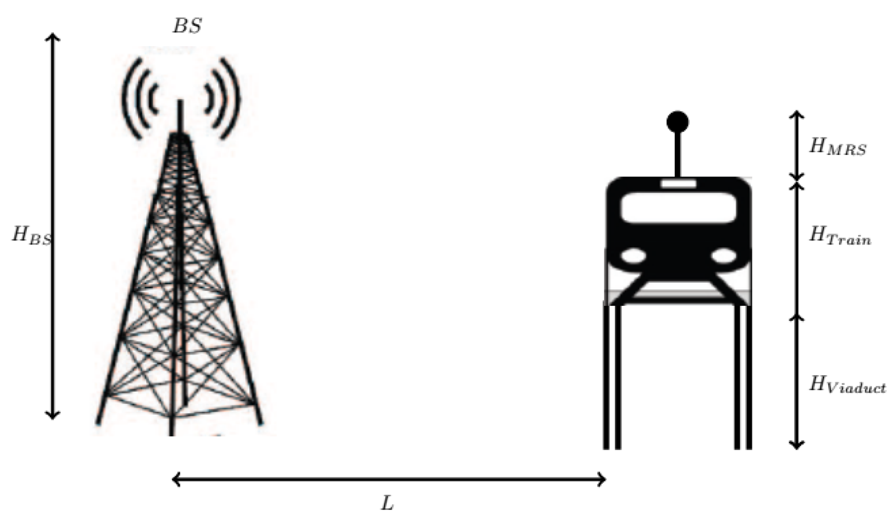
1.1. The Viaduct Environment
Some of the parameters that influence the wireless channel of the viaduct environment have been illustrated in
Figure 1. Viaducts usually cover over
of the HST mileage [
16]. Viaducts enable a connection of two points of terrain that appear to be of the same height. On the other hand, these can also be used to pass over water, a valley, or a road. Viaducts provide smooth rails to enhance the higher speed of the train. In the viaduct environment, the multipath components are associated with reflection or scattering from obstacles like tall buildings or trees. The relative height between the BS and the viaduct strongly impacts the received signal. The LOS component is dominating in this situation due to the viaduct’s relatively high altitude to the surrounding topography. However, the distribution of the surrounding scatterers still impacts the received signal.
1.2. The Cutting Environment
The cutting environment is common in an HST’s mileage, and the parameters that influence the wireless channel of the cutting environment have been illustrated in
Figure 2. During construction of the HST track on uneven terrain like hills, a cutting environment is utilized to enable the train to traverse through the large obstacles. This guarantees that the tracks are flat and that the train travels at a fast speed. In the case where the steep sidewalls of the track have approximately the same depth, this is commonly known as regular cutting. Regular cutting is the most common cutting used. Although the received signal will have a strong LOS component, the steep walls may result in multiple reflections and scattering components. The crown width and bottom width of cuttings are considered in the analysis of channel statistics.
2. The Proposed Non-Stationary Model for High-Speed Train mmWave Band Channel
We consider the architecture which consists of a mobile relay station on the vehicle and the base station on the side of the track. The two stations for outdoor communication consists of MIMO antennas with S receive and U transit antenna elements, respectively. The BS and MRS are separated by a time-varying distance of
. The GBSM suggested in [
15] as shown in
Figure 3 is made up of components from the line of sight, the single bounce from the sphere, and the multiple confocal rays from the elliptic cylinder. The model consists of a sphere and an elliptic cylinder representing the environment scatterers. We adopt a
MIMO channel model as an illustration for clarification as an example. The proposed 3D model could be extended to a massive MIMO in a different plane.
The first and other taps are represented using the tapped delay line (TDL) Structure. For the first tap, we suppose that around the sphere with radius , the receiver is located in the center. There are scatterers on the sphere, whereas an effective scatterer is defined by . The elliptic cylinder is represented by the multiple confocal elliptic-cylinder models using a time delay line structure.The transmitter Bs and the receiver MRs are located at the two foci, respectively.The scatterers are located on the elliptic-cylinder, where . represents the time-variant total number of taps. The scatterer on the semi major axis of the elliptic cylinder is defined by . The time-varying semi-minor axis of the lth tap (elliptic cylinder) is denoted by . In this case, the half length between the two foci is represented by , which is also equal to . The MRs and the BS have been tilted at an angle and , whereas the elevation of the antenna array is represented by and , respectively.The moving direction and the velocity of the MRs denoted by and respectively. The elevation angle of arrival and the azimuth angle of arrival of the LOS component are represented by and , respectively. The azimuth angle of departure and elevation angle of departure are denoted by and , respectively.
Based on [
12], the channel impulse response
where the complex space-time-variant tap coefficients
and discrete propagation delay
of the
lth tap have been represented. This is obtained from the superposition of the components from the LoS, sphere and the elliptic cylinder. The multipath components from the sphere and elliptic cylinder are also known as single bounce components (SB) represented by
, where
i is the component from either the sphere
or from the elliptic cylinder
.
The spacing of the transmitter (Tx) and receiver (Rx) antenna elements are denoted by
and
, respectively. The half length distance between the foci of the ellipse is denoted by
f. Therefore,
represents the distance
D between the Tx and Rx. In this theoretical model, some assumptions, such as min
max
,
and
, have been used. From Equation (
1), the first tap consists of the LOS component and the summation of the single-bounce component from the sphere and the first single-bounce component from the elliptic cylinder. Therefore, from the equation
where
The parameters and are time varying. This makes the underlying GBSM a non-stationary one. designates the mean power for the tap, , and links and , respectively. The k and c represent the Rician K-factor and speed of light, respectively. The parameters related to energy are , which define the percentage contribution of single-bouncing rays to the overall scattered power of the first tap. It is worth noting that these energy-related characteristics have been standardized to meet the requirements .
For other taps, the complex tap coefficients
of only SB components make up the link
. The other taps consist of the single-bounce component from the elliptic cylinder, which is also the multiple confocal elliptic cylinder. This may be written as
where
is the time it takes for waves to travel via the link
. For other taps, parameters related to power are
which define the percentage contribution of single-bouncing rays to the overall scattered power of the other taps, and it satisfies
. The phases
and
i.i.d. are random variables that are uniformly distributed over
, while the maximum Doppler frequency relative to the mobile station is denoted by
.
In the case of the first tap, SB rays are generated from the scatterers on either the sphere or the first elliptic cylinder on addition to the los component, as shown in
Figure 3. For additional taps, the SB rays components are assumed to be generated from the scatterers located on the corresponding elliptic cylinder. The underlying assumptions as in [
17] are based on the application of the cosine laws in triangles (i.e.,
and
for small
x). Deducing min
max
,
and
, we have
where
,
,
,
,
,
,
, and
with
denoting the semi-minor axis of the
elliptic-cylinder. The azimuth angle of departure (AAoD)/elevation angle of departure (EAoD) (i.e.,
) and azimuth angle of arriva (AAoA)/elevation angle of arrival (EAoA) (i.e.,
) for the SB rays are correlated. From the sphere model, the derivation of the relationship between angle of arrival (AoA) and the angle of departure (AoD) SB components are:
,
. The angular relationships for SB rays derived from the elliptic cylinder model are:
, and
hold with
, denoting the semi axis of the
elliptic cylinder. The discrete AAoD is used in the proposed theoretical 3D GBSM as the number of scatterers approaches infinity.
, EAoD
, AAoA
and EAoA
can be replaced by continuous random variables
,
,
and
, respectively, to consider the effects of azimuth and elevation angles on channel statistics simultaneously. In addition, to characterize the distribution of effective scatterers, we employ the von Mises–Fisher (VMF) probability density function (PDF), which was described in [
17], since a 3D GBSM model was also applied.
where
,
,
account for the mean values of the azimuth angle
and the elevation angle
, respectively, and
is a real valued parameter that controls the concentration of the distribution as identified by the mean direction
and
. In this case, for angular descriptions, i.e., the AAoA
and EAoA
for the sphere and the AAoA
and EAoA
for the multiple elliptic cylinders, the parameters
and
k) of the VMF PDF are in
and
and
and
, respectively. By considering the scenario of the line of sight (LoS) component, the time varying AAoA
and EAoA
can be expressed as
where
denotes the initial LoS AOA at time
.
By considering the scenario of a single-bounce
component resulting from the Rx sphere, the time-varying AAoD
EAoD
, and AAoA
and EAoA
can be expressed as
By considering the scenario of the single-bounce components
representing the
tap resulting from the elliptic cylinder, time-varying AAoA
and EAoA
can be expressed as
The time-varying AAoD
and EAoD
can be noted as correlated signals with the time varying AAoA
and EAoA
for SB rays resulting from the elliptic cylinder model. Therefore, the relationship between the AoA and AoD for multiple confocal elliptic cylinder models can be given by
2.1. Viaducts and the Time-Varying Rician K-Parameters
The main attributes of the viaduct structure that affect the received signal by the MRS are shown in
Figure 1. The sectional view of the viaduct scenario shows that the MRS is installed on top of the train. The significance of the viaduct structure’s attributes, particularly the viaduct’s height,
, and the distance between BS and MRS have been used to study the impact of the time-varying Rician K-factor, and the equation is obtained from [
18]. In this case,
, whereas the minimum distance can be calculated as
. The Rician K-factor,
, in the viaduct scenario can be expressed as
2.2. Cutting and the Time Varying Rician K-Parameter
Figure 2 shows a sectional illustration of the cutting scenario with the critical variables of the cutting construction. The sidewalls in the cutting have a significant impact on the received signal. Cutting is classified in two scenarios: deep cutting
and low cutting
scenarios. The dimension structures of
and
are represented, and the time-varying distances between the MRS and BS and the breaking point distance (
) greatly impact the Rician K-factor of the cutting environment. This is expressed as in [
19] using the following equation:
The relationship between the height of BS and MRS can be expressed as , while .
4. Numerical Analysis of the Viaduct and Cutting
For both the viaduct and cutting environments, the common parameters for all the scenarios are
km/h and
GHz. The Doppler frequency will be obtained using the formula
with respect to the
, and the MRS antenna is assumed to be placed at the rooftop of the train. The number of effective scatterers
,
. The angle parameter is
, while for the first and second tap, the angle parameters are
,
and
,
. The structural parameters used from [
18,
19] of scenario 1 were considered to obtain the k-factor for the evaluation of stationarity in both the viaduct and cutting environment, respectively, as seen in
Table 1 and
Table 2. From the measurements,
m,
m,
m,
cm,
m,
m,
m,
m and
. The viaduct parameters related to power, which are
and
, are
and
for the first and second tap, respectively. With respect to the structural dimension parameters of
H and
h, the viaduct environment will be categorized into three scenarios. For a cutting environment, the parameters used from the measurement of [
19] are
m,
m,
m,
cm, and
m. With respect to the structural dimension parameters of
and
, the cutting environment will be categorized into three scenarios. By using these parameters in the formula
m, the radius of the cell will be obtained. Here,
m,
m, and
. The parameters related to power are
and
, which are
and
for the first and second tap, respectively.
Figure 4 shows how stationarity distance is affected at mmWave frequencies in the two environments when the proposed model is used. These results have been compared with the measurement campaign in [
22] for ITU. The parameters used for the viaduct environment were
km/h,
m,
m,
m,
cm, and
m whereas for the cutting environment, the parameters used were
km/h,
m,
m,
m,
cm,
m,
m, and
m. The average stationary interval for the cutting environment obtained was
m, while the average stationary interval for the viaduct was
m. If compared with the stationary interval range(2.8 m–4.2 m) as reported in [
22], the values obtained match within the range.
The absolute values of the time-variant autocorrelation function of the proposed model for the cutting environment are shown in
Figure 5. In this case, the effect of the breakpoint distance is evaluated by considering the two scenarios. The time autocorrelation function of
is lesser than
because, apart from the structural parameters of the cutting when the MS is very close to the BS, there is a shadowing effect which causes the direct ray from the directional antenna to be very weak, thus resulting in a small k-factor value. This can be related to Equation (3). The results are based on the cutting dimension measurements made in [
19]. In this case, only 2 scenarios are considered, where cutting in scenario 2 has a wider dimension than cutting in scenario 1. This is further reflected in the results where scenario 2 has a higher correlation than scenario 1. This is due to the higher Rician k value from a stronger line-of-sight component.
Figure 6 depicts the time-variant autocorrelation function of the cutting by comparing the three scenarios. Scenario 1 has the highest value, followed by scenario 3; scenario 2 demonstrates the lowest value. In the three scenarios, it is observed that the autocorrelation function increases with the structural parameters of
. This is because the higher the value of
, the higher the Rician k-factor. Thus, a higher
is important for stronger LOS components. Therefore, the proposed model can capture the channel statistics of the Rician k-factor.
From the three scenarios in
Figure 7, it is observed that varying
H of the viaduct affects the Rician k-factor value. This concerns the height of the scatterers around the viaduct, which was highlighted in the measurements. Therefore, high values of
H give stronger LOS and thus higher ACF.
Figure 8 shows how the proposed model at mmWave frequency is compared with the lower-band carrier frequency. The highest LCR value at the threshold are obtained at the mmWave band frequency. The measured values from [
18,
19] are than those measured in [
8] at the threshold value of 0. This shows that the LCR is affected by the carrier frequency. The signal at a highercarrier frequency crosses at higer rate than at a lower freqencies, thus resulting in the higher quality of the received signal.
Figure 9 shows the proposed simulation model. This is compared with the measured results in [
8]. The simulation model approximates the measure where the highest value at a threshold is almost one. Thus, the proposed model can be used for channel modeling at mmWave frequencies.


