Abstract
The emergence of the new generation video coding standard, Versatile Video Coding (VVC), has brought along novel features rendering the new standard more efficient and flexible than its predecessors. Aside from efficient compression of 8 k or higher camera-captured content, VVC also supports a wide range of applications, including computer-generated content, high dynamic range (HDR) content, multilayer and multi-view coding, video region extraction, as well as 360° video. One of the newly introduced coding tools in VVC, offering extraction and independent coding of rectangular sub-areas within a frame, is called Subpicture. In this work, we turn our attention to frame partitioning using Subpictures in VVC, and more particularly, a content-aware partitioning is considered. To achieve that, we make use of image segmentation algorithms and properly modify them to operate on a per Coding Tree Unit (CTU) basis in order to render them compliant with the standard’s restrictions. Additionally, since subpicture boundaries need to comply with slice boundaries, we propose two methods for properly partitioning a frame using tiles/slices aiming to avoid over-partitioning of a frame. The proposed algorithms are evaluated regarding both compression efficiency and image segmentation effectiveness. Our evaluation results indicate that the proposed partitioning schemes have a negligible impact on compression efficiency and video quality
1. Introduction
In recent years, the unceasing evolution of video resolution coupled with the profound video sharing activity on the internet gave rise to the advent of new video coding standards in order to contend with the need for higher compression rates. In this regard, VCEG (Video Coding Experts Groups) and MPEG (Motion Pictures Experts Group) jointly developed a new standard named Versatile Video Coding (VVC) [1,2] which was finalized in July of 2020 and was designed to achieve about 50% bit-rate reduction over its predecessor [3], High Efficiency Video Coding (HEVC) [4], for the same visual quality, while also offering a flexibility in terms of supporting an extensive number of applications. Apart from efficient compression of camera-captured high-resolution content, 8 k or higher, VVC also adopts features to efficiently support computer-generated content, high dynamic range (HDR) content, multilayer and multi-view coding, video region extraction, as well as 360° video. In order to achieve the aforementioned coding efficiency improvement, VVC incorporates advancements over pre-existing coding tools, along with novel additions [5].
One of the newly introduced coding tools in VVC is subpictures, a high-level partitioning tool, conceptually the same as Motion Constrained Tile Set (MCTS) [6] feature in HEVC but designed in a different way in order to favor coding efficiency. Both subpictures and MCTS offer the capability of independent coding as well as extraction of rectangular sub-areas within a frame. Following the pattern of tiles and slices, subpictures divide a frame into independently encodable/decodable areas consisting of a set of blocks, while a subpicture can be defined as extractable, where the dependencies between current subpicture and subpictures within the same frame or subpictures in previous frames are broken, or non-extractable. The issue that naturally rises when a frame is partitioned concerns encoding quality losses, since coding dependencies are broken in the boundaries of independently encoded/decoded blocks. In order to reduce this inherent loss of quality, it is important to take into consideration image characteristics when defining the frame partitioning into subpictures, so that similar spatial information is gathered within the same subpicture.
In this work, we focus our attention on frame segmentation into subpictures in VVC, and more specifically, a content-dependent subpicture segmentation is considered. Our target is to reduce the inherent loss of quality posed by subpictures without affecting either their philosophy or their functionality (i.e., creating independently encodable/decodable areas). In order to detect and group similar frame areas into the same subpicture, we make use of image segmentation techniques and modify them properly for keeping up with video coding standards’ restrictions. In this respect, Otsu thresholding [7] and region growing [8] image segmentation methods are utilized, due to their simplicity and effectiveness. However, image segmentation algorithms operate on a pixel level, while in the first step of the video coding process, the frame is divided into non-overlapping blocks of pixels called Coding Tree Units (CTUs), upon which the whole coding process is carried out. In this work, we propose two algorithms, Serial Region Growing and Concurrent Region Growing, that are inspired by the abovementioned image segmentation algorithms but are designed for frame partitioning in VVC.
Another restriction posed by the standard concerns the definition of subpictures, where the subpicture boundaries need to comply with slice boundaries, while slices are defined either as a subset of a tile or a collection of tiles. After detecting similar frame areas, tiles and slices need to be appropriately defined so that over partitioning of the frame is avoided. In order to tackle this issue, proper tile/slice frame partitioning algorithms, namely Tile-oriented, Slice-oriented and Adjusted Slice-oriented algorithms, are proposed. These methods aim to further reduce the coding overhead and quality loss introduced by the inclusion of the subpicture structure by offering a more flexible tile/slice partitioning. This is achieved by foregoing definitions of unnecessary tiles and utilizing the strength of the rectangular slice structure.
According to experimental evaluation, the Serial Region Growing algorithm exhibited a superior performance both in terms of segmentation fidelity (also validated by visual results) and compression efficiency. The same stands for Slice partitioning adjustments, where experimental results indicated an improvement in both quality and compression efficiency over the trivial tile partitioning approach. Finally, comparison to the baseline VVC encoder, where no frame partitioning takes place, revealed that the proposed partitioning schemes have negligible impact on compression efficiency and video quality.
The rest of this paper is organized as follows. Section 2 discusses related work on Otsu and region growing methods in image segmentation and video coding. In Section 3, a brief description of image segmentation in VVC is provided, while in Section 4, Otsu and region growing image segmentation methods are described. Section 5 presents the proposed subpicture segmentation methods, along with the proposed tile/slice partitioning schemes according to VVC video coding specification. In Section 6, metrics used for evaluating image segmentation methods that could also be used in the concept of frame partitioning in subpictures are discussed. Section 7 reports the experimental evaluation results. Finally, Section 8 concludes the paper.
2. Related Work
Due its simplicity and robustness, the Otsu thresholding method has become a widely used method in image segmentation. In the Otsu method, an appropriate threshold that maximizes between-class variance is searched and based on that threshold value, the image is segmented into foreground and background. The traditional Otsu method utilizes a one-dimensional (1D) histogram, meaning that spatial correlation of pixels is not considered, leading to poor performance in low signal-to-noise ratio images. In order to tackle this, in [9], a two-dimensional (2D) Otsu implementation was introduced, utilizing both the value of each gray pixel and the mean value of neighboring pixel values. Although the 2D Otsu method achieved a better anti-noise performance, it also introduced higher computational complexity, while using the conventional partition scheme led to a relatively poor anti-noise performance [10]. In this regard, an extensive amount of works in the literature have focused on improving the 2D Otsu method. In [11] an improved image segmentation scheme based on the Otsu method was introduced. In the proposed method, the optimal threshold value is calculated by limiting the threshold selection range and searching the minimum variance ratio. In [12], 2D histogram projection along with a fast scheme, based on the wavelet transform, for searching the extrema of the projected histogram, was proposed. In [13], a modified 2D Otsu mapped the 2D histogram pixels onto different trapezoid regions in order to narrow the threshold range. In [14], the median and average filters were used in order to smooth the image, which was used in the next step to build the 2D histogram, while the optimal threshold value was selected by performing two 1D searches on the 2D histogram. In [15], the probabilities of diagonal quadrants were calculated separately in the 2D histogram in order to reduce computational complexity.
Concerning the region-growing image segmentation technique, [16] introduced three criteria based on color homogeneity. The first criterion concerned the similarity of a pixel with its neighboring pixels, the second criterion regarded similarity of a pixel on a local and regional basis, while the third criterion considered pixel similarity when compared to the average value of the studied region. After performing region growing, the proposed method continued by merging similar regions. In [8], an image segmentation method based on seeded region growing and merging was proposed. In seeded region growing, the seed pixels are chosen based on the similarity and the Euclidean distance to their neighboring pixels, while in the merging step, small regions and regions that satisfy a homogeneity function are grouped together. In [17], an automatic seed selection algorithm was proposed for color image segmentation. To determine the initial seed points, the similarity of a pixel to its neighboring pixels was considered, while a threshold was utilized for defining the best pixel candidates using the Otsu method. Additionally, the relative distance between a candidate pixel and its eight neighbors was calculated and a threshold value was used again to choose the best candidate seed pixels. In the next step of the proposed method region, growing and region-merging is performed. In [18], an automatic image segmentation method was introduced, where for performing region growing, an improved isotropic color-edge detector was utilized to obtain the color edges and used the centroids between adjacent edge regions as initial seeds. In [19], a method that effectively predicts the direction of the region-growing process by utilizing similarity and discontinuity measures was proposed.
Image segmentation also serves as a preprocessing step and is extensively used in video coding. In [20], the Otsu method was utilized in order to determine the complexity of each largest coding unit (LCU) and reduce the number of depth levels checked during the coding unit (CU) mode decision. In [21], an optimal threshold value was determined, using the 2-D Otsu method [22], [23], to accelerate the block size decision in intra-prediction for H.264. The proposed method calculates an appropriate threshold value that is then used in order to divide an image into blocks of size 4 × 4 or 16 × 16 pixels. In [24], a modified version of Otsu thresholding was introduced to reduce the complexity of CU and prediction unit (PU) mode decision processes in 3D-HEVC. In the proposed scheme, two thresholds were determined that were further refined to divide the original depth map in a foreground, a background and a middle ground, and a fast mode decision was carried out based on CTU region classification.
Although image segmentation is broadly used in video coding, none of the existing works consider the problem of content aware subpicture partitioning in VVC. In this work, we propose two subpicture partitioning algorithms, which are based on well-known image segmentation methods, but are appropriately designed for frame partitioning in video coding. Closest to the proposed work is [17], as we also use the concept of automatic seed selection and Otsu thresholding regarding homogeneity. However, the algorithm presented in [17] could not be used as is in the context of video coding, as it works on pixel basis, whereas frame partitioning in all recent video standards is applied on a block of pixels basis. Additionally, our contribution extends to efficiently applying tile/slice partitioning, respecting the restrictions posed by the VVC standard, as described in the following sections.
3. Frame Partitioning in VVC
Like most of its predecessors, VVC adopts a block-based hybrid architecture, where inter-prediction and intra-prediction are combined with transform and entropy coding. As a first step in the encoding process, a frame is partitioned into non-overlapping blocks called Coding Tree Units (CTUs); then, the basic processing units upon the whole coding process is conducted. In VVC, the maximum size of a CTU is increased to pixels, as opposed to HEVC, where a maximum CTU size of pixels is supported. In the high level of the coding process, a set of CTUs can be grouped together to form independently encodable/decodable areas within a frame. In VVC, four high-level picture partitioning schemes are incorporated, namely slices, tiles, wavefront parallel processing (WPP) and subpictures. Slices, tiles and WPP are partitioning concepts that are also present in HEVC. In VVC, however, these concepts are adopted with some modifications. Subpictures, on the other hand, refers to a newly introduced frame partitioning scheme that, while it is conceptually the same as motion-constrained tile set (MCTS) in HEVC, has a different design, which offers a better coding efficiency capability.
3.1. Tiles in VVC
In VVC, the concept of tiles is kept almost intact. As in HEVC, a picture can be divided into a grid of tile rows and tile columns, whereby a tile forms an independently encodable/decodable rectangular picture sub-area. Coding dependencies, regarding intra/inter prediction and entropy coding, are broken in tile boundaries in order to support independent coding. However, VVC adopts simpler tile partition signaling using a unified syntax that allows signaling of both uniform and non-uniform tile partitions.
3.2. Slices in VVC
The design of slices in VVC is entirely different than its predecessors. In HEVC and AVC (Advanced Video Coding) [25], a slice consists of a set of CTUs or macroblocks, respectively, in a raster-scan order residing within a frame or a tile. In VVC however, the raster-scan ordering of CTUs within a slice is removed, and two new modes are adopted instead, namely rectangular slice mode and raster-scan slice mode. In rectangular slice mode, a slice covers a rectangular region within a frame consisting either of a number of consecutive complete tile rows, forming a subset of tile, or a number of complete tiles. In raster-scan mode, instead of consecutive CTUs, a slice contains a number of complete tiles in raster-scan order. Examples of the tow slice modes are illustrated in Figure 1 and Figure 2.
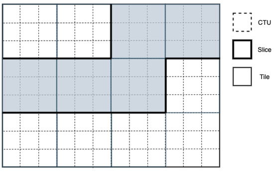
Figure 1.
Example of raster-scan slice partitioning (12 tiles, 3 raster-scan slices).
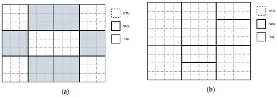
Figure 2.
Example of rectangular slice partitioning. (a) 12 tiles (4 columns, 3 rows) and 9 slices; (b) 6 tiles (3 columns, 3 rows) and 7 slices.
3.3. Subpictures in VVC
In VVC, a new frame partitioning tool, named subpictures, is introduced. A subpicture covers a rectangular frame sub-region consisting of one or more rectangular slices, as shown in Figure 3. Additionally, a subpicture can be specified as extractable—whereby no dependencies exist between current subpicture and subpictures within the same frame or subpictures in previous frames—or non-extractable. In both cases, whether in-loop filtering across each subpicture’s boundaries will be applied or not can be defined by the encoder.
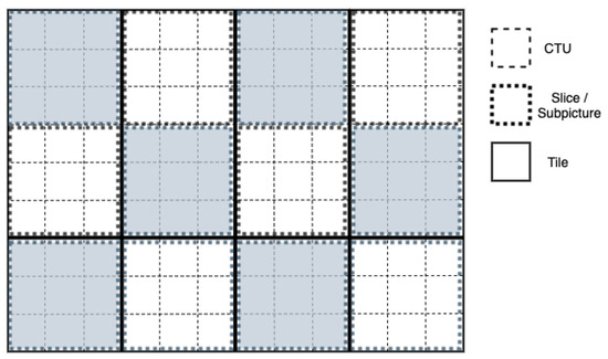
Figure 3.
Example of subpicture partitioning (4 × 2 tiles, 12 slices/subpictures).
As already mentioned, the basic structural unit of a subpicture is the rectangular slice, where a rectangular slice can either contain a number of tiles or a number of consecutive CTUs within a tile. In that sense, the combination of subpictures and tiles can be achieved through rectangular slices. Since within a tile, a number of rectangular slices can be defined, it is possible to have multiple subpictures within a tile, while the exact opposite is also possible, where a subpicture can contain a number of tiles that collectively form a rectangular slice. As can be seen in Figure 3, the boundaries of a subpicture do not always coincide with tile boundaries. While it is inevitable for some of the vertical subpicture boundaries to align with vertical tile boundaries, since a number of tile rows can form a rectangular slice, the top or bottom horizontal boundaries of subpictures may never coincide with horizontal tile boundaries.
Extractable subpictures are conceptually similar to MCTSs in HEVC. Like MCTSs, subpictures support independent encoding/decoding and extraction of a certain area within a frame, a useful functionality for applications such as viewport-dependent 360° video and region of interest (ROI). However, subpictures and MCTSs do not share the same design. An important difference between MCTSs and subpictures lies in the fact that motion vectors (MVs) in subpictures can point outside of subpicture boundaries, whether a subpicture is extractable or not, thereby favoring coding efficiency. In case of extractable subpictures, sample padding is applied to subpicture boundaries in the decoder. Additionally, the extraction of a number of subpictures does not require rewriting of the slice headers, as is the case with HEVC MCTSs. Since a frame can contain at least one slice which carries a significant amount of data, removing slice headers rewriting relieves the underlying burden in application systems.
4. Image Segmentation
Image segmentation is one of the most important techniques used to extract relevant information from an image, dividing the image into multiple segments representing the sub-areas or the objects of which an image consists [26]. In a sense, an image segmentation process is applied in order to simplify an image, so it is easier to evaluate or detect a region of interest (ROI). Most of the existing algorithms for image segmentation [27] are based on two fundamental properties of intensity, which are discontinuity and similarity [26]. As far as discontinuity is concerned, segmentation of an image is carried out based on abrupt changes in intensity. An example that falls into this category is edge detection. Regarding the second approach, based on similarity, an image is segmented into sub-areas that can be characterized as similar based on certain criteria. Methods that fall into this category are, for example, region split and merge, region growing as well as thresholding [28,29,30]. Thresholding is a simple, yet the most intuitive and effective, segmentation method used for partitioning an image into a foreground and a background. Gray levels regarding an object within an image are utterly different from gray levels. In this regard, thresholding utilizes those gray levels in order to categorize image pixels into two groups, distinguishing the foreground from the background [31,32]. Thresholding methods that have been proposed in the literature can be divided in two categories, namely global and local. Global thresholding techniques apply a single threshold to the entire image, while local techniques apply separate threshold values to different image areas [33]. A traditional global thresholding technique, yet the most successful, which is broadly used in applications such as pattern recognition, document binarization and computer vision, is the Otsu method [34].
4.1. Otsu Method
In the Otsu method, a threshold that maximizes the so-called between-class-variance metric is searched. The basic idea is to find a suitable threshold that divides the image pixels into two categories based on pixels’ intensity. Apart from its optimality, due to the method used for determining the threshold, Otsu is also characterized by its simplicity. The simplicity of this technique lies in the fact that it is entirely based on calculations carried out on the histogram of the image. In order to calculate the best threshold for an image that will segment the image into a foreground and a background, using the Otsu method, a color image is first converted into a grayscale image and then the histogram of the image is calculated. Now, assume that a threshold k is chosen, so that the image pixels are categorized into two classes, and [26]. In class , one finds the pixels with values in the range , while class is comprised of pixels with values in the range , where L denotes the distinct intensity values of that image. Using that threshold, the probability of a pixel belonging to the first class is
while the probability of a pixel belonging to the second class is
The mean values of pixel intensities regarding class and are
while the mean value of pixel intensities for the whole image is
Substituting with previous results, the above can also be expressed as [35]
and
Additionally, the variances of classes and are
while the total variance is
and the between class variance, which in the Otsu method is maximized, is expressed as
Class separability is also expressed as
For each k value , the aforementioned probabilities and mean values are calculated, while the value of is also determined for each value of k. The best threshold is then decided so that is maximized.
4.2. Region-Growing Method
Another simple, yet fast and effective image segmentation technique is region growing. In the region-growing method, a connected image region is extracted based on certain criteria, such as pixel intensity. The conventional approach of the region growing technique requires the manual selection of a set of initial seed points, which can be composed either of a single pixel or a group of connected pixels, and the extraction of neighboring pixels based on a similarity condition. Following this process, the method starts from an initial point and adds pixels to the selected region until the condition is no longer met. When the process of growing a certain region stops, another pixel that is not yet included in any other region is selected, and the process continues until all pixels are assigned to a region. The main advantage of this image segmentation technique is the formation of connected image regions. The basic algorithm of the region growing method based on 8-connectivity can be described as follows [26].
Let f(x, y) denote an input image, S(x, y) denote a seed array containing ones at the locations of seed points and zeroes elsewhere, and Q denote a predicate to be applied at each location (x, y). Arrays f and S are assumed to be of the same size.
- Find all connected components in S(x, y). Reduce each connected component to one pixel and mark these pixels as one. All other pixels in S will be marked as zero.
- Form an image where, at each point (x,y), if a certain condition is satisfied, Q, at those coordinates, and otherwise.
- Let g be the resulted image of appending each seed point in S all the points that have a value of one in and are 8-connected to that seed point.
- Assign each connected component in g to a different region by labeling them (e.g., integers or letters). This is the obtained segmented image after performing region growing.
Many variations of the conventional region-growing algorithm have been developed regarding both seed selection and homogeneity criteria. These variations include automatic seed selection and integration of Otsu thresholding.
5. Proposed Image Segmentation Methods
In the proposed content-aware subpicture segmentation methods, a frame of a video sequence is treated as a grayscale image, and segmentation techniques inspired by image segmentation are utilized in order to partition a frame into a number of spatially uniform areas that represent the desired number of subpictures. More precisely, in the first step of each of the proposed segmentation algorithms, Otsu thresholding is applied in order to separate the image into foreground and background areas, resulting in a binary image where 0 values represent pixels belonging in the background, while values of 255 represent pixels belonging in the foreground. In the next step, region growing is utilized to define the desired number of subpictures. However, since the conventional region-growing method operates on a pixel level, proposed region-growing methods are appropriately modified in order to operate on a CTU-level and be rendered compatible with the VVC video coding standard. In that sense, a CTU map is created, where for each CTU, the mean value of the resulted Otsu thresholding pixel values is calculated, normalized (in the range between zero and one) and used as input to the two proposed region growing methods, namely Serial Region Growing and Concurrent Region Growing.
5.1. Serial Region Growing
In the first method, presented in Algorithm 1, the target number of foreground and background areas are initialized and region growing with automatic seed selection is subsequently performed, starting with defining the foreground areas. In the first step, the most homogeneous CTU in the foreground is searched, serving as the initial seed point, and during Region Growing, homogeneous sub-picture areas are grouped together, where each initial seed area grows in the upper, lower, left or right direction. In order to grow a region in a direction, the value of each CTU from the aforementioned CTU map that will be added to the current area must be larger than a threshold. Note that this threshold is tunable. As fine frame partitioning leads to a disproportionate decrease in video compression efficiency, a restriction is posed by the algorithm concerning the minimum size of a region. Therefore, only areas that are larger than or equal to a predefined size are kept, while smaller areas are discarded. It is important to mention that an area grows until the threshold criterion is no longer met in any direction before proceeding to the next area. After defining the target foreground areas, the above-mentioned process is repeated for background areas, where the most homogeneous CTUs in the background are utilized as seed points for region growth. During the next stage of the algorithm, the defined foreground and background areas are expanded in order to cover the whole frame area. It is possible that fewer than the target areas are detected. In the final stage of the algorithm, splitting of the largest areas of the frame takes place at the point where the difference of average CTU map values is maximized until the desired number of subpictures is reached.
| Algorithm 1 Serial Region Growing |
|
5.2. Concurrent Region Growing
In the second method, presented in Algorithm 2, the CTU map values are sorted in descending order, from the most homogeneous CTUs to the foreground to the most homogeneous in the background, and a number of initial seed points equal to the number of target number of subpictures, are automatically determined based on the descending order. A restriction concerning the minimum distance between the selected seed points is considered in order to avoid the formation of very small regions as justified in Section 5.1. In that sense, whenever a seed candidate is selected, the minimum distance restriction must be met. If not, the algorithm proceeds with the next CTU seed candidate. After defining the seed points, region growing is applied to each of the defined areas, where rectangular regions are expanded either in the top, bottom, left or right direction. One step of region growing is performed for each area in each iteration, meaning that an area does not need to be fully expanded before proceeding to the next. The criterion by which a rectangular area is expanded, as well as in which direction it will be expanded, is variance. For all available choices, the variance of each new rectangular area is calculated and the direction that yields the minimum variance is chosen. The algorithm terminates when no more expansion options are to be considered, meaning that either frame borders are reached, or the current area collides with another rectangular area.
After the sub-picture areas have been defined, since subpictures’ boundaries need to comply with slice boundaries and slices are defined either as a subset of a tile or a collection of tiles, tiles and slices need to be appropriately determined. An additional restriction posed by the VVC standard is that all CTUs of a subpicture must belong to the same tile and all CTUs in a tile must belong to the same subpicture. In this regard, tile/slice partitioning methods are introduced and more specifically, a straightforward method is proposed, along with two cost effective partitioning methods for avoiding over-partitioning of a frame, namely Tile-oriented petitioning, Slice-oriented partitioning and Adjusted Slice-oriented partitioning, respectively.
| Algorithm 2 Concurrent Region Growing |
|
5.3. Tile-Oriented Partitioning
The most straightforward approach is to define tile lines based on the subpicture borders. However, this would create unnecessary partitions, leading to both loss of quality and bitrate increase. As such, adaptive ways of frame partitioning need be developed.
5.4. Slice-Oriented Partitioning
The first adaptation to the straightforward tile partitioning takes advantage of the fact that many rectangular slices can exist in a tile, allowing for the employment of more robust and efficient tile partitioning where fewer tiles are defined. Taking this fact into consideration, the following is proposed concerning the tile grid. For each subpicture, vertical border lines serve as vertical borders for tiles. Regarding the horizontal borders of tiles, only horizontal borders of subpictures that cut vertical borders of tiles are considered. In all other cases, the horizontal borders of subpictures serve as borders of slices within a tile. An example of this method is provided in Figure 4, where a frame is divided into four subpictures, where different colors represent different subpicture areas and solid lines represent the subpicture borders. According to the proposed slice-oriented partitioning method, each horizontal subpicture border serves as a slice border, instead of a horizontal tile border (indicated by the dashed lines) that would be the outcome of the straightforward tile partitioning.
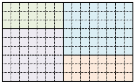
Figure 4.
Example of proposed Slice-oriented partitioning (4 subpictures, 2 tiles, 6 slices).
5.5. Adjusted Slice-Oriented Partitioning
This tile partitioning method, which is an adaption of the previous method, focuses on reducing the number of vertical lines drawn. This can be achieved by adjusting the boundaries of the subpicture areas that have close vertical boundaries by employing a threshold, T. If the CTU distance between two vertical boundaries is lower than or equal to the threshold T, the boundaries are adjusted to be the same. Since this step serves as a final fine-tuning stage, the initial subpictures generated by the Serial and Concurrent Region Growing algorithms need to be kept almost intact. For this reason, in experiments, threshold T is set to one. As shown in Figure 5, since the boundaries of the gray and the blue subpictures have a distance of one, both the right and the left vertical borders of the orange and the blue subpictures, respectively, are moved to the right by one CTU column, reducing the number of vertical tile lines needed to define the subpicture areas.
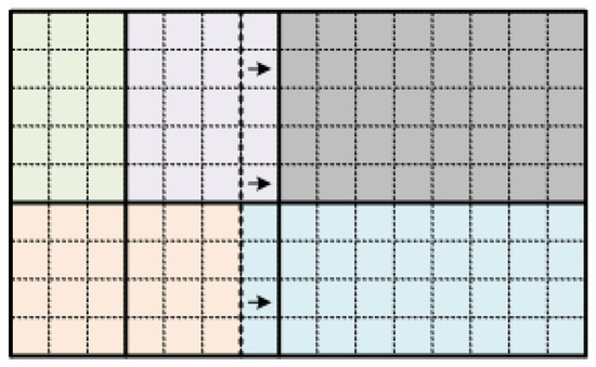
Figure 5.
Example of proposed Adjusted Slice-oriented partitioning (5 subpictures, 6 tiles, 6 slices).
5.6. Visual Examples of Proposed Segmentation Methods
In Figure 6, Figure 7, Figure 8, Figure 9 and Figure 10, visual examples for the proposed image segmentation methods are provided. Since the proposed algorithms differ in terms of initial seed point selection and region growing methodology, different results are produced depending on the image complexity and target number of subpictures.
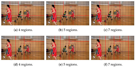
Figure 6.
BasketballDrive video sequence: (a–c) Serial Region Growing, (d–f) Concurrent Region Growing.
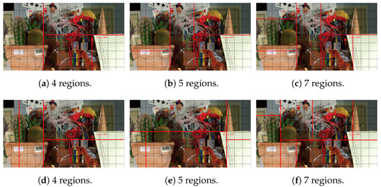
Figure 7.
Cactus video sequence: (a–c) Serial Region Growing, (d–f) Concurrent Region Growing.
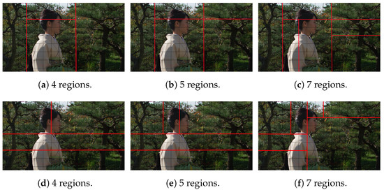
Figure 8.
Kimono video sequence: (a–c) Serial Region Growing, (d–f) Concurrent Region Growing.
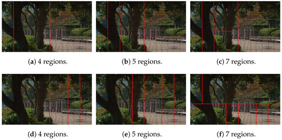
Figure 9.
Parkscene video sequence: (a–c) Serial Region Growing, (d–f) Concurrent Region Growing.
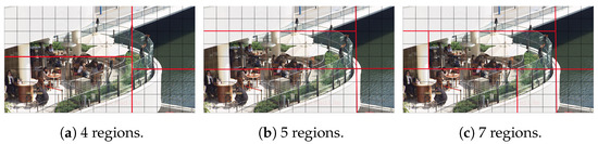
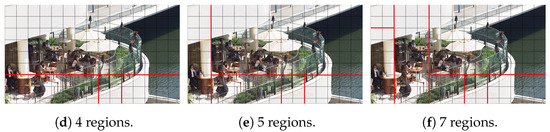
Figure 10.
BQTerrace video sequence: (a–c) Serial Region Growing, (d–f) Concurrent Region Growing.
In Figure 6 one may see the impact of the two proposed subpicture partitioning algorithms for the test sequence BasketballDrive. As can be seen, this is an example with a big proportion of the frame in the background. The background can be divided to two distinct, rather homogeneous areas. In this case, the first proposed algorithm (Figure 6a–c), which in general seems to favor homogeneous areas, detects these two (background) areas as two subpictures. The rest of the subpictures are formed by splitting these subpictures in a way that the new subpictures created includes areas with the highest possible homogeneity. On the other hand, the second algorithm (Figure 6d–f), which starts by growing all areas concurrently, has to split the frame into a specific number of subpictures from the beginning. As a result, it can detect areas with players more efficiently.
Concerning the Cactus video sequence, Figure 7, as can be observed, object areas are homogeneous, while the background is more complex. Concerning the first method, (Figure 7a–c), since the separation between objects is clearer, the algorithm is able to better detect objects of interest, cactus and paper, while in the second method, (Figure 7d–f), since homogeneous CTUs are detected within objects and the region growing of each area happens concurrently, the object separation performance falls behind compared to the first method.
In Figure 8, the image segmentation results for Kimono are depicted. This video sequence is characterized by a large homogeneous background area, the trees behind the geisha. Again, the first algorithm (Figure 8a–c), (in case of four subpictures) detects and separates the background on the right and left side of the geisha, as well as the top of her head, into different subpictures, while her face and body is assigned to a different subpicture. However the second method (Figure 8d–f) fails to detect the object of interest, and instead tries to cover the background areas.
In Figure 9, visual examples are provided for ParkScene video sequence. As can be observed, the ParkScene video sequence is also characterized by a complex background. Again, the first method (Figure 9a–c), is able to detect and separate the homogeneous areas, the floor and the trees, while in the second method, (Figure 9d–f), since the most homogeneous CTUs fall into those regions, the most homogeneous areas tend to be over-separated.
Lastly, in the BQTerrace video sequence, Figure 10, more sharp contrasts exist; there are white and dark areas within the frame. Concerning, the first method, (Figure 10a–c), a good partitioning is achieved by grouping together homogeneous areas, while in the second method, (Figure 10d–f), the most homogeneous CTUs that serve as seed points are very close, resulting in over-partitioning of homogeneous areas.
6. Evaluation Metrics
In order to evaluate the proposed segmentation methods, we used an unsupervised objective evaluation method. Unsupervised evaluation methods offer the potential to evaluate segmentation algorithms in the absence of ground truth concerning the segmented images, while also enabling the objective comparison of different segmentation algorithms [36]. Additionally, unsupervised evaluation is critical in real-time segmentation, while supporting also adaptive segmentation schemes where the algorithm parameters are self-adjusted according to evaluation results. Concerning unsupervised evaluation, the criteria that need to be met [37] are:
- i
- The regions must be uniform and homogeneous with respect to some characteristic(s).
- ii
- Adjacent regions must have significant differences with respect to the characteristic(s) on which they are uniform.
- iii
- Region interiors should be simple and without holes.
- iv
- Boundaries should be simple, not ragged, and be spatially accurate.
With respect to the first criterion, the unsupervised method used for evaluation in this paper, namely Zeboudj’s contrast [38], utilizes the internal contrast , Equation (13), to measure the degree to which a region is uniform. The internal contrast is defined as the average max contrast in a specific region, noted as , where max contrast is defined as the largest luminance difference between a pixel, s, and its neighboring pixels, noted as W(s) in the same region. In Equation (13), denotes the surface of a region .
Concerning the second criterion, Zeboudj’s contrast evaluation method uses the external contrast (14), to measure the inter-region disparity, where is defined as the average max contrast for all border pixels in that region, where max contrast is the largest difference in luminance between a pixel and its neighboring pixels in separate regions. In (14), denotes the border (of length ) of a region .
To evaluate the whole image, the intra-region as well as the inter-region metrics must be combined for each individual region. The contrast of a region (15) is:
In the next step, the global contrast (16) of the whole image is calculated.
Since the proposed algorithms are CTU based, the following assumptions were made, regarding Equations (13) and (14):
- : Region of CTUs
- : CTUs
- : The set of CTUs neighboring to s
- Luminance: The average luminance of all pixels within a CTU.
Concerning criteria (iii) and (iv), they are satisfied, since the definition of subpictures involves continuous regions, while their boundaries are inherently simple, not ragged and spatially accurate. Finally, in the experiments, the outcome of the proposed algorithms is evaluated in terms of PSNR and bitrate. Concerning measurement of PSNR, Mean Square Error (MSE) between the pixels of the coded picture and the original uncompressed one is calculated. The PSNR of the whole video is then calculated by averaging over PSNRs of frames. It should be noted that PSNR calculation is embedded in Reference Software used and no changes were made by authors in this field.
7. Experiments
Setup
In order to evaluate the proposed subpicture assignment schemes, we used the VVC Test Model (VTM) 11.2 reference software [39] and the Common test conditions [40] for the Low Delay P configuration with QP = 32. Experiments were conducted on a Linux Server with 2 10-core Intel(R) Xeon(R) Silver 4210 CPUs running at 2.20 GHz.
The first set of experiments aimed to show the impact of each parameter of the proposed algorithms. For this set of experiments, we encoded the first 100 frames of the class B common test sequences [41] listed in Table 1. Concerning Serial Region Growing, the algorithm used two tunable thresholds, one regarding background/foreground, and the other, the minimum area a subpicture may occupy. After the first step of the Serial Growing algorithm, each CTU is assigned a value ranging from 0 to 1. Values close to zero are thought to be background values, while values close to one are considered foreground values. The first threshold T is used to determine the closeness of these values to the limit for each case. In Table 2, we summarize the experimental results for different values of T, 5 subpictures, and minimum area . In order to determine the impact of the threshold regarding the size of the minimum area in Serial Region Growing, experiments were also conducted for different values of the minimum area threshold, ranging from to for 5 subpictures and threshold T set to 0.5. Their results are presented in Table 3. Finally, concerning the minimum distance parameter in Concurrent Region Growing, experimental results are shown in Table 4 for different values of the minimum distance parameter, ranging from 1 to 5.

Table 1.
CTS video sequences.
Table 2.
PSNR (dB) and bitrate (bps) for different values of T.
Table 3.
PSNR (dB) and bitrate (bps) for different values of minimum area.
Table 4.
PSNR (dB) and Bitrate (bps) for different values of minimum distance.
With the next set of experiments we studied the comparative impact of the two proposed algorithms regarding video coding performance. For these experiments, the thresholds of each proposed algorithm were set as follows. For the Serial Region Growing Algorithm, threshold which is the mid allowable value, as T varies from 0 to 1 and minimum area size was set to CTUs, while for the Concurrent Region Growing, the minimum distance between successive seed points was set to 3 CTUs. The values for both minimum size area and minimum distance were chosen so as to lead to minimum areas that are usually met in frame partitioning algorithms in video coding (i.e., nearly no smaller than 10% of the total frame area).
Figure 11, Figure 12 and Figure 13 plot the average bitrate performance, while Figure 14, Figure 15 and Figure 16 plot the average YUV-PSNR performance for all the video sequences presented in Table 1 for 4, 5 and 7 regions, respectively.
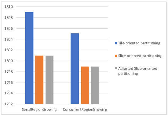
Figure 11.
Average bitrate performance for 4 regions.
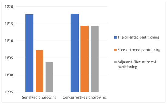
Figure 12.
Average bitrate performance for 5 regions.
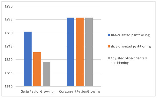
Figure 13.
Average bitrate performance for 7 regions.
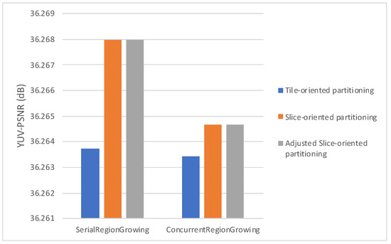
Figure 14.
Average YUV-PSNR performance 4 regions.
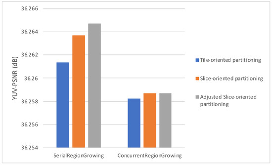
Figure 15.
Average YUV-PSNR performance 5 regions.
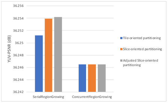
Figure 16.
Average YUV-PSNR performance for 7 regions.
Experimental results show, as indicated in Figure 11, Figure 12, Figure 13, Figure 14, Figure 15 and Figure 16, Serial Region Growing achieves slightly better compression efficiency. This result is in complete agreement with the visual results presented in Section 5. As the Serial Region Growing Subpicture Partitioning method manages to detect better objects in the foreground and has a more precise partitioning regarding foreground and background, subpictures produced contain content that can be compressed more efficiently. At the same time, the cost from the breaking of dependencies among subpictures is smaller compared to that of having subpictures that share similar content.
To further study the effects of the proposed segmentation algorithms, we have also conducted experiments for the sequences of the Ultra Video Group (UVG) dataset [42] presented in Table 5, using the same parameter configuration as above. As results indicate in Figure 17 and Figure 18, the same trend can be observed, where the Serial Region Growing algorithm exhibits a relatively superior compression performance compared to the Concurrent Region Growing algorithm.
Table 5.
UVG video sequences.
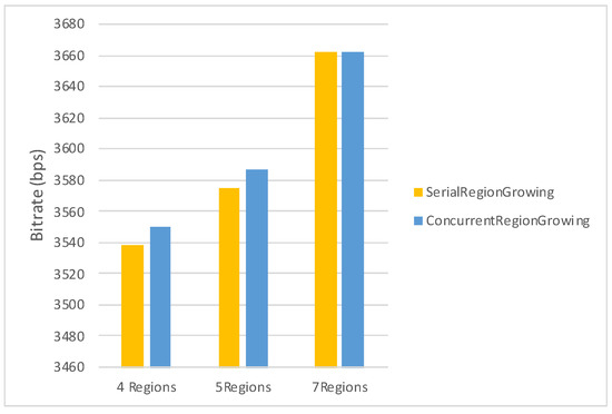
Figure 17.
Average bitrate performance for 4, 5 and 7 regions (UVG dataset).
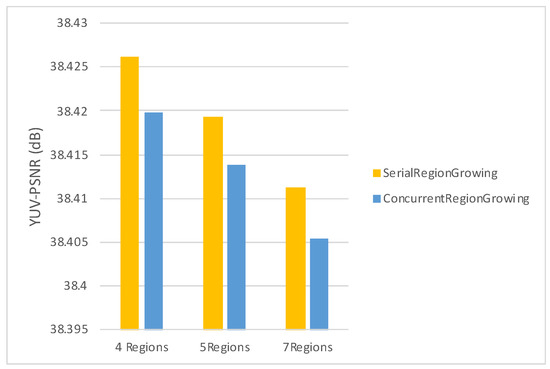
Figure 18.
Average YUV-PSNR performance for 4, 5 and 7 regions (UVG dataset).
In order to verify the stability of the proposed algorithms, experiments with an extreme number of areas were conducted. It should be noted that the case of 135 areas means that each area contains only one CTU. The results presented in Table 6 indicate that the presented algorithms are robust regarding their segmentation ability, as they manage to create an unrealistic number of partitions without collapsing. It can also be noticed that for a large number of areas, compression efficiency is better for the Concurrent Region Growing algorithm. This is due to the fact that in order to achieve a segmentation with large number of areas, the thresholds concerning minimum area for the Serial Region Growing algorithm and minimum distance for the Concurrent Region Growing algorithm had to be minimized. Therefore neighboring CTUs could be selected as seeds which could lead to very small areas. As the Serial Region Growing algorithm begins with one seed, grows the area and then proceeds to the seed of the next area, it tends to form big areas in the beginning and very small areas (even areas with just one CTU) as the algorithm progresses. On the other hand, for the Concurrent Region Growing algorithm, the probability of forming extremely small areas tends to be smaller, since all seed points are selected simultaneously, and the areas are expanded concurrently.
Table 6.
PSNR (dB) and Bitrate (bps) for extreme number of areas.
Moreover, concerning the slice/tile partitioning schemes, Figure 11, Figure 12, Figure 13, Figure 14, Figure 15 and Figure 16, which refer to the first set of experiments, indicate that the proposed methods lead to bitrate savings, with Slice-oriented Partitioning and Adjusted Slice-oriented Partitioning producing fairly similar results. This can be explained by the fact that both tile/slice partitioning methods aim to reduce bitrate. Slice-oriented Partitioning achieves that by avoiding drawing redundant lines, while Adjusted Slice-oriented Partitioning adjusts the subpicture borders so that a more cost effective, in terms of coding efficiency, slice/tile partitioning can be adopted. Adjusted Slice-oriented Partitioning further increases the compression rate compared to Slice-oriented Partitioning, with a minor loss in terms of PSNR. It should be noted that the initial subpicture partitioning may be such that all or some of the aforementioned schemes lead to the same slice/tile grid. This is the case met in the second set of experiments; therefore, in Figure 17 and Figure 18 results are presented only for the region growing algorithms, as all partitioning schemes exhibited the same performance.
Furthermore, Table 7 and Table 8 summarize the difference between the proposed segmentation and partitioning algorithms for 4, 5 and 7 regions on the one side and the VVC encoder without any partitioning scheme (i.e., subpictures, tiles, slices) as baseline on the other. As it can be seen, proposed methods have minor impact on video quality and compression efficiency, with PSNR degradation ranging from 0.006 to 0.028 dB and Bitrate increment from 2% to 5%, respectively.
Table 7.
PSNR (dB) difference between proposed algorithm and baseline VVC encoder.
Table 8.
Bitrate difference between proposed algorithm and baseline VVC encoder.
One issue we have come across is that there is no ground truth for the standard test sequences that the experiments are run on. Another issue to tackle is that the algorithms operate on video data, and as such, they are CTU based and not pixel based, unlike standard image segmentation algorithms. For the aforementioned reasons, unsupervised evaluation methods are used, and more particularly, the Zebdouj’s contrast metric is utilized in order to evaluate the performance of the introduced segmentation algorithms. The advantage of unsupervised methods is that the presence of a ground truth is not needed. Lastly, as both Region Growing proposed algorithms operate on 15 × 9 map where each point represents a CTU, and as such operates on a CTU level and not on a pixel level, we chose to calculate Zeboudj’s contrast contrast on image where each point represents a CTU’s average luma value instead of on the default image.
In Table 9 and Table 10, the Zebdouj’s global contrast is presented for 4, 5 and 7 regions for the CTS and UVG video datasets, respectively. As can easily be inferred by Equation (13) a higher Zeboudj’s contrast value amounts to a better segmentation. Experimental results for both video datasets indicate that the proposed Serial Region Growing Subpicture Partitioning algorithm yields a better performance. The general indication for the suitability of Serial Region Growing as a partitioning algorithm, derived by Zeboudj’s contrast metric, is correlated with the visual data for the segmentations shown in Figure 6, Figure 7, Figure 8, Figure 9 and Figure 10, where Serial Region Growing achieves segmentation that seems to be better adapted to the image’s contents. Finally, it should be noted that both proposed algorithms have a negligible impact on encoding time, as their execution time is in the order of milliseconds, when one frame’s encoding time in the baseline VVC encoder is in the order of tens of seconds.
Table 9.
Zeboudj’s contrast for 4, 5, 7 regions (Serial Region Growing, Concurrent Region Growing), CTS video sequences.
Table 10.
Zeboudj’s contrast for 4, 5, 7 regions (Serial Region Growing, Concurrent Region Growing), UVG video sequences.
8. Conclusions
In this paper, we proposed two image segmentation algorithms, Serial and Concurrent Region Growing, suitable for video data in order to provide subpictures with independent contents during video encoding. To the best of our knowledge, this is the first time that image segmentation techniques have been used for content-aware subpicture partitioning in VVC video encoding. Additionally, tile/slice partitioning adjustments were developed with the aim of reducing the bitrate by foregoing definition of redundant slice and tiles. The algorithms were then evaluated with Zebdouj’s contrast. Further evaluation of the algorithms, as well as the tile/slice partitioning schemes, took place in terms of bitrate and psnr. Overall, Serial Region Growing was shown to be the most suitable algorithm for the most common cases, both in terms of segmentation accuracy and video coding efficiency. However, in extreme cases, where a large number of subpictures is desired, Concurrent Region Growing produces better results in terms of compression efficiency and video quality. Last but not least, the tile/slice partitioning adjustments helped to alleviate some of the bitrate increase introduced by employing subpicture partitioning during the encoding scheme.
Author Contributions
Conceptualization, N.P.; methodology, N.P., P.B. and M.K.; software, P.B.; validation, N.P. and P.B.; writing—original draft preparation, N.P., P.B. and M.K.; writing—review and editing, N.P. and M.K.; supervision, M.K. All authors have read and agreed to the published version of the manuscript.
Funding
This research received no external funding.
Conflicts of Interest
The authors declare no conflict of interest.
References
- Bross, B.; Chen, J.; Ohm, J.R.; Sullivan, G.J.; Wang, Y.K. Developments in international video coding standardization after AVC, with an overview of Versatile Video Coding (VVC). Proc. IEEE 2021, 109, 1463–1493. [Google Scholar] [CrossRef]
- Wang, Y.K.; Skupin, R.; Hannuksela, M.M.; Deshpande, S.; Drugeon, V.; Sjöberg, R.; Choi, B.; Seregin, V.; Sanchez, Y.; Boyce, J.M.; et al. The High-Level Syntax of the Versatile Video Coding (VVC) Standard. IEEE Trans. Circuits Syst. Video Technol. 2021, 31, 3779–3800. [Google Scholar] [CrossRef]
- Sidaty, N.; Hamidouche, W.; Déforges, O.; Philippe, P.; Fournier, J. Compression performance of the versatile video coding: HD and UHD visual quality monitoring. In Proceedings of the 2019 Picture Coding Symposium (PCS), Ningbo, China, 12–15 November 2019; pp. 1–5. [Google Scholar]
- Sullivan, G.J.; Ohm, J.; Han, W.; Wiegand, T. Overview of the High Efficiency Video Coding (HEVC) Standard. IEEE Trans. Circuits Syst. Video Technol. 2012, 22, 1649–1668. [Google Scholar] [CrossRef]
- Chen, J.; Ye, Y.; Kim, S. Algorithm description for Versatile Video Coding and Test Model 10 (VTM 10). In Proceedings of the JVET Meeting, no. JVET-S2002. ITU-T and ISO/IEC, Teleconference, Online, 22 June–1 July 2020. [Google Scholar]
- Skupin, R.; Sanchez, Y.; Sühring, K.; Schierl, T.; Ryu, E.; Son, J. Temporal mcts coding constraints implementation. In Proceedings of the 120th MPEG Meeting of ISO/IEC JTC1/SC29/WG11, MPEG, Macao, China, 23–27 October 2017; Volume 120, p. m41626. [Google Scholar]
- Otsu, N. A threshold selection method from gray-level histograms. IEEE Trans. Syst. Man Cybern. 1979, 9, 62–66. [Google Scholar] [CrossRef]
- Adams, R.; Bischof, L. Seeded Region Growing. IEEE Trans. Pattern Anal. Mach. Intell. 1994, 16, 641–647. [Google Scholar] [CrossRef]
- Jianzhuang, L.; Wenqing, L.; Yupeng, T. Automatic thresholding of gray-level pictures using two-dimension Otsu method. In Proceedings of the 1991 International Conference on Circuits and Systems, Shenzhen, China, 16–17 June 1991; pp. 325–327. [Google Scholar]
- WU, Y.q.; Zhe, P.; WU, W.Y. Image thresholding based on two-dimensional histogram oblique segmentation and its fast recurring algorithm. J. Commun. 2008, 29, 77. [Google Scholar]
- Huang, M.; Yu, W.; Zhu, D. An improved image segmentation algorithm based on the Otsu method. In Proceedings of the 2012 13th ACIS International Conference on Software Engineering, Artificial Intelligence, Networking and Parallel/Distributed Computing, Kyoto, Japan, 8–10 August 2012; pp. 135–139. [Google Scholar]
- Jun, Z.; Jinglu, H. Image segmentation based on 2D Otsu method with histogram analysis. In Proceedings of the 2008 International Conference on Computer Science and Software Engineering (CSSE), Wuhan, China, 12–14 December 2008; Volume 6, pp. 105–108. [Google Scholar] [CrossRef]
- Xiao, L.; Ouyang, H.; Fan, C. An improved Otsu method for threshold segmentation based on set mapping and trapezoid region intercept histogram. Optik 2019, 196, 163106. [Google Scholar] [CrossRef]
- Sha, C.; Hou, J.; Cui, H. A robust 2D Otsu’s thresholding method in image segmentation. J. Vis. Commun. Image Represent. 2016, 41, 339–351. [Google Scholar] [CrossRef]
- Chen, Q.; Zhao, L.; Lu, J.; Kuang, G.; Wang, N.; Jiang, Y. Modified two-dimensional Otsu image segmentation algorithm and fast realisation. IET Image Process. 2012, 6, 426–433. [Google Scholar] [CrossRef]
- Tremeau, A.; Borel, N. A region growing and merging algorithm to color segmentation. Pattern Recognit. 1997, 30, 1191–1203. [Google Scholar] [CrossRef]
- Shih, F.Y.; Cheng, S. Automatic seeded region growing for color image segmentation. Image Vis. Comput. 2005, 23, 877–886. [Google Scholar] [CrossRef]
- Fan, J.; Yau, D.K.; Elmagarmid, A.K.; Aref, W.G. Automatic image segmentation by integrating color-edge extraction and seeded region growing. IEEE Trans. Image Process. 2001, 10, 1454–1466. [Google Scholar] [CrossRef] [PubMed]
- Hojjatoleslami, S.A.; Kittler, J. Region growing: A new approach. IEEE Trans. Image Process. 1998, 7, 1079–1084. [Google Scholar] [CrossRef] [PubMed]
- Wang, X.; Xue, Y. Fast HEVC intra coding algorithm based on Otsu’s method and gradient. In Proceedings of the 2016 IEEE International Symposium on Broadband Multimedia Systems and Broadcasting (BMSB), Nara, Japan, 1–3 June 2016; pp. 1–5. [Google Scholar]
- Gharghory, S.M. Optimal Global Threshold based on Two Dimension Otsu for Block Size Decision in Intra Prediction of H. 264/AVC Coding. Int. J. Adv. Comput. Sci. Appl. 2019, 10, 177–185. [Google Scholar] [CrossRef]
- Wang, W.; Duan, L.; Wang, Y. Fast image segmentation using two-dimensional Otsu based on estimation of distribution algorithm. J. Electr. Comput. Eng. 2017, 2017, 1735176. [Google Scholar] [CrossRef]
- Nie, F.; Wang, Y.; Pan, M.; Peng, G.; Zhang, P. Two-dimensional extension of variance-based thresholding for image segmentation. Multidimens. Syst. Signal Process. 2013, 24, 485–501. [Google Scholar] [CrossRef]
- Liao, Y.W.; Lin, J.R.; Chen, M.J.; Chen, J.W. Fast depth coding based on depth map segmentation for 3D video coding. In Proceedings of the 2017 IEEE International Conference on Consumer Electronics-Taiwan (ICCE-TW), Taipei, Taiwan, 12–14 June 2017; pp. 135–136. [Google Scholar]
- Wiegand, T.; Sullivan, G.J.; Bjontegaard, G.; Luthra, A. Overview of the H. 264/AVC video coding standard. IEEE Trans. Circuits Syst. Video Technol. 2003, 13, 560–576. [Google Scholar] [CrossRef]
- Gonzalez, R.C.; Woods, R.E. Digital Image Processing; Publishing House of Electronics Industry: Beijing, China, 2002. [Google Scholar]
- Lin, P.D.J. Survey on the Image Segmentation Algorithms. In Proceedings of the International Field Exploration and Development Conference, Qingdao, China, 16–18 September 2021. [Google Scholar]
- Pham, D.L.; Xu, C.; Prince, J.L. Current methods in medical image segmentation. Annu. Rev. Biomed. Eng. 2000, 2, 315–337. [Google Scholar] [CrossRef]
- Sharma, N.; Mishra, M.; Shrivastava, M. Colour Image Segmentation Techniques and Issues: An Approach. Int. J. Sci. Technol. Res. 2012, 1, 9–12. [Google Scholar]
- Khan, W. Image Segmentation Techniques: A Survey. J. Image Graph. 2014, 1, 166–170. [Google Scholar] [CrossRef]
- Milstein, N. Image segmentation by adaptive thresholding. Tech. Isr. Inst. Technol. Fac. Comput. Sci. 1998, 15, 2014. [Google Scholar]
- Bhargavi, K.; Jyothi, S. A Survey on Threshold Based Segmentation Technique in Image Processing. Int. J. Innov. Res. Dev. 2014, 3, 234–239. [Google Scholar]
- Leedham, G.; Chen, Y.; Takru, K.; Tan, J.H.N.; Mian, L. Comparison of Some Thresholding Algorithms for Text/Background Segmentation in Difficult Document Images. In Proceedings of the Seventh International Conference on Document Analysis and Recognition (ICDAR 2003), Edinburgh, UK, 6 August 2003; p. 859. [Google Scholar]
- Chaki, N.; Shaikh, S.H.; Saeed, K. A comprehensive survey on image binarization techniques. Explor. Image Bin. Tech. 2014, 560, 5–15. [Google Scholar]
- Senthilkumaran, N.; Vaithegi, S. Image segmentation by using thresholding techniques for medical images. Comput. Sci. Eng. Int. J. 2016, 6, 1–13. [Google Scholar]
- Zhang, H.; Fritts, J.E.; Goldman, S.A. Image segmentation evaluation: A survey of unsupervised methods. Comput. Vis. Image Underst. 2008, 110, 260–280. [Google Scholar] [CrossRef]
- Haralick, R.M.; Shapiro, L.G. Image segmentation techniques. Comput. Vision, Graph. Image Process. 1985, 29, 100–132. [Google Scholar] [CrossRef]
- Chabrier, S.; Emile, B.; Laurent, H.; Rosenberger, C.; Marché, P. Unsupervised evaluation of image segmentation application to multi-spectral images. In Proceedings of the 17th International Conference on Pattern Recognition, Cambridge, UK, 26 August 2004; Volume 1, pp. 576–579. [Google Scholar] [CrossRef]
- VTM VVC Reference Software. Available online: https://vcgit.hhi.fraunhofer.de/jvet/VVCSoftware_VT (accessed on 27 June 2022).
- Boyce, J.; Suehring, K.; Li, X.; Seregin, V. JVET-J1010: JVET Common Test Conditions and Software Reference Configurations; Technical Report JVET-J1010; JVET: San Diego, CA, USA, 2018. [Google Scholar]
- Bossen, F. Common test conditions and software reference configurations. In Proceedings of the Joint Collaborative Team on Video Coding (JCT-VC) of ITU-T SG16 WP3 and ISO/IEC JTC1/SC29/WG11 (JCTVC-L1100), Geneva, CH, USA, 21–28 July 2010. [Google Scholar]
- Mercat, A.; Viitanen, M.; Vanne, J. UVG dataset: 50/120fps 4K sequences for video codec analysis and development. In Proceedings of the 11th ACM Multimedia Systems Conference, Istanbul, Turkey, 8–11 June 2020; pp. 297–302. [Google Scholar]


Publisher’s Note: MDPI stays neutral with regard to jurisdictional claims in published maps and institutional affiliations. |
© 2022 by the authors. Licensee MDPI, Basel, Switzerland. This article is an open access article distributed under the terms and conditions of the Creative Commons Attribution (CC BY) license (https://creativecommons.org/licenses/by/4.0/).