Abstract
In an industrial mass production pattern, quality prediction is one of the important processes when guarding quality. The products are extracted periodically or quantitatively for inspection in order to observe the relationship between process variation and engineering specification. When these irregularities are not instantly detected by lot sampling inspection, lot defectives are produced, and the defective cost increases. Failure to identify defects during sampling inspection leads to product returns or harm to business reputation. Press casting is a common mass production method in the metal industry. After the metal is molten at a high temperature, high pressure is injected into the mold, and then it is solidified and formed in the mold. Thus, pressure stability inside the mold is one of the key factors that influences quality. The melting point of aluminum alloy is normally around 650 °C, but there was no sensor that could withstand this high temperature. To combat this, we developed a high temperature resistant sensor and installed it into pressure casting mold grounded on the principles of fluid mechanics and experts’ suggestions in order to realize the impact of pressure change on the mold. To our limited knowledge, it was a seminal study on predicting mold’s casting quality via in-mold pressure data. We propose a press casting quality prediction method based on machine learning. By collecting the in-mold pressure data in real time. Savitzky-Golay Filter is used for data smoothing, and first-order difference is taken to extract the time interval of an actual injection of molten metal in-to the mold. We extract the key data that influence the quality and employ XGBoost to establish a classifier. In the experiment we prove that the method achieves good accuracy of quality prediction and recall of defectives for in-mold pressure. Via this model, we not only can save large amount of time and costs, but also can carry out maintenance warnings in advance, notify professionals to stop produce defective products, reduce the shipping risk and maintain reputation so as to strengthen its competitive edge.
1. Introduction
Press casting is a common metalworking method, and its characteristic is that the metal is molten at a high temperature and injected into the mold under high pressure, so that it is solidified and formed in a mold. As the mold is filled very fast due to high pressure injection and the mold can be fully filled with molten metal, there is air retained inside the mold, forming gas holes. When the compression casting product yield is too low, posterior visual inspection is required, which fails in real-time monitoring and leads to a lot of rejections.
With the advancement of science and technology and the rise of artificial intelligence (AI) and machine learning in recent years, Yarlagadda and Chiang [1] used neural network to predict the press casting parameter setting in 1999. Anijdan [2] then employed a genetic algorithm and neural network to analyze how to design Al-Si cast alloy with minimum porosity in 2006, hoping to reduce the influence of porosity on the quality of cast products as much as possible.
Ageyeva and Horváth et al. (2019) indicated that the first key to Industry 4.0 is data, and in the production patterns generated by mold, the data most related to process control are from the inside of mold [3]. Farahani and Brown (2019) suggested that due to the rise of techniques correlated with Industry 4.0, manufacturers could combine the mass data derived from the production process with the data sourced from eight in-mold signals and four machine signals. Combining production knowledge and training models, the correlation between data and quality can be found to improve product quality and yield [4].
In terms of cast products, porosity is always one of the important parameters that influence the quality. Cao et al. (2017) studied the influence of different vacuum degrees on the porosity and mechanical properties of Al die castings [5]. Apparao et al. (2017) also proposed using the Taguchi method to optimize the press casting technique in [6]. In 2020, Aksoy used an AI method to evaluate the heat transfer coefficient of casting mold interface in the press casting process [7]. The above academic studies showed how to reduce the influence of porosity on the quality of cast products.
A technical report from Kistler Company showed that the internal pressure of noncrystalline plastic cavity drops fast in the holding stage, whereas the internal pressure of partial crystalline plastic cavities drops smoothly in the holding stage, and the internal pressure drops greatly until the gate is solidified. As the mold temperature has not yet reached stable equilibrium at the initial stage of injection, and plastic viscosity varies with temperature, product quality is unstable. The report presented the injection molding phenomenon of the first 30 mold times, in which the mold temperature rises gradually, the oil pressure peak hardly changes, the cavity pressure integral value increases gradually, and so the finished weight increases gradually. The injection nozzle temperature changes slightly in the 30 mold times, whereby the cavity pressure integral value increases in the first 10 mold times and decreases gradually in the last 20 molds. This phenomenon can induce the same trend of the finished weight. Therefore, using the cavity pressure curve integral value to monitor the finished weight is also a good control method [8].
In order to implement real-time quality prediction, a sensor is installed on the casting machine to collect the pressure changes of the product in the casting process, and air porosity is used as a quality indicator, so as to label the cast product quality. The pressure signal is smoothed and the noise is removed by data pre-processing, and the important features are extracted. The machine learning and deep learning models are built by data pre-processing and analysis for real-time quality prediction, so as to save the cost and time of posterior visual inspection.
2. Materials and Methods
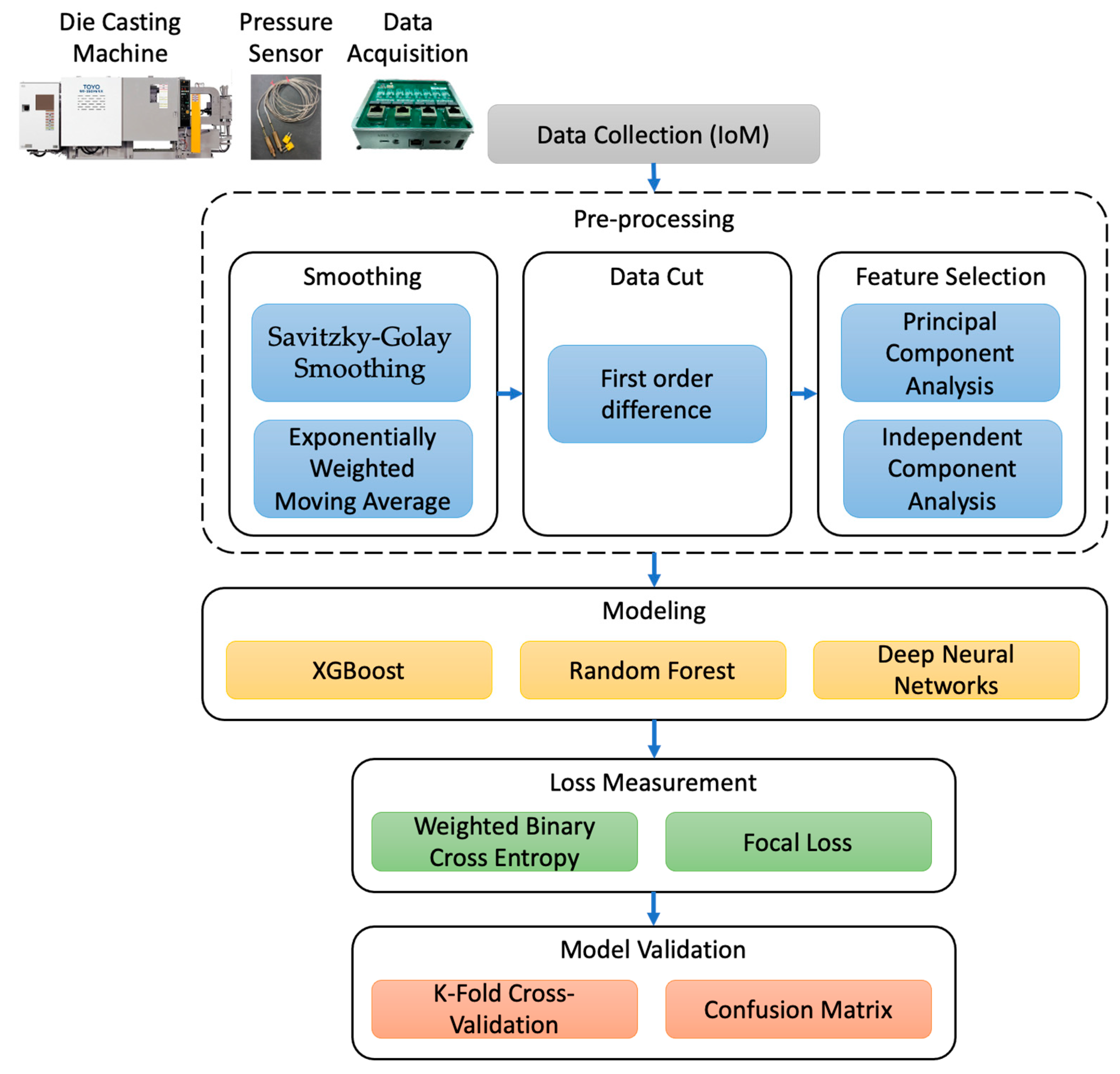
A pressure sensor is installed in the die-casting cavity to collect the actual pressure inside the mold in the manufacturing process. The data type is the continuous variation value of pressure in unit time. Many mechanisms are actuated simultaneously in the operation of a die casting machine, and so there is some noise. Therefore, for processing this type of data, the analysis is divided into three major parts in this study, including “data pre-processing”, “machine learning model”, and “model evaluation”, as shown in Figure 1. The data are smoothed by data pre-processing to remove noise, and the important features are extracted and maintained, so that the model can learn the important features. In terms of a machine learning model, an appropriate machine learning algorithm is selected to build a classification model. Finally, the model effect is measured by the loss function and evaluation index as the basis of model adjustment and processing method before improvement.

Figure 1.
Flow chart of research process.
2.1. Smoothing
The actual data are sometimes coupled with many external factors to generate noises, such as the noise of machine in operation or the noise resulting from external environmental factors. As the noise of signals is collected together with data, influencing the correctness and trend of data as well as the subsequent model effect, excess noise oscillation should be removed by data smoothing to enhance the generalization of a machine learning model.
2.1.1. Savitzky-Golay Smoothing Filter
Common data smoothing methods are mean filter and exponentially weighted moving averages. The main drawback of these two methods is that the overall trend of the curve cannot be considered, which may deflect the overall trend of the curve. Cao and Chen (2018) used the Savitzky-Golay Filter (SGF) for extraction and integration of spatial characteristics [9]. The SGF fits convolution by setting the moving window and using the least squares method to smooth the curve and calculates the derivatives of various orders of the smoothing curve.
If the data in a window are x[] where = −m, ⋯, 0, ⋯m and the range of value is 2 m + 1, the an th-order ( ≤ 2 m + 1) polynomial (1) is constructed in this range, using the least square method for data fitting:
The square error (2) of the datapoint after fitting and the original datapoint is calculated as:
In order to minimize the square error , the partial differential operation is performed for to make each partial derivative (3) equal to 0:
The unit impulse response equivalent to the FIR filter can be obtained after calculation, which is convolved to obtain the convolution coefficient. Thus, the equation after Savitzky-Golay smoothing is (4):
Here, is the smoothing coefficient of Savitzky-Golay and can be obtained by using the least squares fitting.
2.1.2. Exponentially Weighted Moving Average (EWMA)
Borror and Montgomery (1999) proposed the exponentially weighted moving average (EWMA) [10] for observing the trend of overall samples. Differing from SMA, EWMA can give different weights to the observed values, where present sample datapoints are given weights according to time. The nearer time point has a higher weight, the farther time point has a lower weight, and the overall moving average is obtained, so as to improve the high distortion of SMA. The EWMA equation is defined as (5):
We note that is the weighting constant with the range of , where the closer the value is to 1, the lower is the weight for the prior data. The initial value of is (when ), and sometimes the average value of overall data is used as the initial value; i.e., . The (CL) central line and control line can be constructed according to and sample , where . The control limit is:
In the part of pre-processing, the EWMA and Savitzky-Golay smooth denoising methods are used for smooth denoising of data. The effects of the two smoothing methods are then compared.
2.2. Data Cut
In machine learning, picking representative features out of the data can prevent the machine learning model from learning useless features, which influence the generalization of entire model and increase the learning efficiency of the model. Feature dimension reduction can lower the ineffective or incorrect features in high-dimensional data, so as to shorten the feature screening time and the model training time.
In terms of the first-order difference, when the data trend of a time series is unstable, the trend factor can be neutralized by differencing in order to stabilize the waveform. The first-order difference assumes in a discrete function that is the data of the -th time point, is the data previous to , and is the data of time points before . Thus, the subtraction of consecutive values is performed to obtain the difference; i.e., the definition of the first-order difference, which is:
2.3. Feature Selection
2.3.1. Principal Component Analysis (PCA)
Principal component analysis is a common technique for reducing data dimension and keeping the overall characteristics of data as much as possible. The basic assumption is to project the data into other low-dimensional spaces and to find out more typical main components [11]. The main practice is to find out a new axis of projection to project data again and to find out the principal component with the largest amount of data variation after projection. If the data sample set has data dimension of (8), then the reduced dimension is , and all samples are standardized as Equation (9):
The covariance matrix is then calculated as:
The eigenvector and eigenvalue are worked out by using singular value decomposition. The maximum eigenvalues and the corresponding eigenvectors are extracted to form a new matrix , where each sample is projected again and converted into a new sample . The new sample dataset is obtained by:
2.3.2. Independent Component Analysis (ICA)
Hyvärinen and Oja (2000) proposed the theory and application of ICA [12]. The main idea of ICA is derived from the known cocktail-party problem in psychology—namely, the cocktail effect. It explores how people can hear dialogues or voices they want to hear in a noisy cocktail-party environment. ICA is developed in statistics and assumes that the data on hand are mixed, with the expectation of deducing independent distributions from the data on hand. For example, when a microphone is used for sound reception, the source of audio is usually mixed with different sound sources, such as the host’s speech, others’ talking, and ambient background music. The speech can be separated from the background music or noise by ICA.
ICA linearly combines the original variables by projection. The generated components can maximize the explanation of the amount of variation of the original data, if a signal is a random vector with length of m as in:
This random vector is mixed with n signal sources and a noise to form:
Here, is the signal source; is the signal source mixing ratio; and is the noise. The expected value is usually assumed to be a normal distribution of 0. If A can be guessed, then can be worked out, and the clean signal source is restored by .
ICA has fast convergence speed and can be used in the data of non-gaussian distribution, but it has an overly long training time for data with a large number of features. The most important point is that ICA regards each feature as an independent attribute; this is different from PCA. PCA does not require the features to be independent attributes. The data features are pressure changes at different time points in this study. Not every feature can be regarded as an independent one. Thus, this study uses PCA to reduce the features of data and disregards ICA.
2.4. Classification Model
2.4.1. Extreme Gradient Boosting (XGBoost)
XGBoost was proposed by Chen and Guestrin [13] in 2016. Ogunleye and Wang employed the XGBoost model in the medical field for detection and prediction of chronic disease of the kidney [14]. XGBoost was improved based on the gradient boosted decision tree, and its core idea is to use each decision tree for prediction. First, a decision tree is built, and the residual between this decision tree and target answer is calculated. The second decision tree is then built to predict the residual, with the rest being deduced accordingly. The prediction values of all decision trees are added up at last, and the residual value to the answer is minimized. XGBoost can be regarded as a model of an ensemble tree.
If there are K decision trees as (14):
where the objective function is (15):
where is the loss function, calculating the difference between the predicted value and true value; is the regularizer of the model; T is the number of decision tree leaves; and is the weight of a leaf. The overall objective is to minimize the objective function.
XGBoost considers the parameter optimization problem of multiple trees, but we cannot train all the trees at one time. Thus, additive training is used, where the original model remains after each optimization, and the prediction of this tree is provided, leading to:
The objective function can be expressed as (18):
The second-order Taylor expansion is performed for the loss function in position to obtain (18):
where:
and the constant term is removed as:
We define as No. j leaf point, and then get:
To minimize the objective function, let the derivative be 0, as in (23):
This optimum solution is substituted in the objective function to obtain (24):
2.4.2. Random Forest
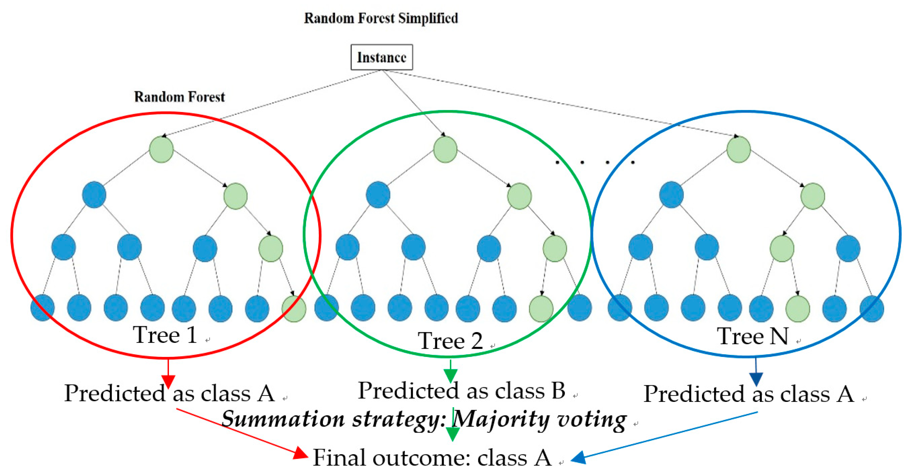
Random forest is a combinational algorithm proposed by Breiman in 2001, which uses multiple decision trees as the basic classifier for prediction [15]. Katuwal et al. used the random forest algorithm in medicine in 2020 [16]. First, the decision tree is a tree-based prediction model composed of nodes and directed edges. The tree structure comprises root nodes, branch nodes, and leaf nodes. The parameter of each node of a decision tree is not selected in all parameter spaces, but randomly selected in a fixed quantity of parameter spaces. The random forest leads dual randomness in the instances and parameters to guarantee the diversity of the generated basic classifier. The best splitting point is selected in a random subspace when building the decision tree, but the calculation of an optimum attribute is not random. However, when following a certain attribute selection principle, the accuracy of the basic classifier is guaranteed to some extent. The algorithms include ID3, C4.5, and CART. The random forest proposed by Breiman uses the classification and regression tree (CART) of decision trees.
In the construction process of a decision tree, each leaf node of the tree selects the “important” parameters from numerous parameters according to a certain principle. As the random forest is the integration of decision trees, it inherits the ability of the decision tree to select important parameters. The difference is that the random forest uses an implicit method for parameter selection. When an important parameter has noise, the accuracy of prediction is supposed to decrease obviously. If this parameter is an uncorrelated parameter, the influence of the noise on the prediction accuracy may be slight. Based on this idea, when out-of-bag data are used to predict the random forest performance, then in order to know the importance of a parameter, the value of the parameter is modified randomly, and the other parameters remain. The importance of the parameter is learned from the difference between the out-of-bag data prediction accuracy and the original out-of-bag data prediction accuracy.
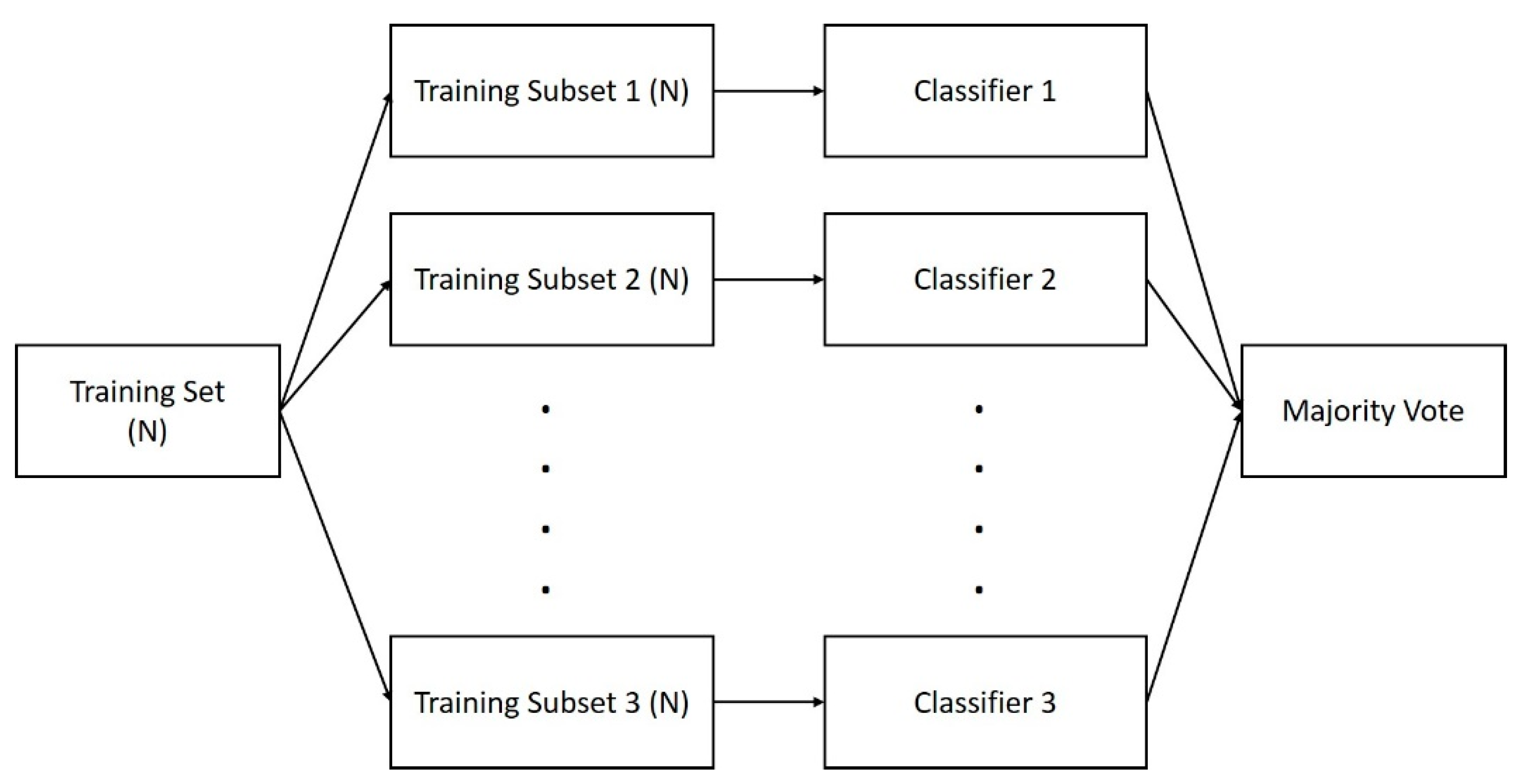
The random forest algorithm uses ensemble learning, and multiple classifiers are built by using the bagging (bootstrap aggregation) sampling method, as shown in Figure 2. Here, n samples are randomly extracted from the original training set N for training (n < N) and restored after extraction to train n classifiers. Each classifier obtains the final prediction result by voting. The random forest uses bagging to extract the training subset on the same scale for each CART tree from the original training set and introduces a randomly selected attribute into splitting each node of the CART tree, so that the correlation between trees is reduced. The established single unpruned decision tree can guarantee lower deviation to guarantee the classification performance of the random forest. The overall architecture of the random forest is shown in Figure 3.
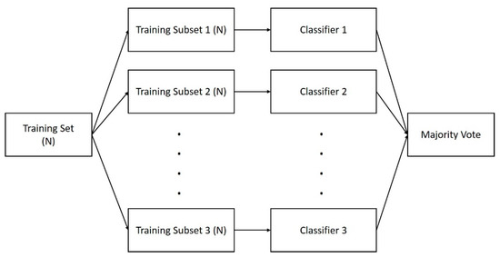
Figure 2.
Bagging diagram of an integrated algorithm.

Figure 3.
Random forest structure diagram.
2.4.3. Deep Neural Networks (DNN)
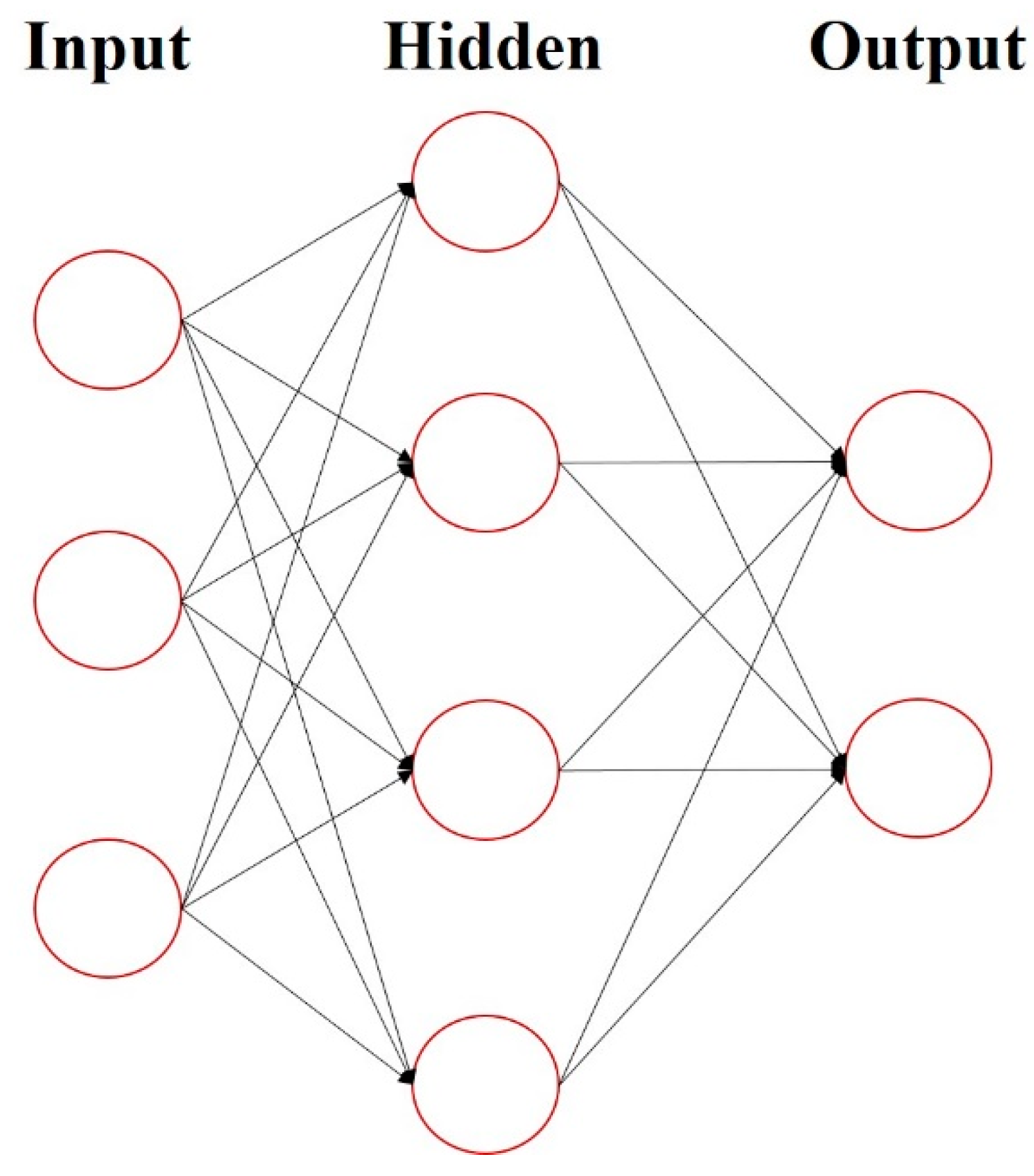
Artificial neural network (ANN) is a mathematical model created by imitating the human central nervous system (such as the brain structure with functions), which simulates the signal transmission process through an electric current of synapses by the neurons in the brain. The signal transmission depends on the signal magnitude received by the neuron cells. When the signal magnitude exceeds a threshold, the current is given and transmitted to the next neuron through the synapse, and so ANN simulates the signal transmission process of the brain. Abiodun and Jantan (2018) reintroduced the classic model and its application [17]. Lin et al. (2020) applied DNN to identify the threat of adversarial attack [18].
The architecture of an artificial neural network is a neural network architecture with one input layer, one output layer, and at least one hidden layer, as shown in Figure 4. Each neuron has a weight to decide whether or not to transfer the message to the next layer. Simply put, the neural network learns how to update the weight on each neuron to find the best prediction result.
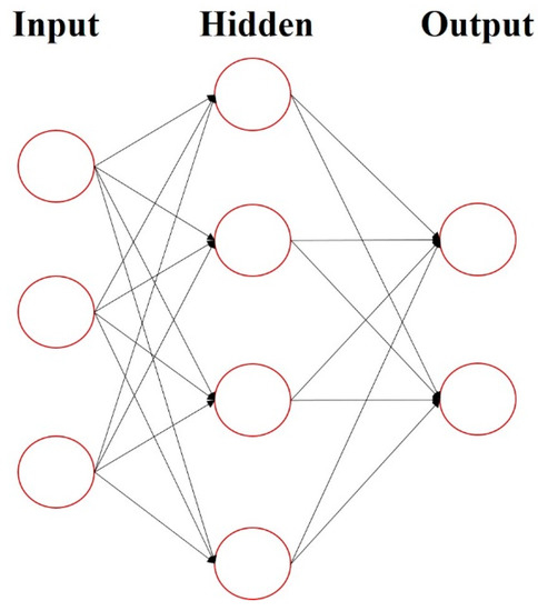
Figure 4.
Artificial neural network (ANN).
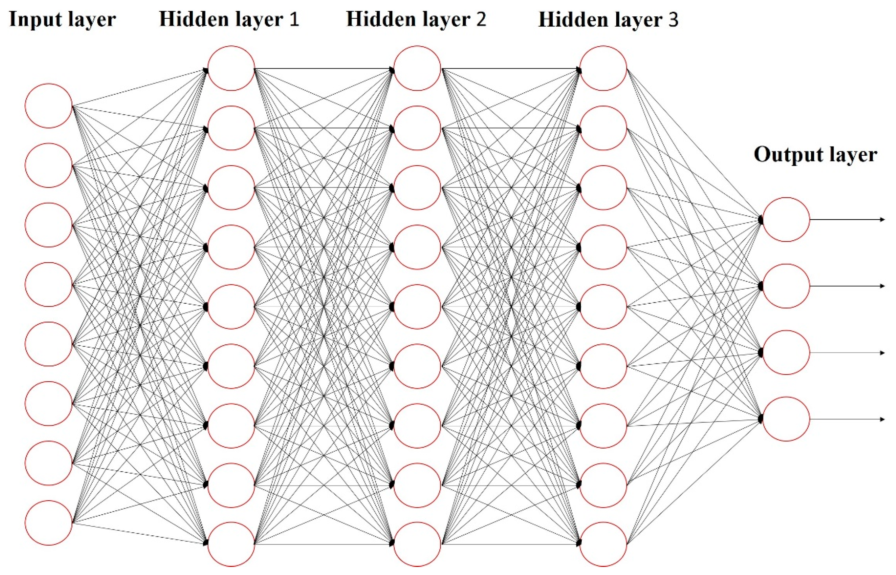
DNN increases the quantity of hidden layers of ANN and enhances the model training effect. Thus, it is also known as multilayer perceptron (MLP), as shown in Figure 5.
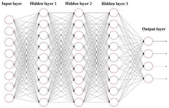
Figure 5.
Deep neural network, DNN.
Sze and Chen used DNN to build a complex non-linear system model, the back propagation algorithm for training, and used partial differentiation and the chain rule to correct the weight and threshold of MLP [19], as expressed in Equation (25):
Here, is the adjustment of the weight between the th neuron of the layer and the th neuron of the previous layer calculated by using the th data; is the learning rate; is the value of the th neuron of the previous layer of the th data; and is the local gradient value of the th neuron of the layer calculated by using the th data. Therefore, the calculation approaches corresponding to whether the layer is an output layer are different; if the layer is not output layer, then the chain rule should be used for calculation.
There are many methods for optimizing and correcting weights, besides the said backpropagation algorithm, such as Momentum, Adagrad, Adadelta, and RMSprop. The common method is Adaptive Moment Estimation (Adam), which is an optimization algorithm combined with the concepts of Momentum and Adagrad.
The weight update is computed by using Stochastic Gradient Descent (SGD), expressed as Equation (26):
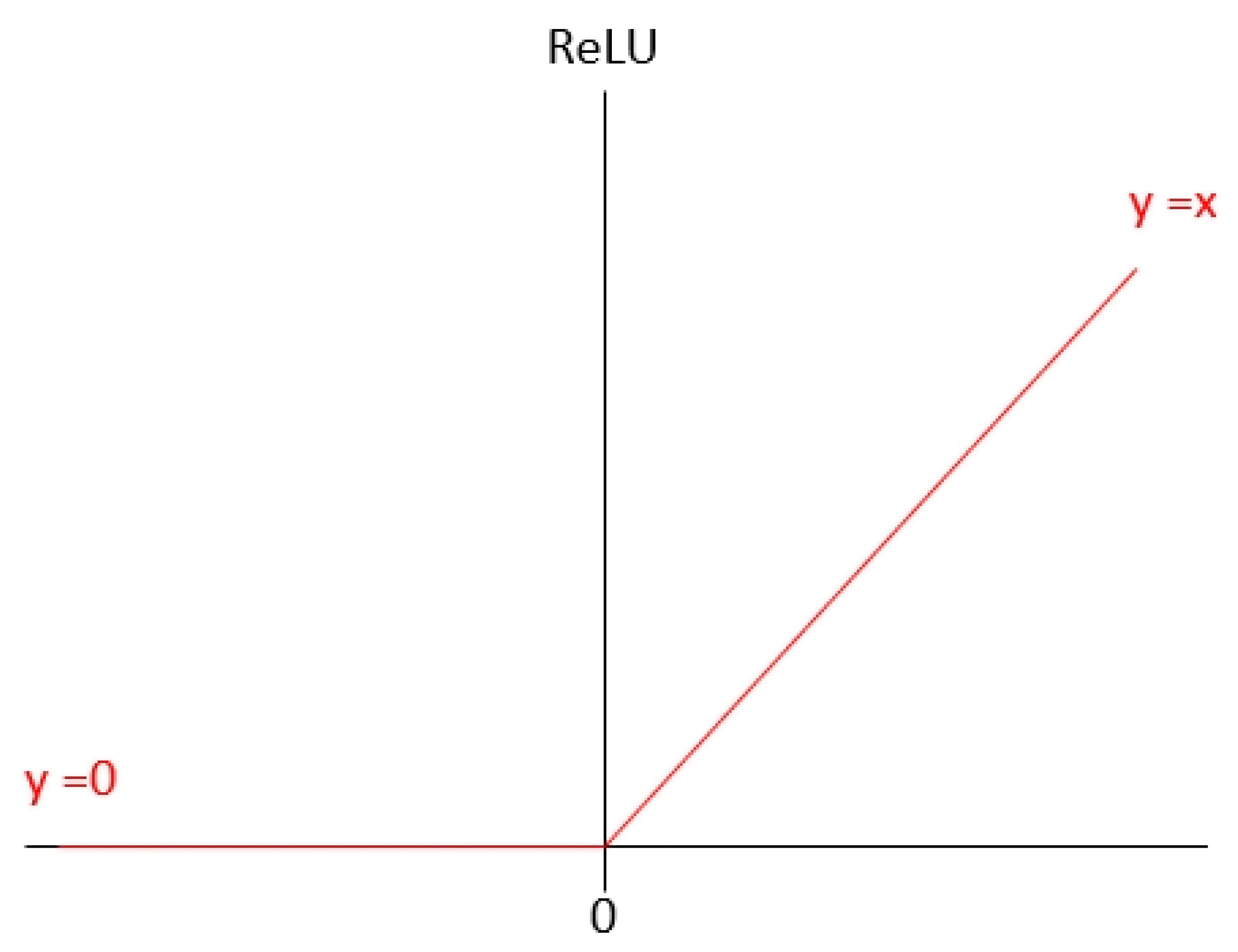
Here, η is the learning rate; and C is the loss function. The selection of loss function is related to the learning problem (e.g., classification problem and regression problem), learning method (e.g., supervised learning, unsupervised learning, and reinforcement learning), and selection of activation function (ReLU, Leaky ReLU, and Softmax). The activation function uses a non-linear equation to solve a non-linear problem and to solve the vanishing gradient problem and exploding gradient problem in the process of back propagation. ReLU is shown in Figure 6, which is the most frequently used activation function, expressed as Equation (27):

Figure 6.
Loss function ReLU.
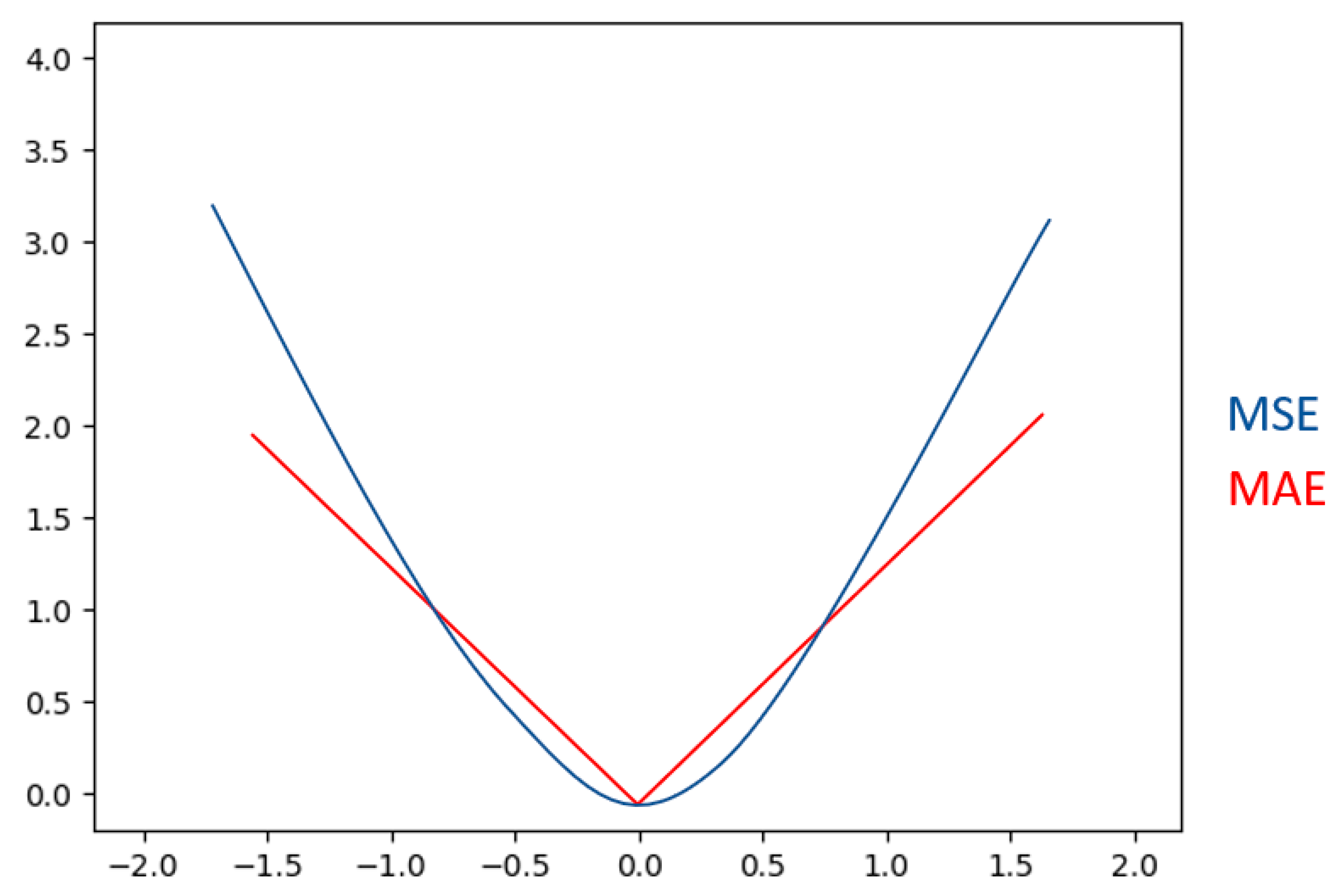
The common loss functions include Mean Square Error (MSE) (28) and Mean Absolute Error (MAE) (29) for the regression problem, expressed as follows:
Here, n is the amount of data; is the predicted value; and y is the true value. The difference between MSE and MAE is shown in Figure 7.
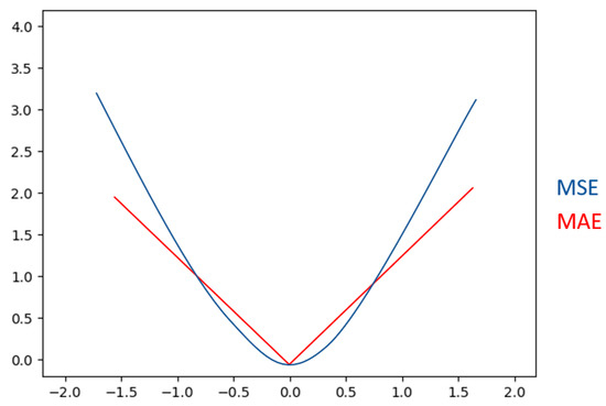
Figure 7.
Difference between MSE and MAE.
The classification problem is usually defined by Cross Entropy H as (30):
Here, C is the number of classes; n is the total amount of data; is the true class corresponding to One Hot Encode; and is the probability of belonging to class of data after prediction.
The most frequently used activation functions for output layer are Softmax and Sigmoid. Softmax is expressed as Equation (31):
Here, is the probability of belonging to class ; and and are the input to units and , respectively.
The definition of Sigmoid, Equation (32), is shown in Figure 8:
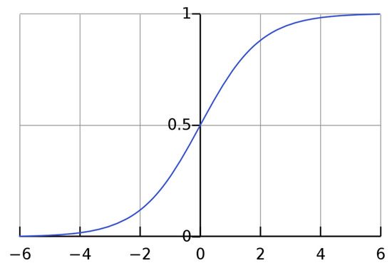
Figure 8.
Sigmoid curve.
2.5. Loss Function
In machine learning the loss function can help the model correct errors in the process of learning, so as to enhance the generalization degree of the model. The ultimate objective of the model is to minimize the loss function, and so the loss function can be described as an objective function. The loss function helps the learning of the model as well as the learning weight of the model for positive and negative samples in the case of sample imbalance by different designs.
2.5.1. Weighted Binary Cross Entropy
Cross entropy is a classic loss function in the domain of deep learning. Boer and Kroese (2005) introduced the cross entropy loss function algorithm and the principle in detail [20]. In the scenario of data imbalance, the learning of the model for minority class samples can be enhanced by modifying the cross entropy sample weight. Because cross entropy represents the importance of a sample for loss, the contribution of minority class samples can be increased by increasing the weight of minority class samples, defined as Equation (33):
Here, is the th data; is the actual label class of the th data; is the model predicted probability; and is the weight adjustment for positive class samples. According to Equation (10) above, the weighted binary cross entropy adjusts the weight for positive class samples and enhances the learning of the model for positive class samples. Thus, the minority class sample is usually defined as a positive sample in design.
2.5.2. Focal Loss
Lin and Goyal (2017) proposed the focal loss function [21]. Qiao and Bae et al. (2021) used focal loss to build an integrated neural network to detect COVID-19 [22]. Focal loss improves the traditional cross entropy and improves the failure in learning the difficulty level of samples. Cross entropy is defined as Equation (34):
Here, is two different classes of samples of −1 and 1; and is the probability of some class of sample predicted by model, with the value of 0~1. We rewrite as in Equation (35):
Therefore, the cross entropy equation can be rewritten as . For an unbalanced sample, the CE loss function is multiplied by an weight for adjustment, and the sample lacking confidence is given a larger weight, as expressed in Equation (36):
As stated above, the unbalanced positive and negative samples can be modified by using weighting parameter α, but the difficulty level cannot be learned. Hence, the weighting parameter is modified to , distinguished as a modulating factor, and focal loss is defined as Equation (37):
Here, .
When the sample is misclassified, Pt is a small value, and the modulating factor approaches 1. At this point, the influence of the loss function is slight in general. However, when the sample is classified correctly, Pt has a value close to 1, the modulating factor approximates 0, and the classifiable sample weight decreases greatly. The parameter r is further modified for the modulating factor, and the proportion of simple sample learning can be adjusted. When r = 0, FL is equivalent to CE; in a direct view, the modulating factor greatly reduces the easily classified sample weight of the model, so that the model can further focus on the samples that are hard to be classified.
2.6. Model Evaluation Index
Model evaluation is very important in the domain of machine learning. Pre-processing modification, model improvement, and problem detection can be implemented according to the evaluation result. After the most traditional evaluation method is to classify the data into a training set, validation set, and test set, the model is then modified by using the validation set, and the test set is used as the final model effect. However, the major defect in this method is that the data partitioning result changes every time, it is difficult to achieve objectivity, and so K-fold cross-validation occurs. The model can learn each condition to the maximum content and perform efficient modification and improvement.
2.6.1. K-Fold Cross-Validation
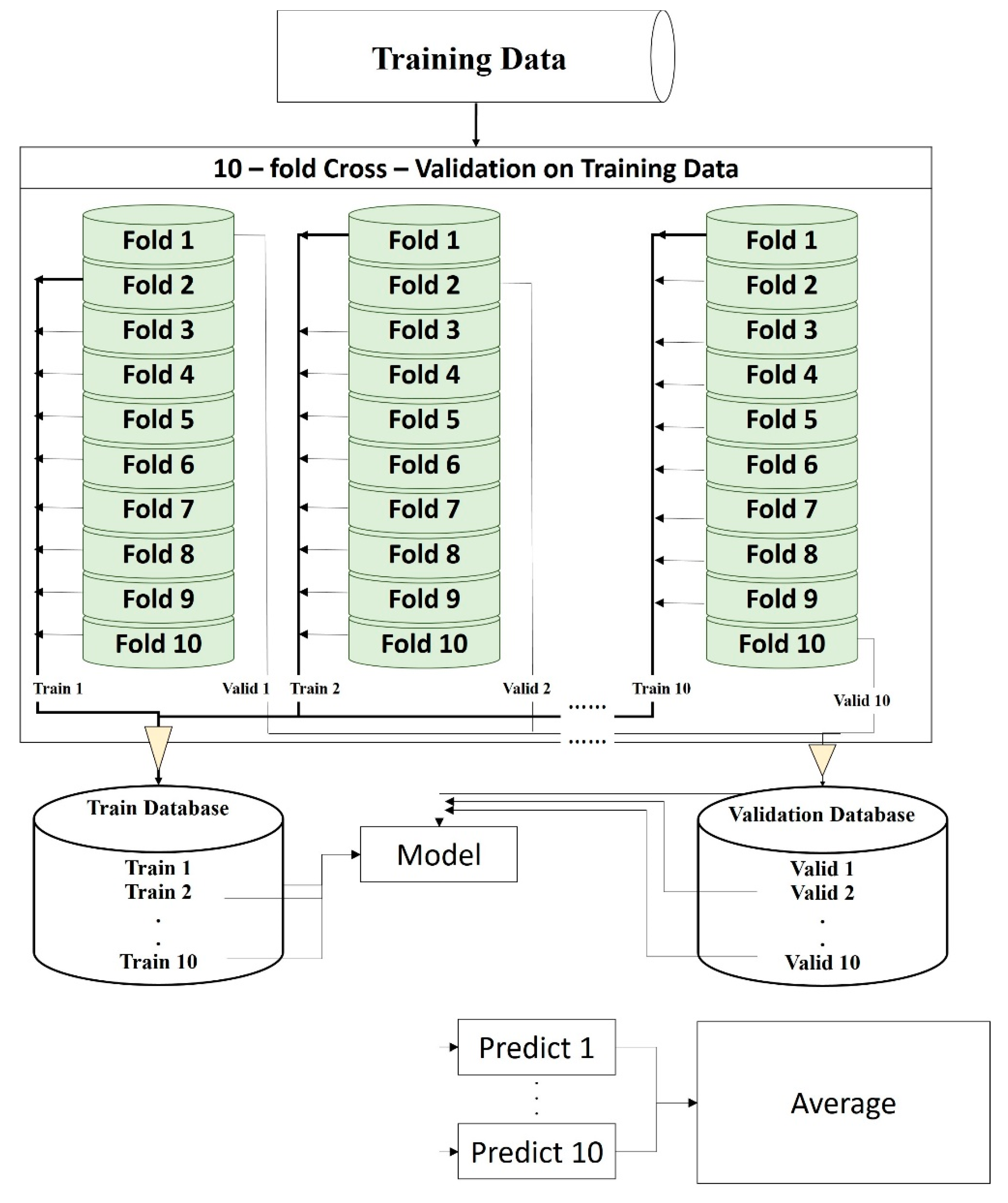
Cross-validation is a method for testing the fitness of the model. It can effectively validate whether a model is overfitting or underfitting and check the effect of the entire model. It divides the dataset into K parts of data for cross-validation. One part is taken as validation data in each training process, the other K-1 parts are used as training data, and the result is predicted. Other validation data re used for the second training, and last validation data are returned to the training dataset, guaranteeing 1 part of validation data and K-1 parts of training data for each training, until all the partitioned data are used as a validation set. The overall training process is thus performed K times. Finally, the K training results are averaged, and the result is used for evaluating the overall effect of model. The process is shown in Figure 9.
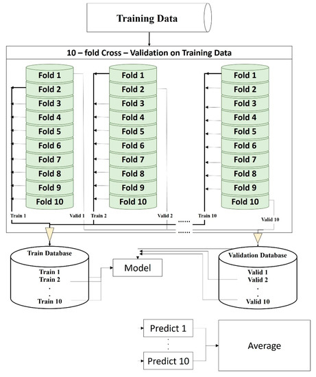
Figure 9.
K-fold cross-validation flow chart.
2.6.2. Confusion Matrix
In machine learning the confusion matrix is most frequently used to evaluate the model performance in a classification problem. The confusion matrix has four major elements as shown in Table 1: Tp (True Positive), Tn (True Negative), Fp (False Positive), and FN (False Negative). The four major elements are defined as follows.

Table 1.
Confusion Matrix.
- Tp (True Positive): the true value is Positive, the predicted value is Positive.
- Tn (True Negative): the true value is Negative, the predicted value is Negative.
- Fn (False Negative): the true value is Positive, the predicted value is Negative.
- Fp (False Positive): the true value is Negative, the predicted value is Positive.
To measure the model effect, accuracy, precision, recall, and F1 Score measurement indices of the model calculated by the four major elements, the computing equations (38) are:
3. Results
3.1. Data Description
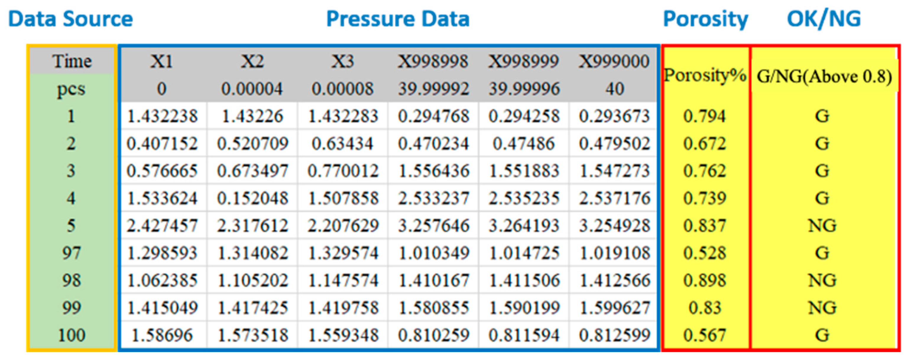
The pressure variation inside the mold in the casting process is collected by the sensor. The production cycle time of each cast is 40 s, and the sampling interval is 0.00004 s. There are 100 data observations collected, and each one has 999,000 datapoints, each of which shows the pressure value of each datapoint at each time point. The last two columns show the porosity and product quality of various data. Porosity higher than 0.8 is identified as NG product. It is a structured data type. The data structure is shown in Figure 10.
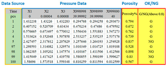
Figure 10.
Press casting data structure.
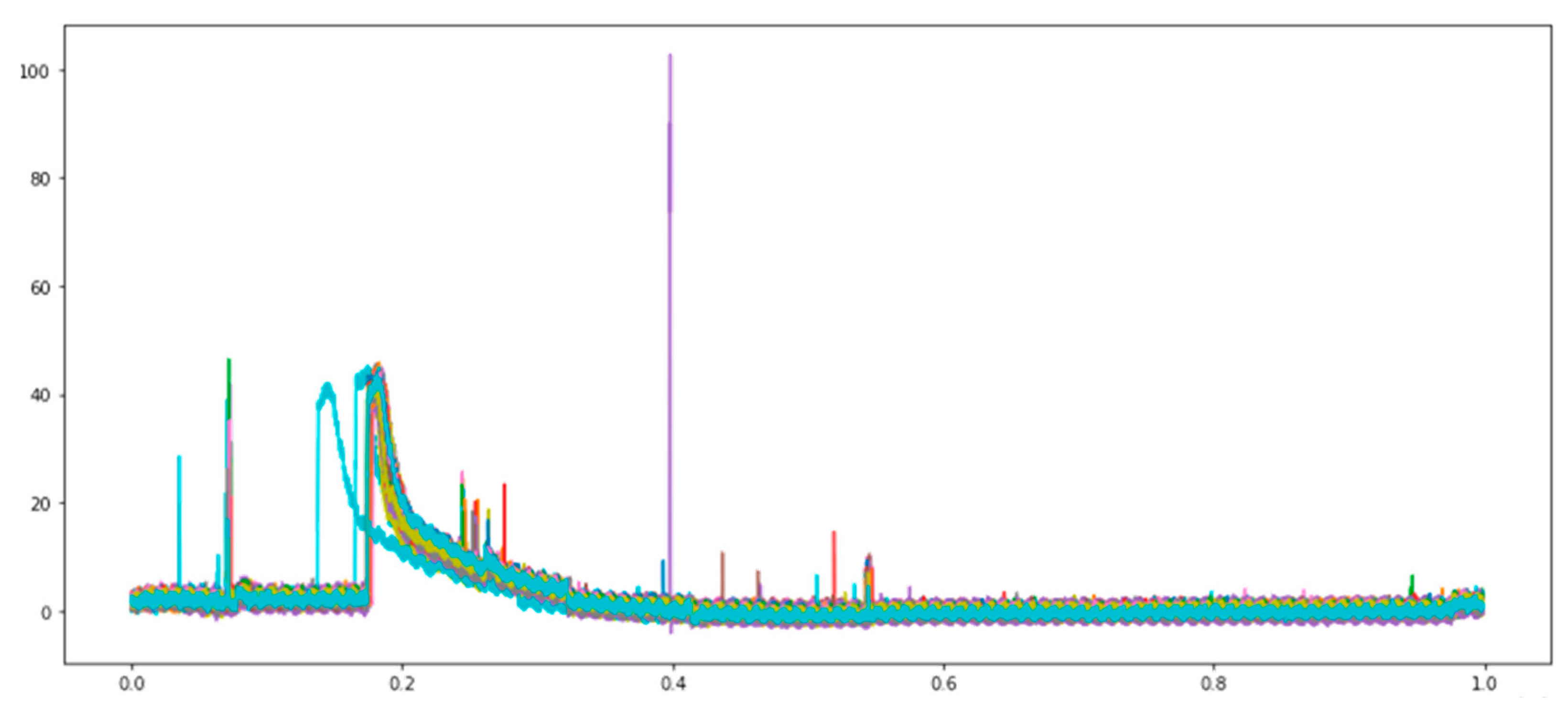
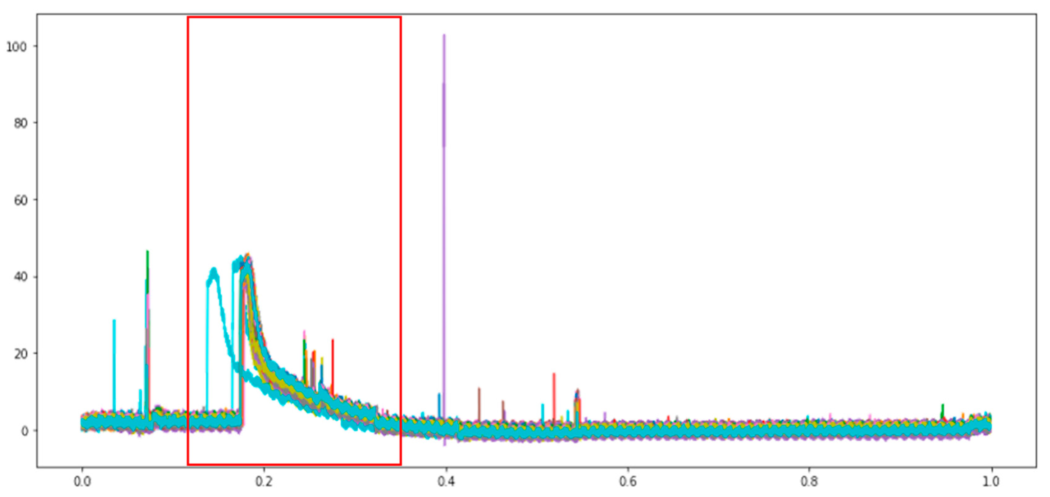
The curve of 100 pressure data is then drawn. The data characteristics are observed graphically, and the available data pre-processing mode is analyzed. The pressure curve changes are shown in Figure 11.
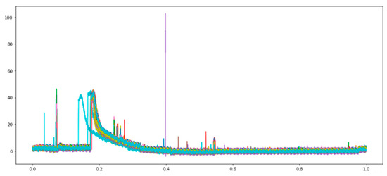
Figure 11.
Graph of pressure curve variation.
The data contain a lot of noises, and several data are offset in the course of collection. The excess noise should be filtered, and the useful features are maintained, meaning only the pressure variation in the period of injecting high pressure into the mold is maintained, as shown in Figure 12 (red frame). As the other features are the noises of machine operation in the data gathering process, these noises are useless information for the model can could influence the effect of subsequent model training. The offset of data is a major problem to the model, as it makes various data lose their reference points, thus influencing their effect. The SGF and EWMA are used for smooth denoising. The two smoothing effects are compared, and the best smoothing effect is selected. The problem of data offset is solved by using the first-order difference.
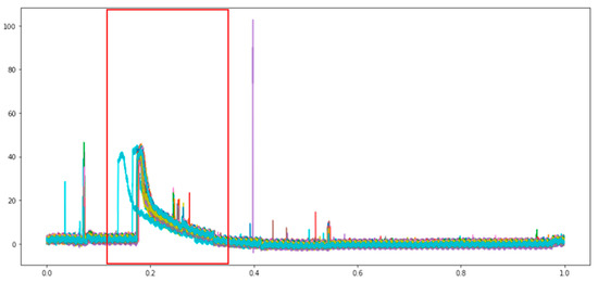
Figure 12.
Feature retention range(Red frame).
3.2. Data Smoothing
For numerical data, the common smoothing methods include Exponential Smoothing (ES), the Exponentially Weighted Moving Average (EWMA) proposed by C. M. Borror, D. C. Montgomery & G. C. Runger in 1999 for enhancing the smoothing effect of control sheet, and the SGF smoothing based on the said two methods published by R. W. Schafer in IEEE in 2011. Besides setting the sliding window size, the SGF smoothing uses the least squares method and uses a polynomial to fit the data in the sliding window for smoothing. The original appearance of waveform is maintained as much as possible, and the loss of useful information after smoothing is reduced. This study employs EWMA and SGF smoothing methods and compares the effects of the two methods on in-mold pressure data and their merits and demerits to select the optimum smoothing method.
3.2.1. EWMA Smoothing Effect
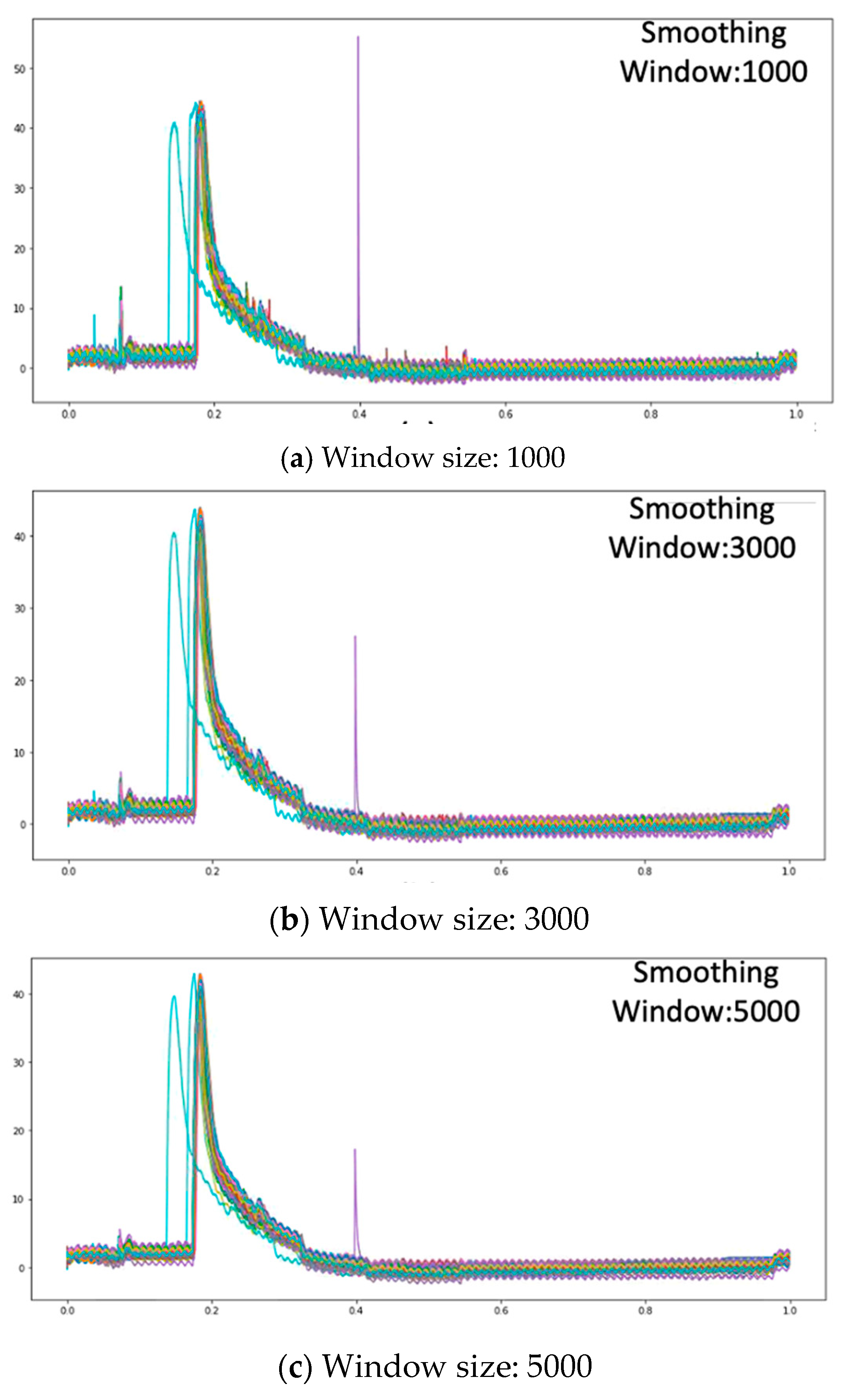
EWMA is a very conventional tool for statistical data processing in the domains of finance and management, for observing the trend of data waveform. It is used for data smoothing in this paper, and varying degrees of smoothing are performed by adjusting the size of smoothing window. As the collected data feature points are large, the values should not be too small in the parameter setting of the EWMA sliding window. According to experimental results, three sliding window sizes are compared: each interval is 2000, and the sizes are 1000, 3000, and 5000. If the smoothing window is smaller than 1000, then the smoothing effect is poor. If the size is larger than 5000, then the smoothing is excessive, and the waveform is distorted severely. The EWMA smoothing window settings and smoothing effects are shown in Figure 13.
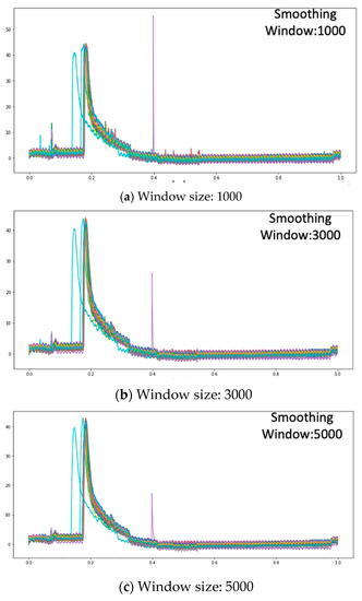
Figure 13.
Comparison of EWMA smoothing effect by different window size.
Low noise can be filtered out when the smoothing window is set as 1000, but the effect on high noise is not ideal, as shown in Figure 13a. When the smoothing window size is set as 3000, high noise cannot be processed, as shown in Figure 13b. Finally, when the smoothing window size is 5000, the smoothing effect is better, partial noise can be eliminated, and the excessive noise effect can be reduced, as shown in Figure 13c. However, the sliding window should not be too large; if the sliding window is too large, the features are lost as the overall curve is too smooth, leading to severe offset.
3.2.2. SG Filter Smoothing Effect
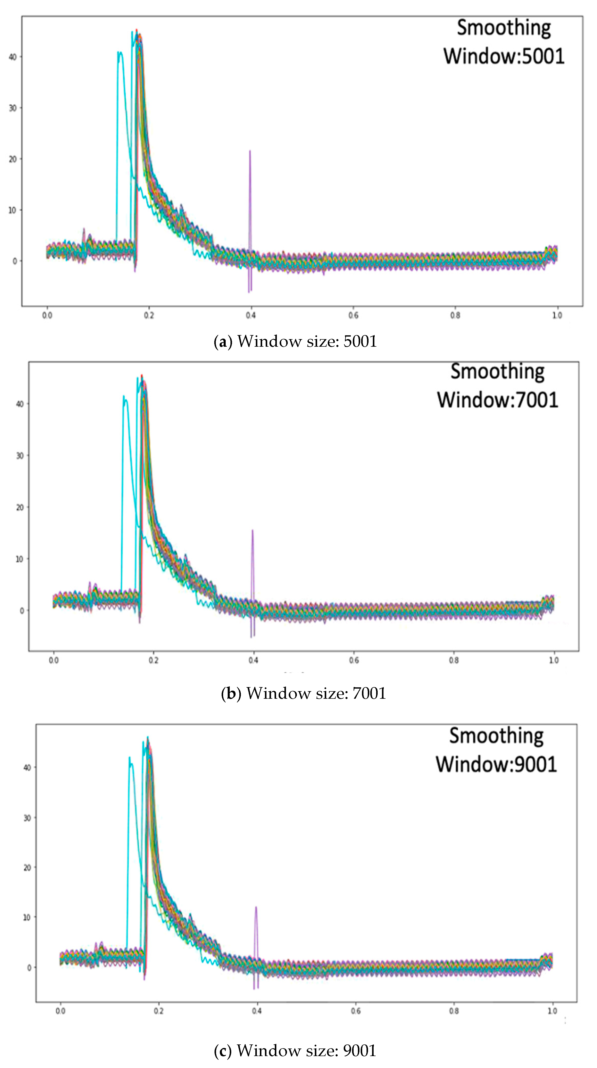
Compared to EWMA smoothing, the SGF maintains the complete characteristic of the waveform better, as it uses the least squares method for fitting in each window and can set the maximum power of this fitting equation to represent the complexity of the equation. Therefore, the SGF has higher reduction degree of original data than EWMA. When the sliding window is large, the SGF not only eliminates more noises, but also maintains the integrity of the waveform as best as possible, achieving a dual effect. Generally, in the setting of the SGF fitting equation, the maximum power is set as the third power, and so the effects of three smoothing window sizes on noise filtering and waveform distortion degrees are compared by setting the maximum fitting power as the third power. The smoothing window sizes are 5001, 7001, and 9001. The effects are shown in Figure 14.
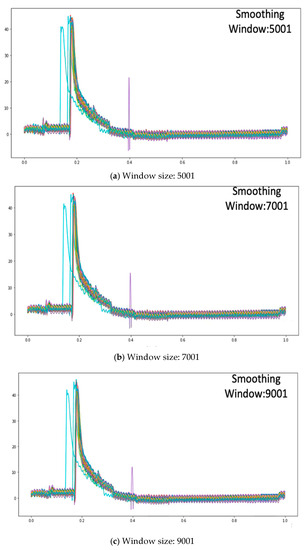
Figure 14.
Comparison of Savitzky-Golay Filter smoothing effect by different window size.
According to Figure 14, most noise can be filtered when the smoothing window size is 5001, and the filtering of high noise is acceptable, as shown in Figure 14a. High noise can be filtered out more efficiently without waveform distortion when the smoothing window size is set as 7001, as shown in Figure 14b. Therefore, the smoothing effect is better when the smoothing window size is set as 9001, as partial noise can be eliminated to reduce any excessive noise effect. However, the waveform is distorted if the smoothing window is too large, and so the best SGF smoothing window is 9001.
3.3. Data Alignment
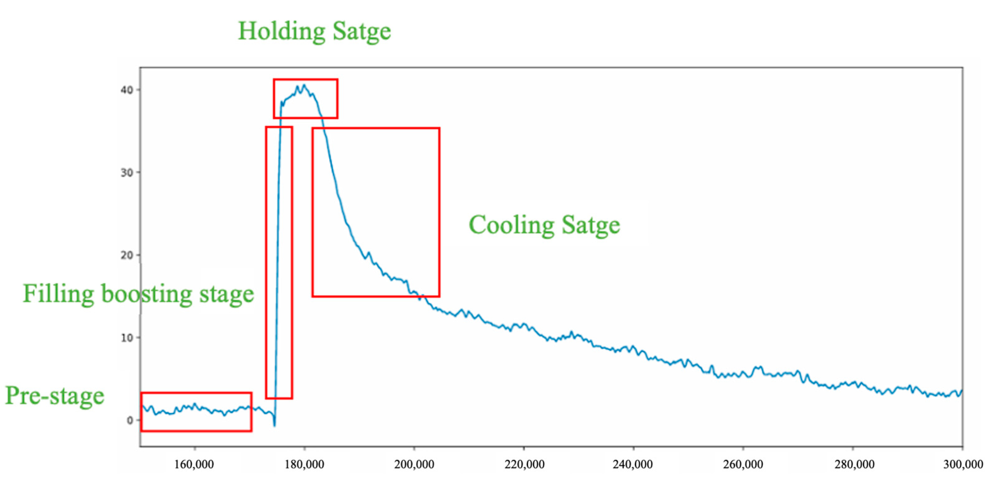
The press casting process is approximately divided into pre-stage, filling boosting stage, packing stage, and cooling stage, as shown in Figure 15. The in-mold pressure stability is the key to product quality, and so each stage may be the quality influencing factor.

Figure 15.
Various stages of casting.
The packing stage is therefore the key time point that influences non-defective and defective products. However, due to the time difference in the course of data collection, the data have a time offset. In order to highlight the difference between non-defective and defective in the packing stage and cooling stage as well as to guarantee the reference point of comparison, the start points of various data should be aligned to avoid the influence of time offset. Therefore, the first-order difference is used to look for the alignment point to solve the data time offset.
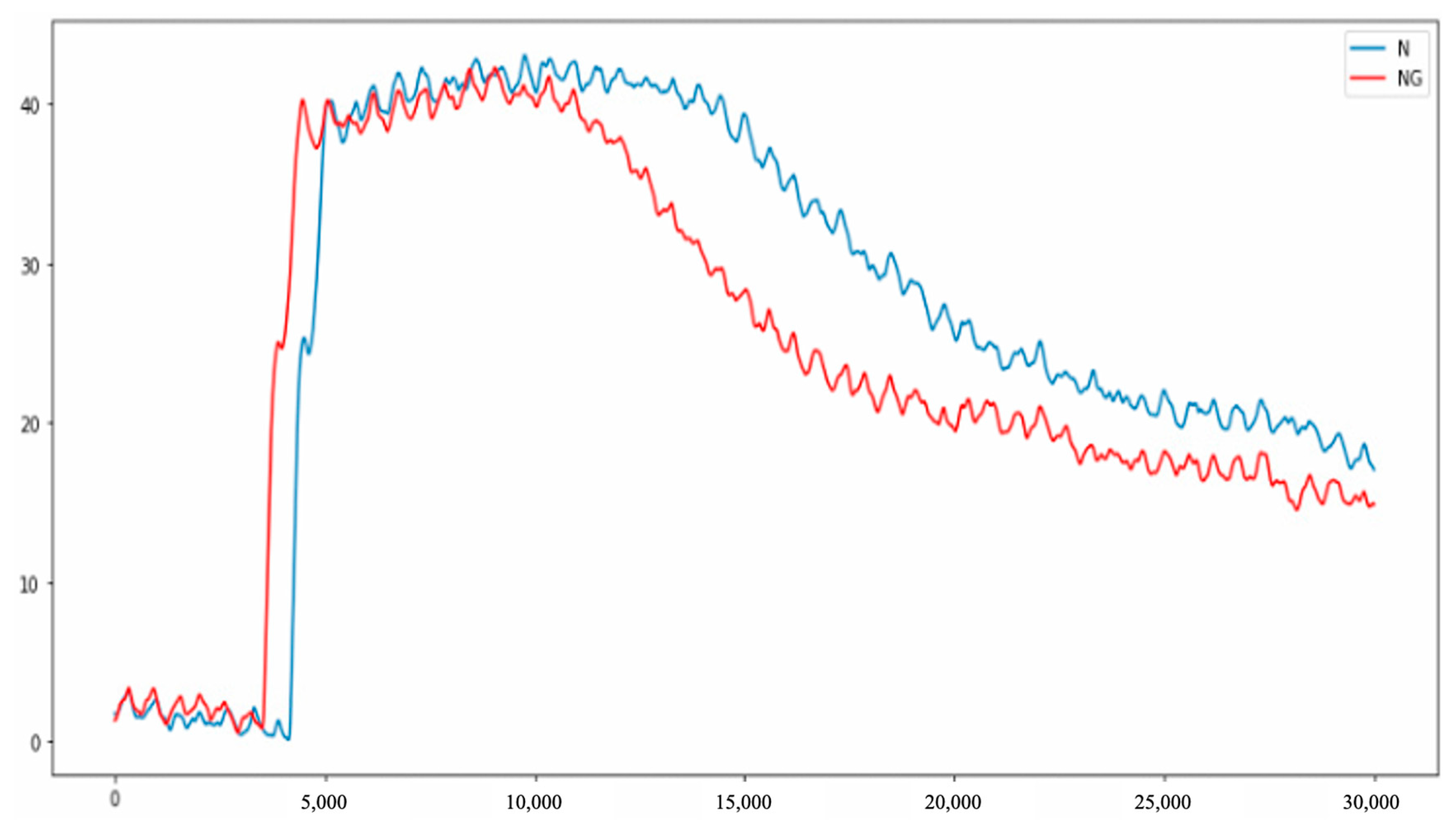
According to the pressure variations of defective and non-defective in the said stages, the duration of pressure variation of defective in the packing stage is obviously shorter than the duration of non-defective. The pressure drops rapidly in the cooling stage, as shown in Figure 16.
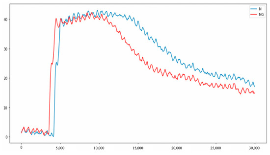
Figure 16.
Pressure curve difference between non-defective and defective.
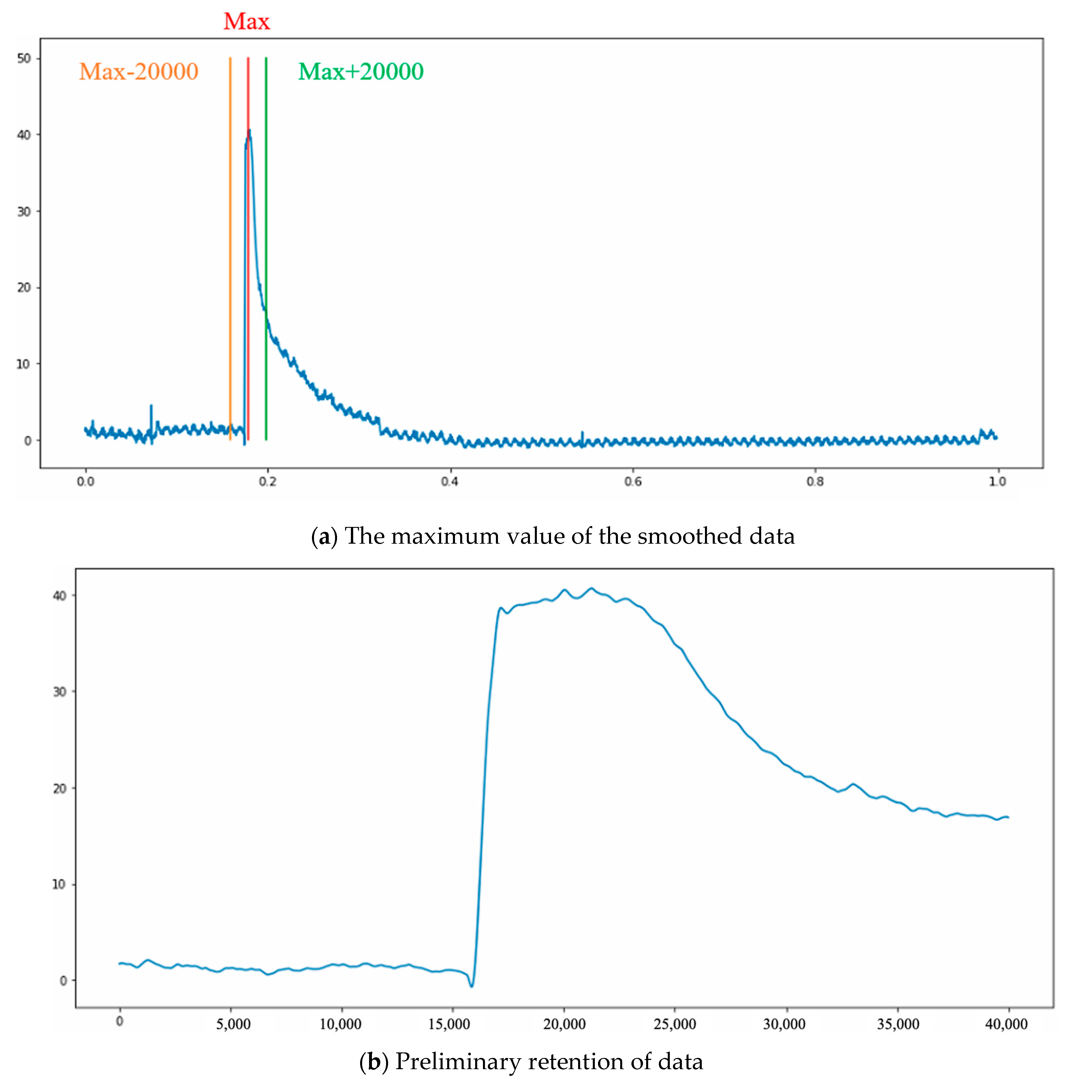
The time point of the rapid drop is used as the start point location of each data observation. To avoid waveform distortion and the other machine noises influencing the finding of the locating point, the maximum value of the smoothed data is used as a reference point, and the data of 20,000 feature points before and after the reference point are preliminarily maintained. The noise effect of the other segments is reduced without waveform distortion. The data of 40,000 points are maintained, as shown in Figure 17a, and the extracted graph is shown in Figure 17b.
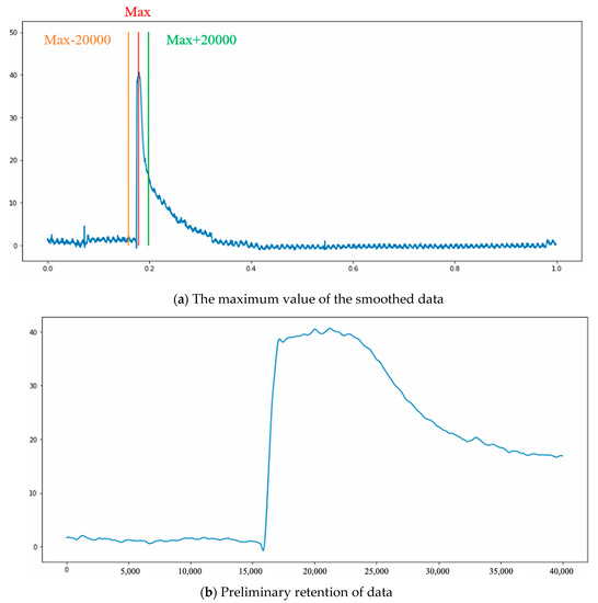
Figure 17.
Data area.
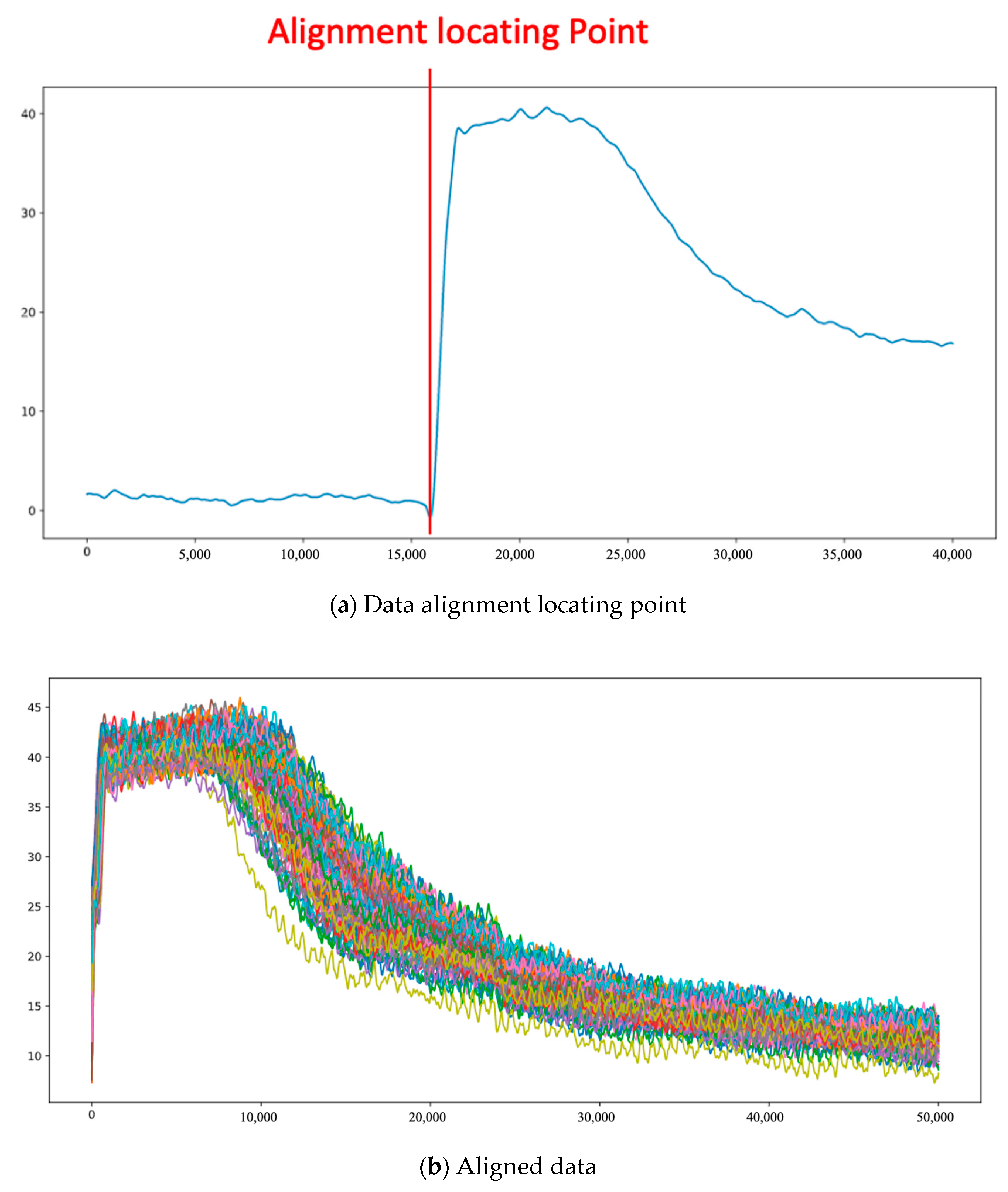
After preliminary range selection, the part for data processing can be maintained. The amount of computation and errors resulting from the other datapoints are reduced. For the preliminarily reserved feature pattern, the locating point of each data observation is obtained by using the first-order difference. The pressure difference between the next time point and current time point is calculated by using the characteristic of the first-order difference. When the pressure value at the moment and the pressure value at the next time point have the maximum difference, the locating point can be found, as shown in Figure 18a.
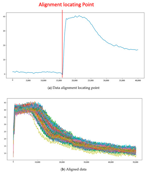
Figure 18.
Data alignment by first-order difference.
The said procedure is repeated, and after the locating points of data are found out, the start points of all data can be aligned in order to solve the time offset of data in the collection process, up to the cooling stage of the casting process after the data locating points. The data feature points are further reduced. The data of 999,000 feature points can be reduced to the data of 50,000 feature points. The aligned data appear in Figure 18b.
3.4. Data Dimension Reduction
This study uses principal component analysis (PCA) for data dimension reduction. The percent reduction is set as 99%, and the characteristics of data are restored as much as possible. The feature in a data feature size of 50,000 is converted into 20 principal features when the cumulative interpretation rate is 99%, and PCA features above 0.9 are selected. There are 17 features maintained at last as subsequent model input, and the prediction effects of using PCA and not using PCA are compared in subsequent findings. The cumulative interpretation is shown in Table 2.
Table 2.
PCA cumulative interpretation rate.
3.5. Modeling
3.5.1. DNN
In the setting of DNN, this study uses two hidden layers; in principle, the larger the number of hidden layers is, the better is the effect. Excessive hidden layers result in gradient vanishing and gradient explosion, increasing the training difficulty, and the model becomes difficult to converge. Thus, the number of hidden layers should not be increased infinitely. Two hidden layers are enough in general, especially when the amount of data is relatively small, as excessive hidden layers are likely to induce overfitting. In the setting of the number of neurons, too small a number of neurons induces underfitting of the model, and so this study uses two hidden layers and compares different loss functions, which are weighted binary cross entropy and focal loss. Different numbers of neurons are set up with different loss functions and combined with different pre-processing methods to observe the model effect. Lastly, the effects of the two loss functions are compared.
Weighted Binary Cross Entropy
The loss function of DNN uses weighted binary cross entropy to adjust the weight of the minority class sample. The numbers of neurons are 32, 16, and 8 for permutation and combination. EWMA smoothing is used to compare the model effects with and without PCA. When PCA is not used, the numbers of neurons of hidden layer are 16 and 8, and the effect is the best, with accuracy of 85%, precision of 50%, and recall of 73.33%.
The SGF smoothing is used next. The model effects with and without PCA are compared. The numbers of neurons of hidden layer are 16 and 8, and the effect is the best, with accuracy of 87%, precision of 55%, and recall of 73.33%, as shown in Table 3.
Table 3.
Weighted binary cross entropy.
According to a comparison, when EWMA or SGF is used for smoothing, the effect without PCA is better than the effect with PCA, and the SGF performs better than EWMA smoothing. Therefore, when the weighted binary cross entropy is used as a loss function, applying SGF smoothing without PCA can achieve the best pre-processing effect.
Focal Loss
The loss function of DNN selects focal loss as the loss function of the model. The weight of the minority class sample is adjusted, and the numbers of neurons are 32, 16, and 8 for permutation and combination. EWMA smoothing is used to compare the effects of the model with and without PCA. When PCA is not used and the hidden layer has 32 and 16 neurons respectively, the effect is the best, with accuracy of 87%, precision of 54.55%, and recall of 80%.
The SGF smoothing is now used, and the effects of the model with and without PCA are compared. When PCA is not used and the hidden layer has 32 and 16 neurons respectively, the effect is the best, with accuracy of 92%, precision of 73.33%, and recall of 73.33%, as shown in Table 4.
Table 4.
Focal loss.
According to comparison, when EWMA or SGF is used for smoothing, the effect without PCA is better than the effect with PCA, and the SGF performs better than EWMA smoothing. Therefore, when focal loss is used as a loss function, applying SGF smoothing without PCA can achieve the best pre-processing effect.
Comparison
The best pre-processing methods of focal loss and weighted binary cross entropy are now compared. The effects and confusion matrix are shown in Table 5. When focal loss or weighted binary cross entropy is used, the recall is 73.33%. However, the accuracy and precision of focal loss are 92.00% and 73.33%, respectively, or higher than 87.00% and 55.00 of weighted binary cross entropy loss function. The results are shown in Table 6. Therefore, focal loss has the best effect in the loss function selection of the DNN model.
Table 5.
Confusion matrix of DNN.
Table 6.
Comparison of DNN.
3.5.2. XGBoost
For the XGBoost model, the most important parameters are the tree depth and model regularization penalty. The former determines the fitting degree of the model. If it is too large, then overfitting is likely to occur; if it is too small, then model underfitting occurs. The latter avoids the model excessively leaning towards some weight and ignoring the other feature weights. Therefore, in the parameter setting of the XGBoost model, to prevent model overfitting and to avoid too small a depth inducing underfitting of the model, the maximum depth of a tree is set as model default 6. In terms of selection of loss function, the weighted binary cross entropy and focal loss are used to adjust the weight of the minority class sample. Two regularization parameters are set up, L1 regularization (Alpha) and L2 regularization (Lambda), so as to find out which regularization method and data pre-processing can achieve the best model effect.
Weighted Binary Cross Entropy
Weighted binary cross entropy is employed as a loss function to compare the settings of Lambda and Alpha parameters. According to observation, when PCA is not used, the difference in the accuracy is slight, but the L1 regularization performs better than L2 regularization in recall, as optimum accuracy is 87%, precision is 54.55%, and recall is 80%. The results are shown in Table 7.
Table 7.
Weighted binary cross entropy.
Focal Loss
Focal loss is taken as a loss function to compare the settings of Lambda and Alpha parameters. According to observation, when PCA is not used, the differences in the accuracy, precision, and recall are slight. The L2 regularization performs better than L1 regularization in precision, with optimum accuracy of 89%, precision of 62.5%, and recall of 66.67%.
The best effect can be obtained without PCA. In terms of regularization, the L2 regularization performs better than L1 regularization. The optimum effect of the model is that accuracy is 92%, precision is 76.92%, and recall is 66.67%. The results are in Table 8.
Table 8.
Focal loss.
After the above comparison, EWMA or SGF smoothing without PCA has the best effect. In terms of the smoothing effect, the misplacement rate of EWMA is three times that of the misplacement rate of SGF. Therefore, when the weighted binary cross entropy is used as a loss function, the SGF smoothing is better than EWMA smoothing.
When focal loss is used as the loss function of the model, the SGF smoothing and EWMA smoothing have the same recall. both of them misplace 5 defectives, but the SGF smoothing has better accuracy and precision. Thus, the SGF smoothing has a better effect when focal loss is the loss function.
Comparison
The best pre-processing methods of focal loss and weighted binary cross entropy are next compared. The effects and confusion matrix are shown in Table 9.
Table 9.
Confusion matrix of XGBoost.
For the XGBoost model, the accuracy of focal loss or weighted binary cross entropy is higher than 90%. Focal loss performs better in precision, but its misplacement rate is five times the misplacement rate of weighted binary cross entropy. Therefore, the best prediction result can be achieved by taking the weighted binary cross entropy as the loss function of the XGBoost model. The results are shown in Table 10.
Table 10.
Comparison of XGBoost.
3.5.3. Random Forest
As the traditional random forest model is different from XGBoost and DNN, which can use different loss functions to optimize the model, the fandom forest model performs branch training based on correlation. The effect of the model based on traditional algorithm depends on a pre-processing method. The model approaches the upper bound of the pre-processing effect as best as possible. The model effects of random forest are compared by four maximum depths, which are 5, 10, 15, and 20, EWMA and SGF smoothing methods are also compared, and the difference between using and not using PCA is determined. The optimal smoothing method and depth are selected, so as to achieve the best effect of the model.
When EWMA smoothing is used and different maximum depths are set up, the effects of using PCA and not using PCA are compared. According to the experiment, the effect without PCA is better than that with PCA, and an obvious difference can be observed in the recall. When the maximum depth of the tree is set as 10, the upper bound of the best effect of the model has been reached, where accuracy, precision, and recall are 91%, 71.42%, and 66.67%, respectively.
Different maximum depths are set up when SGF is used. The effects with and without PCA are compared. According to the experiment, the effect without PCA is better than that with PCA. The upper bound of model effect is reached when the maximum depth of the tree is 5, with accuracy of 92%, precision of 76.92%, and recall of 66.67. The results are shown in Table 11.
Table 11.
Random forest prediction result.
According to observation, EWMA or SGF smoothing without PCA can achieve a better effect, but their maximum tree depths are different. Using SGF can achieve the optimum upper bound of the model with a smaller parameter setting. The amount of computation and time of model can thus be reduced. Table 12 shows the results and confusion matrix of EWMA and SGF smoothing methods.
Table 12.
Comparison of random forest.
According to the confusion matrix of experimental results, EWMA and SG for data smoothing have the same recall. Each misplaces 5 defectives, but the accuracy and precision of SGF are 92% and 76.92%, which are higher than 91% and 71.42% of EWMA smoothing. Therefore, in the random forest model, using the pre-processing mode of SGF without PCA can obtain the best prediction effect. The results are shown in Table 13.
Table 13.
Comparison.
3.6. Comparison of Model Effects
For the in-mold pressure data, we find after the experiment that the pre-processing analysis method using SG smoothing without PCA is the best in DNN, XGBoost, and random forest models. Because SG smoothing has a better effect than EWMA smoothing on handling data distortion, SG maintains the integrity of data waveform as much as possible while smoothing and denoising the data. The major characteristic of PCA is that the correlation between features will be cut off, but this characteristic may be a defect for pressure data. This is because the data may lose pressure variation if the correlation between features is cut off. The effect is better if PCA is not used.
This study employs the pre-processing mode of using SG smoothing without PCA, compares the effects of DNN, XGBoost, and random forest classification models, and selects the optimum model. The effects of the three models and confusion matrix are shown in Table 14.
Table 14.
Comparison.
According to observation, the XGBoost model has the best accuracy and recall, which are 94% and 93.33%, and the XGBoost model misplaces only one defective. The misplacement rate of DNN is four times that of XGBoost, while random forest is five times that of XGBoost, which is almost 50%. Thus, the XGBoost model is selected as the final model in this study. The results are shown in Table 15.
Table 15.
Comparison of model effects.
4. Discussion
This research applies machine learning and supervised learning to analyze the pressure variation inside a mold cavity in the casting process and builds a press casting quality prediction model. The purpose is to perform on-line quality prediction in the future to replace traditional sampling inspection and manual inspection, so as to save on manpower and time costs of manual inspection. Quality can be known ahead of time in the production process, and abnormal conditions can be mastered instantly to avoid producing defectives continuously. The quantity of defectives and the rejection cost are reduced.
This study uses the pre-processing technique of data smoothing to filter the unnecessary machine noise in the production process, and maximum waveform integrity is maintained during noise filtering, so as to reduce the distortion of waveform. The data denoising effects of the traditional Exponentially Weighted Moving Average smoothing technique and SGF smoothing technique are compared. The better smoothing method is selected to maintain clean pressure history, and the initial points of all data are unified. The key stage that influences product quality is extracted and maintained automatically by using the feature of a pressure curve. The effects of dimension reduction with and without PCA are also compared. Data imbalance is processed by weighted binary cross entropy and focal loss. The best prediction effect can be obtained by permutation and combination. Finally, the best effect of each of the three models is selected for comparison with the best preprocessing method.
In terms of the flexibility of the method, the traditional machine learning Tree hierarchical classification method Random Forest and DNN neural network combined with the emerging XGBoost model can analyze the situation with a small number of training data samples and quickly launch the corresponding industry characteristics, which is easy to apply in practice. Above, as a best import practice for tuning minority class samples.
Therefore, the respective effects of the three models are compared, and the two smoothing methods, EWMA and SGF, are used in the smoothing method, and the principal component analysis is used under different smoothing methods. PCA and no PCA effect difference, the model uses DNN deep neural network, XGBoost and Random Forest random forest three models, select the best models among the above models. The pre-processing effect is compared, and finally, which model can be used to achieve the best prediction effect. This is because the characteristic of PCA cuts off the correlation between features, and the key factor in quality is the pressure variation inside the mold. The important features disappear if the correlation is cut off, leading to a poor effect. Finally, in terms of model effect, the XGBoost model can achieve accuracy of 94%, precision of 73.68%, and recall of 93.33%. It has a minimum misrecognition rate for defectives.
5. Summary and Conclusions
In traditional factory quality management, sampling inspection is mostly used in the manufacturing process. When many defectives are produced, they must be rejected, resulting in huge waste. If a defective is not drawn out in the course of sampling inspection, it will be delivered to the customer, leading to the return of goods and loss of business reputation.
This study proposes a quality prediction model for aluminum alloy press casting quality prediction. Collect the pressure data during the die-casting process to predict product quality. There is no relevant research in the past. One of the possible reasons is that there is no sensor that can collect in-mold pressure. The melting point of aluminum is 650 °C, and the mold temperature is about 300 °C. When the electronic parts are at high temperature, it is prone to be damaged or the signal is unstable. Thus, how to put the sensor into the mold and develop the sensor with high temperature resistance turns out to be an urgent requirement.
To handle with aforementioned obstacles, we use the high-temperature sensor developed by the Metal Industry Research and Development Center, which can withstand a temperature of 350 °C and an instantaneous heat-resistant temperature of 700 °C, and can maintain stable repeatability after 100,000 durability tests. In addition, in the process of data collection, it is necessary to obtain the completed model trial stage, and then obtain the data after stable mass production stage for model training. Otherwise, the data will vary greatly, and the stability will be poor. When the data is aligned, there will be offsets, and the curve of the in-mold pressure will generate a lot of noise, which will lead to misjudgment of the model.
The SGF is used to do data smoothing, and PCA is adopted to reduce the dimensionality as well as save the storage requirement. Random forest, DNN, and XgBoost are used for forecasting model construction. The result indicates that the XgBoost outperforms the other two models under all experiments. With the help of this pre-warning model (i.e., XgBoost) development, we can avoid doing full inspection manually, eliminate the risk of defective product shipments and preventable wastes, reduce the manpower and time costs, so as to improve the production quality and efficiency.
Author Contributions
Conceptualization C.-H.L. and G.-H.H.; Methodology: C.-W.H.; Validation: C.-Y.H.; Writing–Original Draft Preparation: G.-H.H.; Writing–Review & Editing: C.-H.L. and G.-H.H. All authors have read and agreed to the published version of the manuscript.
Funding
This work was financially supported by the Ministry of Science and Technology, Taiwan, under MOST-110-2218-E-006-014-MBK and MOST- 110-2221-E-992-083.
Data Availability Statement
Data available on request from the authors.
Conflicts of Interest
The authors declare no conflict of interest.
Abbreviation
| SG Filter | Savitzky-Golay Smoothing Filter |
| FIR filter | Finite Impulse Response filter |
| EWMA | Exponentially Weighted Moving Average |
| PCA | Principal Component Analysis |
| ICA | Independent Component Analysis |
| XGBoost | Extreme Gradient Boosting |
| CART | Classification And Regression Tree |
| DNN | Deep Neural Networks |
| ANN | Artificial Neural Network |
| MLP | Multilayer Perceptron |
| SGD | Stochastic Gradient Descent |
| ReLU | Rectified Linear Unit |
| MSE | Mean Square Error |
| FIR filter | Finite Impulse Response filter |
| EWMA | Exponentially Weighted Moving Average |
| PCA | Principal Component Analysis |
| ICA | Independent Component Analysis |
References
- Yarlagadda, P.K.; Chiang, E.C.W. A neural network system for the prediction of process parameters in pressure die casting. J. Mater. Process. Technol. 1999, 89–90, 583–590. [Google Scholar] [CrossRef]
- Anijdan, S.M.; Bahrami, A.; Hosseini, H.M.; Shafyei, A. Using genetic algorithm and artificial neural network analyses to design an Al–Si casting alloy of minimum porosity. Mater. Des. 2006, 27, 605–609. [Google Scholar] [CrossRef]
- Ageyeva, T.; Horváth, S.; Kovács, J.G. In-mold sensors for injection molding: On the way to industry 4.0. Sensors 2019, 19, 3551. [Google Scholar] [CrossRef] [PubMed] [Green Version]
- Farahani, S.; Brown, N.; Loftis, J.; Krick, C.; Pichl, F.; Vaculik, R.; Pilla, S. Evaluation of in-mold sensors and machine data towards enhancing product quality and process monitoring via Industry 4.0. Int. J. Adv. Manuf. Technol. 2019, 105, 1371–1389. [Google Scholar] [CrossRef]
- Cao, H.; Hao, M.; Shen, C.; Liang, P. The influence of different vacuum degree on the porosity and mechanical properties of aluminum die casting. Vacuum 2017, 146, 278–281. [Google Scholar] [CrossRef]
- Apparao, K.C.; Birru, A.K. Optimization of Die casting process based on Taguchi approach. Mater. Today Proc. 2017, 4, 1852–1859. [Google Scholar] [CrossRef]
- Aksoy, B.; Koru, M. Estimation of Casting Mold Interfacial Heat Transfer Coefficient in Pressure Die Casting Process by Artificial Intelligence Methods. Arab. J. Sci. Eng. 2020, 45, 8696–8980. [Google Scholar] [CrossRef]
- Kistler Company Perfect Quality in Injection Molding Achieved with Kistler Measuring Technology. Technical Paper. 1999.
- Cao, R.; Chen, Y.; Shen, M.; Chen, J.; Zhou, J.; Wang, C.; Yang, W. A simple method to improve the quality of NDVI time-series data by integrating spatiotemporal information with the Savitzky-Golay filter. Remote Sens. Environ. 2018, 217, 244–257. [Google Scholar] [CrossRef]
- Borror, C.M.; Montgomery, D.C.; Runger, G.C. Robustness of the EWMA Control Chart to Non-Normality. J. Qual. Technol. 1999, 31, 309–316. [Google Scholar] [CrossRef]
- Shlens, J. A Tutorial on Principal Component Analysis. arXiv 2014, arXiv:1404.1100. [Google Scholar]
- Hyvärinen, A.; Oja, E. Independent component analysis: Algorithms and applications. Neural Netw. 2000, 13, 411–430. [Google Scholar] [CrossRef] [Green Version]
- Chen, T.; Guestrin, C. XGBoost: A Scalable Tree Boosting System. In Proceedings of the 22nd ACM SIGKDD International Conference on Knowledge Discovery and Data Mining, Association for Computing Machinery, New York, NY, USA, 9 March 2016; pp. 785–794. [Google Scholar]
- Ogunleye, A.; Wang, Q.G. XGBoost Model for Chronic Kidney Disease Diagnosis. IEEE/ACM Trans. Comput. Biol. Bioinform. 2020, 17, 2131–2140. [Google Scholar] [CrossRef] [PubMed]
- Breiman, L. Random Forests. Mach. Learn. 2001, 45, 5–32. [Google Scholar] [CrossRef] [Green Version]
- Katuwal, R.; Suganthan, P.N.; Zhang, L. Heterogeneous oblique random forest. Pattern Recognit. 2020, 99, 107078. [Google Scholar] [CrossRef]
- Abiodun, O.I.; Jantan, A.; Omolara, A.E.; Dada, K.V.; Mohamed, N.A.; Arshad, H. Mohamed and Arshad. 2018 State-of-the-art in artificial neural network applications: A survey. Heliyon 2018, 4, 11. [Google Scholar]
- Lin, Y.; Zhao, H.; Tu, Y.; Mao, S.; Dou, Z. Threats of Adversarial Attacks in DNN-Based Modulation Recognition. In Proceedings of the IEEE INFOCOM 2020-IEEE Conference on Computer Communications, Toronto, ON, Canada, 6–9 July 2020; pp. 2469–2478. [Google Scholar] [CrossRef]
- Sze, V.; Chen, Y.H.; Yang, T.J.; Emer, J.S. Efficient Processing of Deep Neural Networks: A Tutorial and Survey. Proc. IEEE 2017, 105, 2295–2329. [Google Scholar] [CrossRef] [Green Version]
- De Boer, P.T.; Kroese, D.P.; Mannor, S.; Rubinstein, R.Y. A Tutorial on the Cross-Entropy Method. Ann. Oper. Res. 2005, 134, 19–67. [Google Scholar] [CrossRef]
- Lin, T.Y.; Goyal, P.; Girshick, R.; He, K.; Dollár, P. Focal Loss for Dense Object Detection. In Proceedings of the IEEE International Conference on Computer Vision (ICCV), Venice, Italy, 22–29 October 2017; pp. 2980–2988. [Google Scholar]
- Qiao, Z.; Bae, A.; Glass, L.M.; Xiao, C.; Sun, J. Focal Loss Based Neural Network Ensemble for COVID-19 detection. J. Am. Med. Inform. Assoc. 2021, 28, 444–452. [Google Scholar] [CrossRef] [PubMed]

Publisher’s Note: MDPI stays neutral with regard to jurisdictional claims in published maps and institutional affiliations. |
© 2022 by the authors. Licensee MDPI, Basel, Switzerland. This article is an open access article distributed under the terms and conditions of the Creative Commons Attribution (CC BY) license (https://creativecommons.org/licenses/by/4.0/).