Hybrid Beamforming for MISO System via Convolutional Neural Network

Abstract

Hybrid beamforming (HBF) is a promising approach to obtain a better balance between hardware complexity and system performance in massive MIMO communication systems. However, the HBF optimization problem is a challenging task due to its nonconvex property in terms of design complexity and spectral efficiency (SE) performance. In this work, a low-complexity convolutional neural network (CNN)-based HBF algorithm is proposed to solve the SE maximization problem under the constant modulus constraint and transmit power constraint in a multiple-input single-output (MISO) system. The proposed CNN framework uses multiple convolutional blocks to extract more channel features. Considering that the solutions for the HBF are hard to obtain, we derive an unsupervised learning mechanism to avoid any labeled data when training the constructed CNN. We discuss the performance of the proposed algorithm in terms of both the generalization ability for multiple CSIs and the specific solving ability for an individual CSI, respectively. Simulations show its advantages in both SE and complexity over other related algorithms.

1. Introduction

With the rapid development of wireless communication, the mobile data traffic and the number of users are growing exponentially. There is an increasing demand for wireless communication. Over the past few decades, a great deal of research has been conducted on developing efficient and reliable communication networks. Most wireless communication systems use multiple-antenna techniques to increase receiver stability, data throughput, and signal-to-noise ratio (SNR). Massive multiple-input multiple-output (MIMO) has become a key technology for future cellular systems [1]. Massive MIMO has been proposed as a promising solution to meet the requirements of high data rate and low latency by new applications and services in fifth-generation (5G) and sixth-generation (6G) communication systems [2,3]. By utilizing a large number of antennas at transceivers, massive MIMO is capable of compensating for the severe path loss and atmospheric attenuation of millimeter wave (mmWave) and terahertz (THz) signals. In traditional MIMO, fully digital beamforming [4,5,6] is commonly employed due to its small number of antennas. However, as the number of antennas increases, the traditional baseband fully digital beamforming technique with a dedicated radio-frequency (RF) chain for each antenna has a high overhead, which poses new challenges for massive MIMO [7].

To address this hardware limitation challenge, the hybrid beamforming (HBF) architecture that combines a baseband digital beamformer with an analog beamformer in the RF domain was proposed [8,9], where the analog beamformer is implemented by phase shifters. The HBF architecture connects much fewer RF chains to the antenna by analog phase shifters, thus dramatically decreasing the number of RF chains and reducing the hardware costs. It provides a good balance between hardware complexity and system performance, gaining the benefits of conventional beamforming while offering high beamforming gain. Implementing HBF is challenging, since the phase shifters impose a nonconvex constant modulus constraint on the signal passing through the analog beamformer. Many studies have been devoted to solving HBF optimization. The work in [10] proposed a spatially sparse algorithm based on orthogonal matching pursuit (SOMP) to obtain the HBF matrix depending on the sparse feature of mmWave channel, and equates the design problem of the HBF matrix to the reconstruction of sparse signal. Paper [11] designed an orthogonal codebook vector model to avoid matrix inverse operations during optimization, thereby lowering the computational complexity. In [12], the authors proposed an manifold-optimization-based alternating minimization (MO-AltMin) HBF algorithm. An element-based heuristic iterative algorithm was proposed in [13] to further improve performance. Furthermore, the HBF design proposed in [14] used an exhaustive search method for beam selection based on the maximum SNR. Most of these works are iterative algorithms, which require a lot of time for iterative operations and have high computational complexity.

Deep learning (DL) is a powerful tool to deal with complex nonconvex optimization problems due to its excellent learning ability and feature extraction capability. In recent years, there has been a boom in the application of DL to HBF design [15,16,17,18,19,20,21,22]. The authors in [15] considered a coordinated beamforming system that employs a DL model to learn how to predict the beamforming vector directly by using the signal received at the distributed BS. The work in [16] deployed deep neural networks to construct mapping relations for designing near-optimal hybrid precoders. An auto-precoder neural network for joint channel sensing and HBF design was proposed in [17], which uses supervised learning to directly predict beamformers from the received sensing vectors. Further, [18] solved three beamforming optimization problems using DL to enhance HBF performance. All the papers mentioned above employ deep supervised learning to train the network. Supervised learning based on local optimal solutions fails to achieve good performance, since global optimal solutions are difficult to obtain for nonconvex optimization problems. Moreover, the performance of supervised learning relies heavily on a large amount of label data, but label data is not easily available in wireless communication. Therefore, this, in effect, adds numerous difficulties to our design in practical applications. In addition, References [19,20] used multiple fully connected layers to construct network models, which may increase computational complexity. Paper [19] developed a beamforming neural network (BFNN) to maximize spectral efficiency with imperfect channel state information (CSI). In [20], the authors exploited DL to dramatically enhance the system performance by designing analog sensing and downlink precoding matrices directly from the received pilots.

To address such challenges, we propose a convolutional neural network (CNN) framework-based low-complexity HBF optimization algorithm, which is trained with an unsupervised learning mechanism. Specifically, we investigate an HBF optimization problem for a MISO system that aims to maximize spectral efficiency under the constant modulus constraint of the analog phase shifters and the power constraint at the transmitter. To solve such a nonconvex problem, we construct a novel CNN structure consisting of multiple convolutional blocks, which takes the analog beamformer as the optimization target. In addition, a self-defined network layer is designed to make the output satisfy the constant modulus constraint. Compared with fully connected neural network (FCNN)-based algorithms [19], our proposed CNN architecture significantly reduces the number of parameters and floating-point operations (FLOPs) due to the feature sharing of convolutional operations, which will result in lower computational complexity. Considering that it is nontrivial to obtain high-quality labeled data, we attempt to train the CNN network through an unsupervised mechanism. The classical optimization methods with high computational complexity are not required. To this end, we construct a loss function that is the negative of the objective function of the formulated noncovex problem. Given the CSI, the CNN is then trained by minimizing such a loss function, which equivalently maximizes the achievable rate, without needing any labelled data (i.e., optimal beamformers). Particularly, we evaluate the performance of the proposed algorithm in terms of the generalization ability for multiple CSIs and the specific solving capability for a single CSI, respectively, then compare it with other relevant algorithms in simulations. Simulations shown that the proposed CNN-based unsupervised learning HBF scheme is capable of optimizing the analog beamformers effectively and performs better than the referenced FCNN-based scheme, with much lower complexity.

1.1. Contributions of the Work

We focus on the HBF design for the SE maximization problem in a downlink massive MISO system, and combine DL with HBF due to the advantages of DL in complex nonconvex problems. In this scenario, a BS with a single RF chain communicates with a single antenna user in an ideal channel environment, using a single dominant path channel model. The main contributions of this work are summarized as follows.

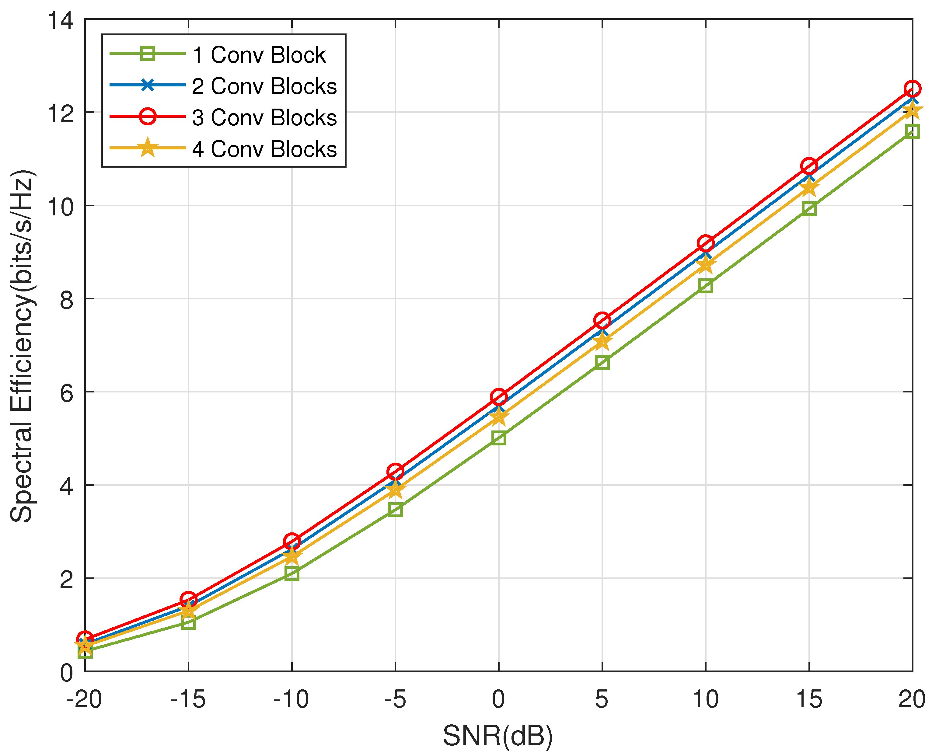
• We develop a DL-based approach for the joint optimization of digital and analog beamformers under the SE maximization problem. To solve the nonconvex problem, we propose a novel CNN-based HBF network framework with multiple convolutional blocks to efficiently extract more channel features. The proposed CNN structure can predict analog beamforming solution quickly and achieve excellent performance with low complexity, due to the parameter sharing feature of its convolutional operations. We also select the ELU activation function to speed up the convergence and employ dropout to avoid the risk of overfitting.
• We take an unsupervised deep-learning strategy to train the proposed CNN structure for the hybrid beamforming optimization problem. Unlike supervised CNNs, the devised unsupervised CNN updates the weights just based on the loss function without any optimal beamformer as labeled data, which is normally calculated by traditional algorithms. In addition, actually, there is no useful algorithm to find the global optimum due to the nonconvex nature of the problem. We only need to take CSI as input data for training to obtain feasible beamforming solutions adaptively. Thus, a huge amount of time and computational resources can be saved and the problem of data acquisition can be solved efficiently.
• To perform HBF optimization, we first train the neural network offline with a self-defined loss function and continuously learn to optimize the parameters, and then feed the saved model weight parameters into the trained network for online testing. This approach shifts the computational complexity from online testing to offline training, which can significantly lower the computational complexity of the online testing stage.
• Distinct from previous works, the performance of the proposed HBF algorithm with other algorithms in terms of the generalization ability for multiple CSIs is not only investigated, but we also innovatively discuss the performance of the mentioned algorithms with respect to the specific solving capability for a single CSI. We innovatively apply DL to the HBF optimization problem from this new perspective, which has not been mentioned in prior work. Simulation experiments are conducted in two classical channel environments, namely, a Rayleigh fading channel and geometric mmWave channel, respectively.

1.2. Paper Organization

The rest of the paper is organized as follows. Section 2 presents the system model and HBF optimization problem formulation in the downlink MISO system. Section 3 proposes the CNN-based architecture to optimize HBF, and introduces the training strategy of the network as well as analyzes the complexity of the mentioned algorithm. Simulation results are introduced in Section 4 and the conclusion is drawn in Section 5.

2. System Model and Problem Formulation

2.1. System Model

We consider a downlink MISO communication system, shown in Figure 1, which transmits data to the user by a HBF transmitter. In this scenario, a BS equipped with a single RF chain and $N_t$ antennas transmits a data stream to a single antenna user in an ideal channel environment. We assume that the BS at the transmitter is equipped with a uniform linear array (ULA) consisting of $N_t$ antenna units. Generally, the antenna spacing r is half of the transmission wavelength $\lambda$, i.e., $r=0.5\lambda$. The input signal s at BS obeys a complex Gaussian distribution with mean 0 and variance 1, i.e., it satisfies $s\sim \mathcal{C}\mathcal{N}(0,1)$.

In the HBF system, the input signal s first passes through the digital beamformer $v_{\mathrm{D}}$, which is actually a scalar since there is only one RF chain at the transmitter side. The signal s is then converted to analog phase shifters through one RF chain, and then the transmit signal $\mathbf{x}={\mathbf{v}}_{\mathrm{A}}{v}_{\mathrm{D}}s\in {\mathbb{C}}^{N_t\times 1}$ is constructed by passing through the analog beamforming vector ${\mathbf{v}}_{\mathrm{A}}\in {\mathbb{C}}^{N_t\times 1}$. The whole downlink HBF vector can be expressed as $\mathbf{v}={\mathbf{v}}_{\mathrm{A}}{v}_{\mathrm{D}}$, where $\mathbf{v}$ is an $N_t\times 1$-dimensional complex vector. The transmit signal $\mathbf{x}$ then passes through a channel $\mathbf{h}$ to obtain the received signal y at the receiver side. The received signal at the user side is given as

$$\begin{array}{c}\hfill y={\mathbf{h}}^H{\mathbf{v}}_{\mathrm{A}}{v}_{\mathrm{D}}s+n,\end{array}$$

(1)

where $\mathbf{h}\in {\mathbb{C}}^{N_t\times 1}$ denotes the downlink channel gain complex vector. n stands for the additive Gaussian white noise obeying a complex Gaussian distribution with zero mean and variance ${\sigma }^2$, i.e., n satisfies $n\sim \mathcal{C}\mathcal{N}(0,{\sigma }^2)$. In addition, ${\sigma }^2$ represents the noise power. The achievable rate of the HBF system is then calculated as

$$\begin{array}{c}\hfill R={log}_2(1+\frac{|{\mathbf{h}}^H{\mathbf{v}}_{\mathrm{A}}{v}_{\mathrm{D}}{|}^2}{{\sigma }^2}).\end{array}$$

(2)

2.2. Problem Formulation

We assume that the analog beamformer is implemented by simple phase shifters with adjustable phase and nonadjustable amplitude. Under this assumption, the elements of the analog beamforming vector ${\mathbf{v}}_{\mathrm{A}}$ are constrained by constant modulus, i.e., $|{\left[{\mathbf{v}}_{\mathrm{A}}\right]}_i{|}^2=1,\forall i=1,2,\dots ,N_t$. The goal is to maximize the SE of the MISO system subject to the constant modulus constraint and transmit power constraint, which is formulated as

$$\begin{array}{cc}\hfill \underset{\mathbf{v}}{max}& {log}_2(1+\frac{|{\mathbf{h}}^H{\mathbf{v}}_{\mathrm{A}}{v}_{\mathrm{D}}{|}^2}{{\sigma }^2})\hfill \end{array}$$

(3a)

$$\begin{array}{cc}\hfill s.t.& |{\mathbf{v}}_{\mathrm{A}}{v}_{\mathrm{D}}{|}^2\le P_{max},\hfill \end{array}$$

(3b)

$$\begin{array}{cc}\hfill & |{\left[{\mathbf{v}}_{\mathrm{A}}\right]}_i{|}^2=1,\forall i=1,2,\dots ,N_t.\hfill \end{array}$$

(3c)

Since $\parallel {\mathbf{v}}_{\mathrm{A}}{\parallel }_F^2=N_t$, the constraint term (3b) is equivalent to $|v_{\mathrm{D}}{|}^2\le P_{max}/N_t$. Moreover, the rate function is monotone increasing on $|v_{\mathrm{D}}{|}^2$, which means the equality of (3b) must be satisfied; otherwise, the rate can be further improved by increasing the transmit power. The optimal digital precoding parameter is then given by $v_{\mathrm{D}}^{*}=\sqrt{\frac{P_{max}}{N_t}}$. As a result, the HBF optimization problem (3) is degenerated to find the optimal analog beamforming vector, which is written as

$$\begin{array}{cc}\hfill \underset{{\mathbf{v}}_{\mathrm{A}}}{max}& {log}_2(1+\frac{P_{max}{\left|{\mathbf{h}}^H{\mathbf{v}}_{\mathrm{A}}\right|}^2}{N_t{\sigma }^2})\hfill \end{array}$$

(4a)

$$\begin{array}{cc}\hfill s.t.& |{\left[{\mathbf{v}}_{\mathrm{A}}\right]}_i{|}^2=1,\forall i=1,2,\dots ,N_t.\hfill \end{array}$$

(4b)

Problem (4) is still nonconvex due to the constant modulus constraint, and, thus, hard to solve. Recently, an FCNN-based deep-learning method is proposed to solve this, in [19]. Although the FCNN-based method is verified to be effective in finding a solution, it is not known whether a better solution can be achieved by other deep-learning methods. This motivates our work in this paper to develop a different neural network architecture on top of CNN to solve the analog beamforming optimization problem (4).

3. Proposed CNN-Based Hybrid Beamforming Optimization

In this section, we propose a CNN-based framework to solve the HBF optimization problem. CNN was chosen since it not only has better feature-extraction capability, but can also reduce the number of learning parameters by sharing weights and biases through convolution kernels, which has the potential to improve performance with low computational complexity. We also derive an unsupervised scheme to train the CNN.

3.1. Data Preparation

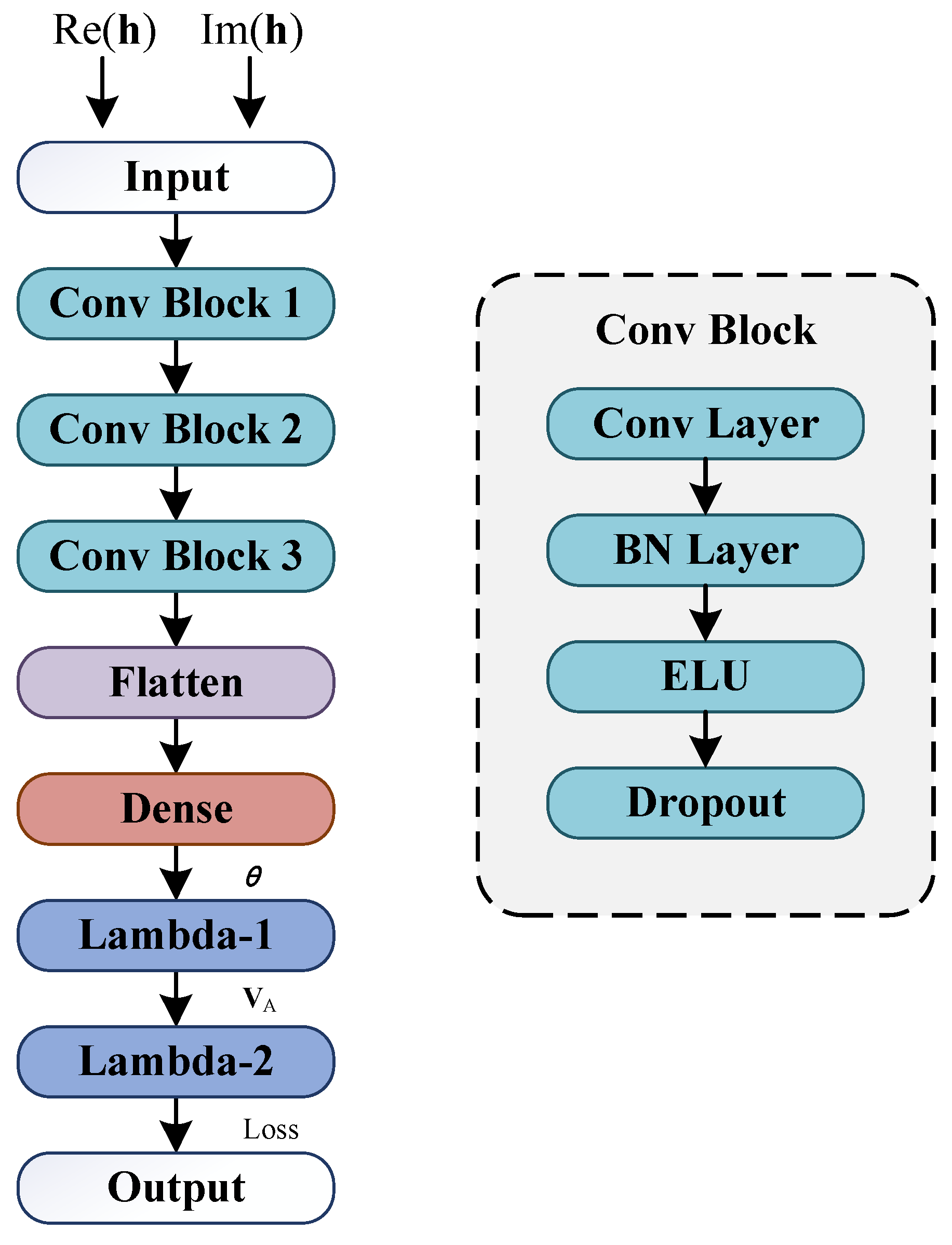
It is essential to perform data preprocessing on the input of the neural network, which aims to reduce the number of computations for subsequent training of the network. Following the CSI model of an HBF communication system, we perform data acquisition for channel $\mathbf{h}$. It will be extremely hard to train the network if a set of complex numbers as input is fed to the neural network directly to form a complex neural network. However, both the channel and beamforming vectors are essentially complex. Therefore, it is necessary to convert each input channel sample to real form. To simplify complex operations, we convert the complex CSI vector $\mathbf{h}$ into its corresponding real part and imaginary part, which is fed to the neural network. In this work, we split the real and imaginary part of each complex channel vector and rearrange them into a three-dimensional (3-D) real matrix with size 1 × $N_t$ × 2 in an element-wise manner. The samples are fed into the network in batches during the train stage.

3.2. CNN Structure

Our designed CNN structure is shown in Figure 2, which consists of an input layer, multiple convolutional (Conv) blocks, a fully connected layer, two self-defined layers, and an output layer. Each Conv block includes a Conv layer, a batch normalization (BN) layer, an activation layer and a dropout layer inside. The hyperparameter settings of each layer are shown in

Table 1. Parameters of the Proposed DL-based HBF Model.

Layer	${\mathit{N}}_{\mathit{o}}\times {\mathit{C}}_{\mathit{o}}$	Activation Function	Number of Parameters (When ${\mathit{N}}_{\mathit{t}}=64$)
Input	$N_t\times 2$	-	0
Conv Block 1	$\left(N_t-2\right)\times 16$	ELU	176
Conv Block 2	$\left(N_t-4\right)\times 8$	ELU	424
Conv Block 3	$\left(N_t-6\right)\times 4$	ELU	116
Flatten	$4\left(N_t-6\right)$	-	0
Dense	$N_t\times 1$	Sigmoid	14,912
Lambda-1	$N_t\times 1$	-	0

. A brief description of these network layers is given below.

3.2.1. Input Layer

The first layer is the input layer for receiving the input samples. It is a three-dimensional (3-D) matrix with real numbers of size $1\times N_t\times 2$ with two channels, as the input of the first Conv layer. Specifically, we split the real and imaginary part of each complex channel vector and rearrange them into a 3-D real matrix with size $1\times N_t\times 2$ in an element-wise manner.

3.2.2. Conv Blocks

We adopted three Conv blocks for feature extraction. Each Conv block is composed of a Conv layer, a BN layer, an activation layer and a dropout layer. The Conv layer takes the input signal and convolves it by convolution kernels to produce the output signal. Specifically, the Conv layer employs $C_o$ kernels of size $1\times 3$ with stride 1 to perform feature extraction for the real and imaginary parts of the input channel matrix, respectively. The BN layer normalizes the output of the Conv layer. BN is a regularization technique that prevents overfitting and achieves faster learning, thus accelerating convergence. The exponential linear units (ELU) activation function performs activation on the output of the BN layer. Considering that the beamformers may contain negative elements, we innovatively chose ELU as the nonlinear activation function of the proposed network model. This can alleviate the gradient disappearance problem by positive value identification, while having better robustness to negative value input. Further, it attempts to take the output average value of the activation function close to zero, thus speeding up the convergence rate. After that, we innovatively add the dropout layer, which is a technique that forces the output of some neurons to zero with random probability, and thus reduces the impact caused by the initial weight selection. This makes the network not overly dependent on some local features and thus improves the generalizability of the network. The random probability is set to 0.05 to avoid the over-regularization problem.

3.2.3. Flatten Layer

After extracting the features from the CNN blocks, the flatten layer converts these multi-dimensional features into a one-dimensional vector.

3.2.4. Dense Layer

The dense layer consists of $N_t$ neurons, which are connected to the outputs of the flatten layer. In order to improve convergence, we added a BN layer before the dense layer, which is omitted in Figure 2 for simplicity. The output of the dense layer corresponds to the phase vector $\mathit{\theta }$ of the analog beamformer, which can be used to construct the analog beamformer through the relationship of ${\mathbf{v}}_{\mathrm{A}}=e^{j2\pi \mathit{\theta }}$. The sigmoid activation function is used to map the output of the neurons of the dense layer to the range of (0, 1). The activated output vector of this layer is denoted as

$$\begin{array}{c}\hfill {\mathbf{c}}_o=\mathrm{Sig}\left(x\right)\left({\mathbf{W}}_o{\mathbf{c}}_i+{\mathbf{b}}_o\right),\end{array}$$

(5)

where $\mathrm{Sig}\left(x\right)\triangleq \frac{1}{1+e^{-x}}$ denotes the sigmoid activation function, ${\mathbf{c}}_o\in {\mathbb{R}}^{N_t\times 1}$, ${\mathbf{W}}_o\in {\mathbb{R}}^{N_t\times 4\left(N_t-6\right)}$, ${\mathbf{c}}_i\in {\mathbb{R}}^{4\left(N_t-6\right)\times 1}$ and ${\mathbf{b}}_o\in {\mathbb{R}}^{N_t\times 1}$ represent output vector, weight matrix, input vector and bias vector of this layer, respectively.

3.2.5. Lambda Layers

Since we expect to obtain the analog beamformer through the relationship ${\mathbf{v}}_{\mathrm{A}}=e^{j2\pi \mathit{\theta }}$, we devised a lambda layer for such a transform, which is named as Lambda-1 in Figure 2 and the output of which is ${\mathbf{v}}_{\mathrm{A}}$. Through the Lambda-1 layer, we map the real value of $\mathit{\theta }$ into complex values of ${\mathbf{v}}_{\mathrm{A}}$. Moreover, we further devised the Lambda-2 layer to convert the analog beamformer ${\mathbf{v}}_{\mathrm{A}}$ into a real value through a function $F_{\mathrm{Loss}}\left(v_{\mathrm{D}}^{*},{\mathbf{v}}_{\mathrm{A}}\right)\triangleq -R$, which denotes the loss function and is defined as the negative of the rate function. We note that the output layer is used also as the loss function; this is one key point to design an unsupervised training scheme, which will be described in the following.

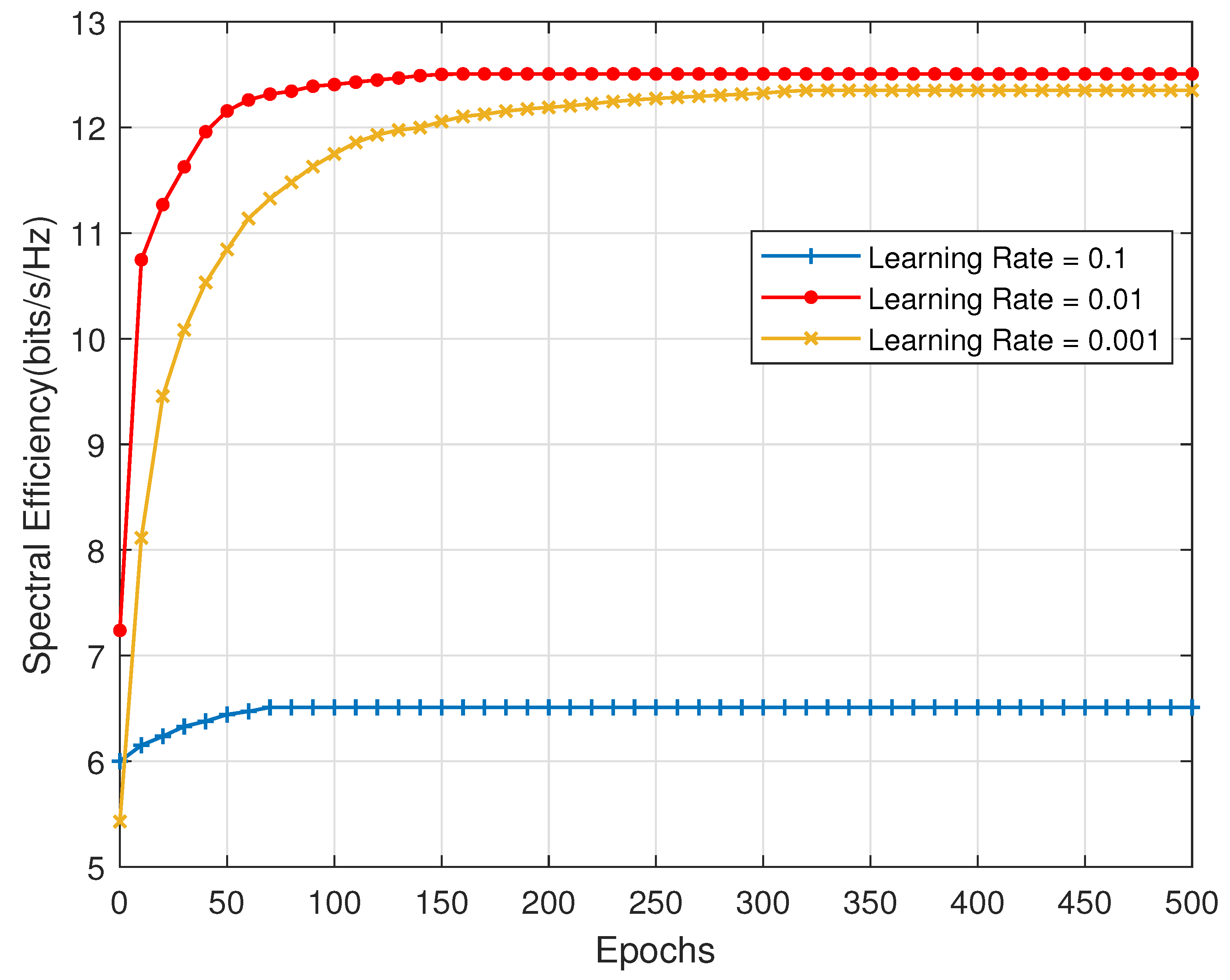
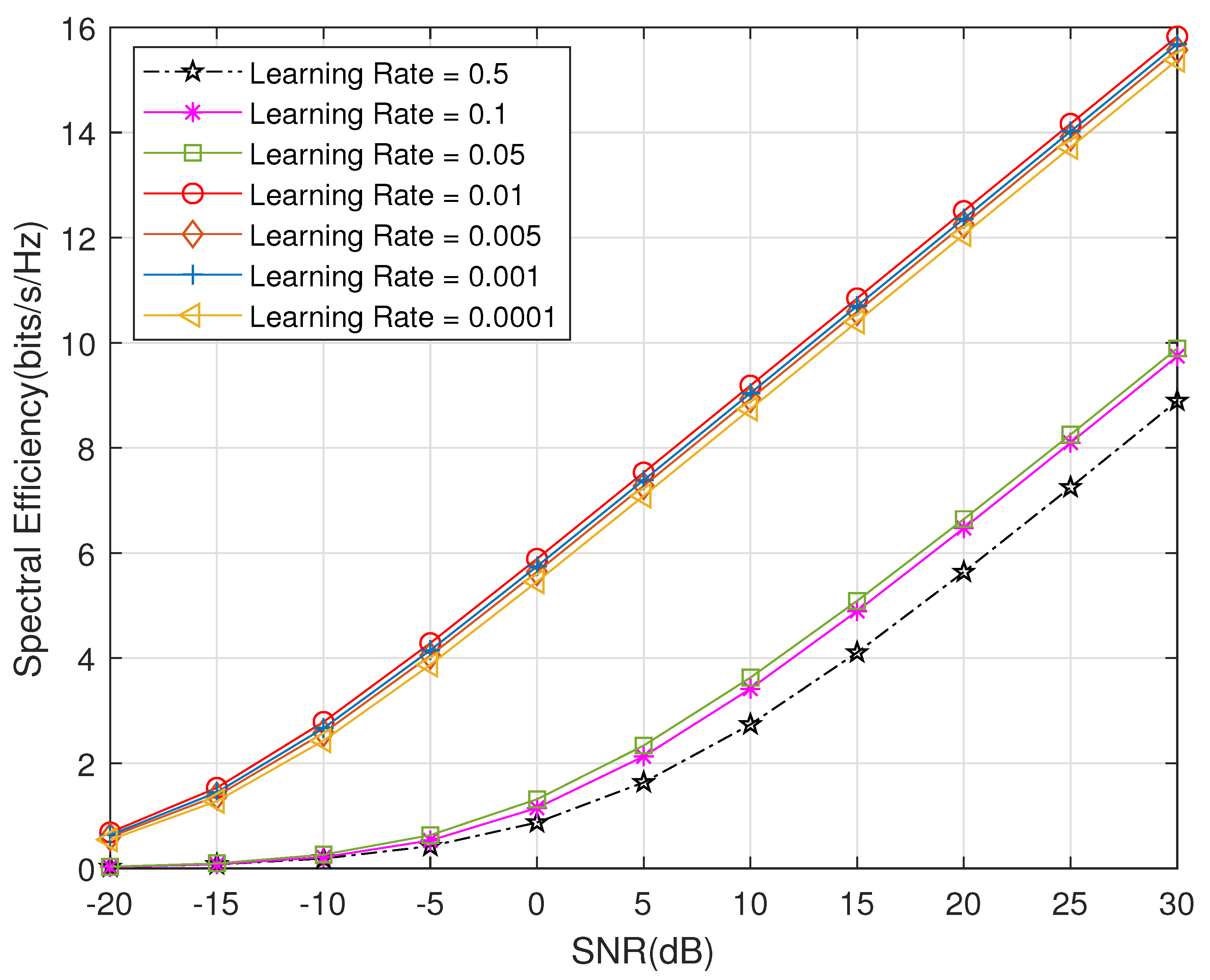
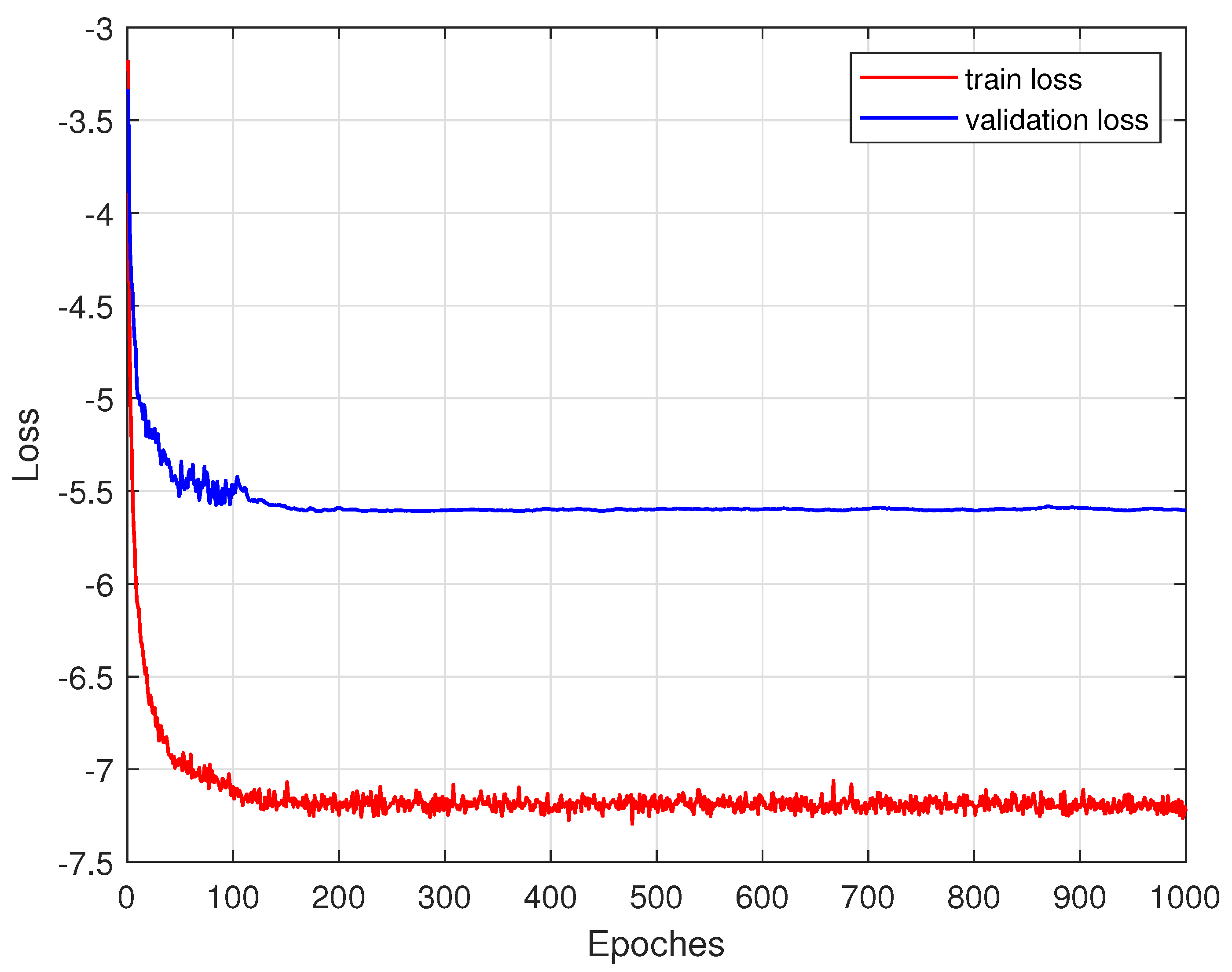
3.3. Training Strategy

The goal of the training is to find a feasible analog beamformer by maximizing the SE. The channel samples are fed into the proposed CNN-based model in batches for offline training. Note that the training weights are saved during the training process. The proposed CNN-based model is trained by 1000 epochs with 16 batches per epoch. The Adam optimizer is used to update the network parameters, such as weights and biases, with the initial learning rate of 0.01. A learning rate dynamic decay strategy is also used. Specifically, if no improvement in model performance was seen during 20 epochs, the learning rate was reduced by the factor of 0.2. Unlike other supervised CNNs, the proposed CNN model is trained using the unsupervised learning mechanism, which is achieved through the Lambda-2 layer. Recall that the Lambda-2 is designed to be the loss function, the output of which is the negative of the rate. By defining such a Lambda function, we can train CNN without using the labeled data, i.e., the optimal analog beamformers for the given CSI samples, and, thus, achieve unsupervised learning for the constructed network. The parameters of the CNN network are then optimized though batch optimization. For a given training batch, the parameters are updated by minimizing the loss

$$\begin{array}{c}\hfill F_{\mathrm{Loss}}=-\frac{1}{N}\sum _{n=1}^N{log}_2(1+\frac{{\gamma }_n{\left|{\mathbf{h}}_n^H{\mathbf{v}}_{\mathrm{A}}^{\left(n\right)}\right|}^2}{N_t})\end{array}$$

(6)

where N denotes the total number of training samples in a batch. ${\gamma }_n=\frac{P_{max}}{{\sigma }^2}$, ${\mathbf{h}}_n$ and ${\mathbf{v}}_{\mathrm{A}}^{\left(n\right)}$ represent the SNR value, channel vector, and analog beamforming vector of the n-th sample in the training batch.

3.4. Complexity Analysis

Considering only the online stage, we compared the complexity of the proposed CNN-based HBF scheme, the FCNN-based scheme [19] and the traditional HBF schemes [12,13] in terms of the number of parameters and FLOPs. Assume that the number of input neurons in each layer is $N_i$, the number of output neurons is $N_o$, the number of input channels is $C_i$, and the number of output channels is $C_o$. Each Conv layer consists of $C_o$ kernels of size $1\times z$, where we set $z=3$, and we also learn that $N_o=N_i-z+1$ for each Conv layer. When calculating FLOPs, the bias is considered, so the number of FLOPs in the Conv layer is $2\times z\times C_i\times C_o\times N_o$, and the number of FLOPs in the dense layer is $2\times N_i\times N_o$. According to the parameters shown in Table 1, it can be calculated that the total number of FLOPs for the proposed CNN-based algorithm is about 0.09 million, the number of FLOPs for the FCNN-based algorithm [19] is around 0.15 million while $N_t=64$. However, the traditional HBF schemes, such as [12,13], have higher complexity due to a large number of complex iterative operations, and the number of FLOPs is approximately 0.26 million. The detailed complexity comparison when $N_t=64$ is shown in

Table 2. Complexity comparison.

HBF Scheme	Number of Parameters	Number of FLOPs
Proposed CNN-based	16,556	0.09 million
FCNN-based [19]	75,720	0.15 million
Traditional	-	0.26 million

. The analysis of the number of parameters and FLOPs shows the great superiority of the proposed CNN-based scheme over other schemes in terms of complexity. Moreover, the significant reduction in complexity leads to an increase in execution speed. We also compared the average execution time of the proposed CNN-based HBF scheme, the FCNN-based scheme, as well as the two traditional schemes, as shown in

Table 3. Execution time comparison.

HBF Scheme	Execution Time
Proposed CNN-based	0.3223 s
FCNN-based [19]	0.3338 s
Traditional [12]	11.9553 s
Traditional [13]	9.5333 s

, where we set $N_t=64$. It can be noticed that the traditional scheme [12] has the highest execution time, followed by scheme [13]. The execution times of the two traditional HBF schemes are much higher than the two schemes using DL. In particular, the proposed CNN-based algorithm has a shorter average execution time compared to FCNN. Overall, it is observed that the proposed algorithm has a superior advantage over other algorithms both in terms of complexity and execution time.

4. Simulation Results

We consider a downlink MISO system model where a BS equipped with $N_t$ transmit antennas and one RF chain serves a single-antenna user for HBF design. In the simulation section, we discuss the performance of the proposed algorithm in terms of both the generalization ability for multiple CSIs and the specific solving ability for an individual CSI, respectively. This section verifies the performance of the proposed unsupervised CNN-based HBF algorithm using simulation experiments. To compare the performance, several solving schemes based on traditional optimization techniques and FCNN are employed in the experiments, including:

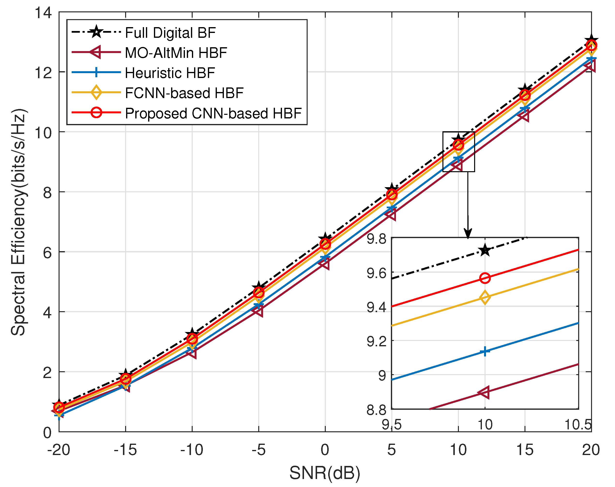
• Full digital beamforming algorithm: This algorithm (labeled with ’Full Digital BF’) is a digital beamforming technique based on singular value decomposition (SVD). Although the optimal performance can be achieved theoretically, it will face the issues of high overhead, high implementation complexity and high power consumption in large-scale antenna arrays.
• Traditional HBF algorithm [12]: This scheme (labeled with ’MO-AltMin HBF’) approximates the HBF optimization problem as a matrix factorization problem with alternate optimization of analog and digital beamforming. However, it imposes a performance loss and fails to obtain optimal results.
• Traditional HBF algorithm [13]: This method (labeled with ’Heuristic HBF’) is an element-based heuristic HBF iterative algorithm that optimizes the beamforming matrix while taking the performance metric as the optimization objective directly. Yet, it requires numerous iterative operations with high computational complexity and long execution time.
• FCNN-based HBF algorithm [19]: This scheme employs DL network architecture to optimize HBF, but its use of multiple fully connected layers suffers from the issue of excessive weight parameters, which may raise the computational complexity.

The simulation experiment environment is deployed on a computer with Windows 10 OS as well as NVIDIA GeForce GTX 1650 GPU and Intel(R) Core(TM) i7-10750 CPU, and the model training is based on Python 3.7 and Tensorflow 2.0.0.

4.1. Channel Model

The proposed optimization algorithm can efficiently achieve feasible beamforming solutions once the channel parameters are given. It is especially noted that the algorithm can be applied for any channel environments. Specifically, we use two typical channel models (i.e., Rayleigh fading channel and geometric mmWave channel) as the channel $\mathbf{h}$ between BS and user for correlation simulations. We summarized the model generating methods and properties for the Rayleigh fading channel and geometric mmWave channel in

Table 4. Channel Models for Algorithm Evaluation.

-	Rayleigh Fading Channel	Geometric mmWave Channel
Model generation	$h_i\sim \mathcal{C}\mathcal{N}(0,1)$	${\mathbf{h}}^H=\sqrt{\frac{N_t}{L}}{\sum }_{l=1}^L{\alpha }_l{\mathbf{a}}_t^H\left({\theta }_l\right)$
Properties	✓ Non LoS path; ✓ Rich scattering environment surrounding the receiver.	✓ One LoS path; ✓ Directional transmission due to short wavelength or no scattering objectives near the receiver.

.

Among them, the Rayleigh fading channel assumes that the signal amplitude is random after it passes through the wireless channel. Suppose $h_i$ denotes the i-th element of the vector $\mathbf{h}$. Each element of this channel is an independent and identically distributed (i.i.d.) zero-mean circularly symmetric complex Gaussian random variable, i.e., $h_i\sim \mathcal{C}\mathcal{N}(0,1)$.

Beyond the ideal Rayleigh fading channel, our proposed HBF optimization algorithm can be employed for mmWave communication with very limited clusters, which suffers from severe free-space path loss during propagation. Consequently, a geometric mmWave channel model with the same parameters as presented in [23] is considered, which can be expressed as

$${\mathbf{h}}^H=\sqrt{\frac{N_t}{L}}\sum _{l=1}^L{\alpha }_l{\mathbf{a}}_t^H\left({\theta }_l\right),$$

(7)

where $L=3$ denotes the number of clusters between the BS and the user and each scattering cluster contributes a single propagation path, where one line-of-sight (LoS) path is adopted. Meanwhile, ${\alpha }_l\sim \mathcal{C}\mathcal{N}(0,1)$ stands for the complex gain of the l-th cluster. ${\mathbf{a}}_t\left({\theta }_l\right)=\frac{1}{\sqrt{N_t}}{[1,e^{j\frac{2\pi r}{\lambda }sin\left({\theta }_l\right)},\dots ,e^{j\frac{2\pi r}{\lambda }\left(N_t-1\right)sin\left({\theta }_l\right)}]}^T$ indicates the transmitting antenna array response vector at the BS, and, furthermore, ${\theta }_l$ is the azimuth angles of departure (AoD) of the l-th cluster drawn independently from uniform distributions over $[0,2\pi ]$.

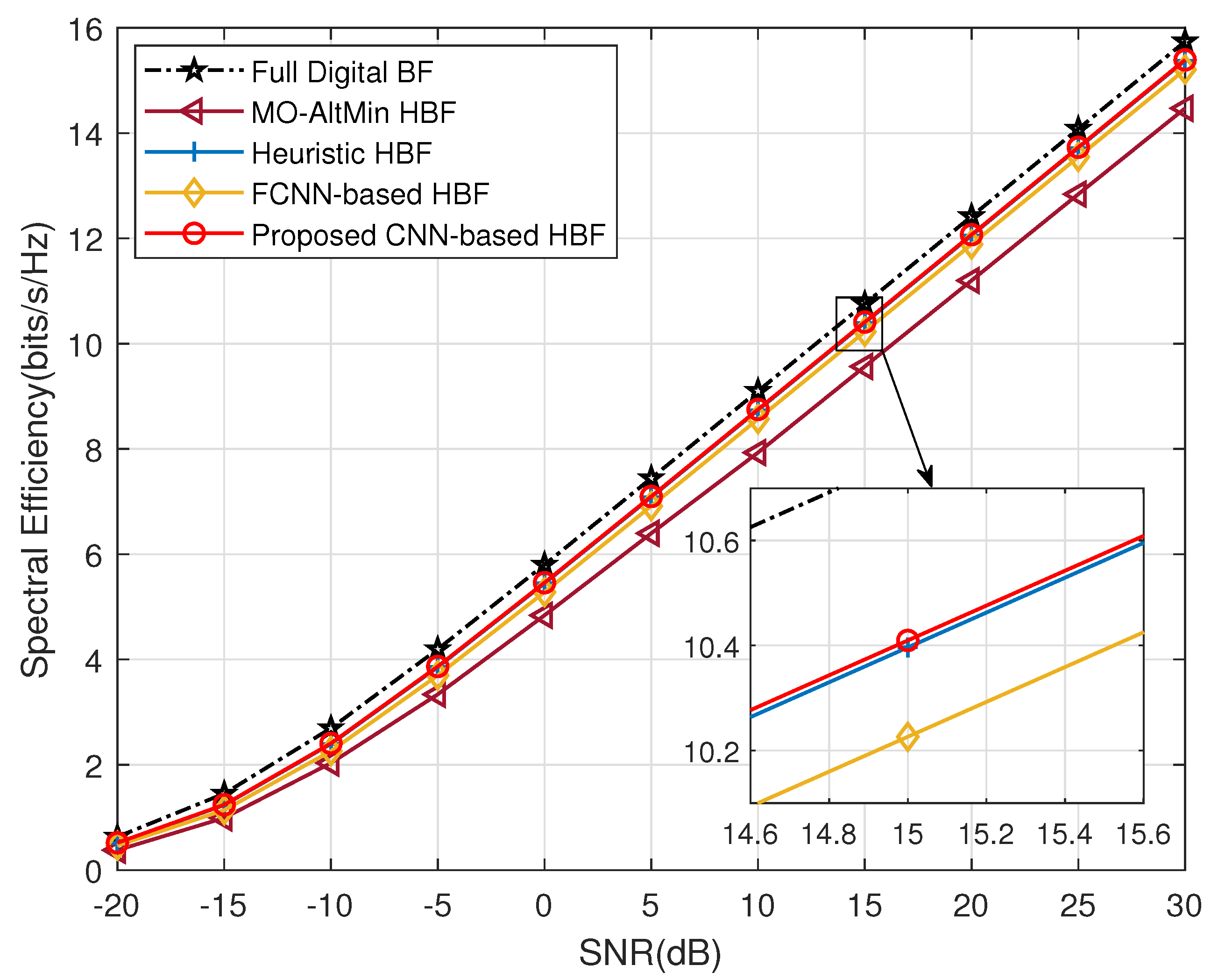
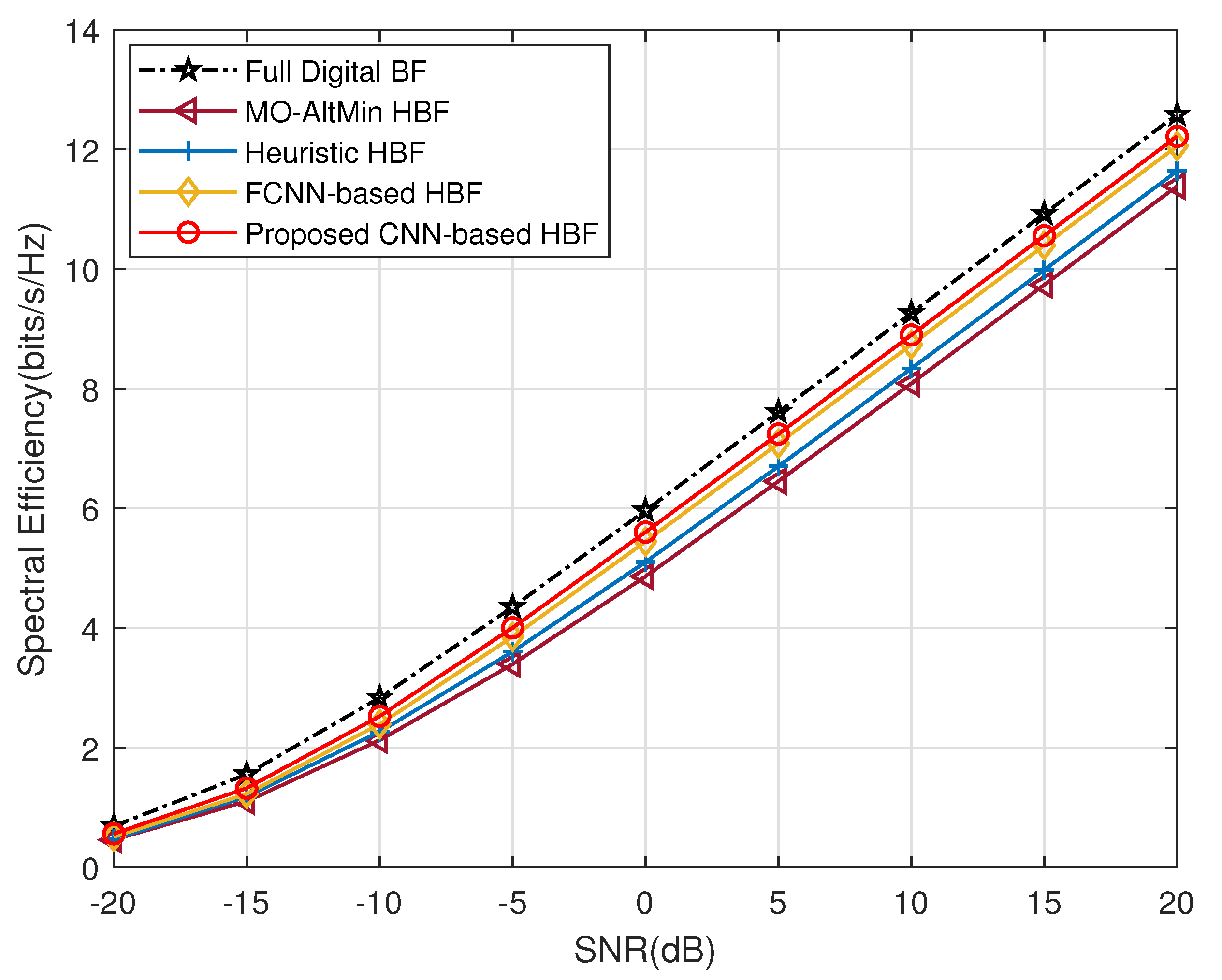
4.2. Generalization for Multiple CSIs

To ensure the generality of the network, we gave different realizations of $\mathbf{h}$ to construct two datasets, each consisting of 100 channel samples. A total of $90\%$ of the first dataset was selected as the set for training the network model, and the remaining $10\%$ was used as the validation set. The validation set was used to adjust the hyperparameters of the neural network model during the training process to maximize the generalization ability of the model to achieve the accurate prediction of new data, where the generalization ability refers to the ability of the model to adapt to new samples. The second dataset was used as the test set to evaluate the final performance of the model. All simulation results were obtained by taking the average of all channel realizations.

Figure 3 shows the SE performance when the number of Conv blocks is 1, 2, 3, and 4 respectively. To facilitate the comparison, the networks in the four cases are set such that the number of parameters to be trained are the same, which makes sure that the computational complexity of the four cases are the same. We explore the effect of various numbers of Conv blocks on the SE and complexity of the proposed network model. It can be seen that the network with three Conv blocks has the best performance, while one Conv block has the worst one. For the cases of one Conv block and two Conv blocks, the generalization ability is limited. Although it is possible to use more filters to achieve a similar performance as that of three Conv blocks, it will cause very high complexity since the width of the neural networks should be drastically increased. The four Conv blocks exhibit lower SE compared to the three Conv blocks with the same complexity and fail to attain the desired performance. The reason for this is that the deepening of the network causes the gradient to be unstable and the performance will be degraded instead. We use three Conv blocks for subsequent experiments, since networks with three Conv blocks can achieve better SE performance with low complexity.

The learning rate setting is crucial when training the model, because it controls the magnitude of parameters updated per time. Figure 4 shows the convergence of the proposed scheme under various learning rates with $N_t=64$, SNR = 20 dB. It is observed that the learning rate of 0.1 converges to stability in about 70 epochs with the fastest convergence rate, but it has the lowest SE value. The learning rate of 0.01 tends to stabilize in about 170 epochs and has the highest SE value. In addition, the learning rate of 0.001 becomes stable in about 330 iterations. Figure 5 compares the SE performance versus SNR of the proposed scheme under various learning rates in large geometric mmWave channel with $N_t=64$. Obviously, the learning rate setting of 0.01 has the highest SE value, while setting it to 0.5 or 0.0001 will not give excellent SE performance. This is because too high a learning rate will cause larger update amplitude and the parameters to be optimized fluctuate around the minimum value and do not converge, while too low will cause slow convergance.

Figure 6 illustrates the convergence performance of the proposed CNN structure with 1000 epochs and a learning rate of 0.01 in large geometric mmWave channel with $N_t=64$. At the beginning of the training stage, the training weight parameters are not optimal. Thus, the loss values for the first few epochs are quite large. As the training proceeds, the parameters tend to be optimal and the loss decreases abruptly. After that, the system loss function tends to be stable with very small fluctuations and low loss values.

Figure 7 gives the comparison of SE performance under different beamforming schemes in large Rayleigh fading channel with $N_t=64$. The full digital beamforming method provides higher SE compared to HBF schemes. It can be seen that, under the same channel samples, the proposed CNN-based HBF scheme achieved better performance than traditional HBF iterative algorithms, and obtained higher SE than the FCNN-based scheme. Moreover, we performed the simulation experiments under different antenna configurations to reflect the generality of the model. Specifically, Figure 8 shows the SE achieved by different beamforming schemes in large Rayleigh fading channel with $N_t=128$. All schemes show a significant improvement in SE values due to the increased number of antennas. It can also be clearly seen that the proposed CNN has much higher SE than other HBF algorithms.

Furthermore, except for Rayleigh fading channels, our proposed HBF design scheme is also applicable to large mmWave channel with limited clusters. Figure 9 compares the performance of the proposed algorithm with other beamforming algorithms in large geometric mmWave channel when $N_t=64$. The performance of our proposed algorithm is improved upon only by the fully digital beamforming algorithm. In addition, our proposed CNN-based scheme still has a higher SE performance compared to the traditional HBF algorithms and FCNN. Similarly, we present the achieved SE of various beamforming algorithms in large geometric mmWave channel under different antenna configurations, as shown in Figure 10. It is equally noticed that the SE performance of the proposed CNN solution is close to that of the optimal fully digital beamforming solution, and significantly outperforms the traditional heuristic HBF algorithm [13] and FCNN.

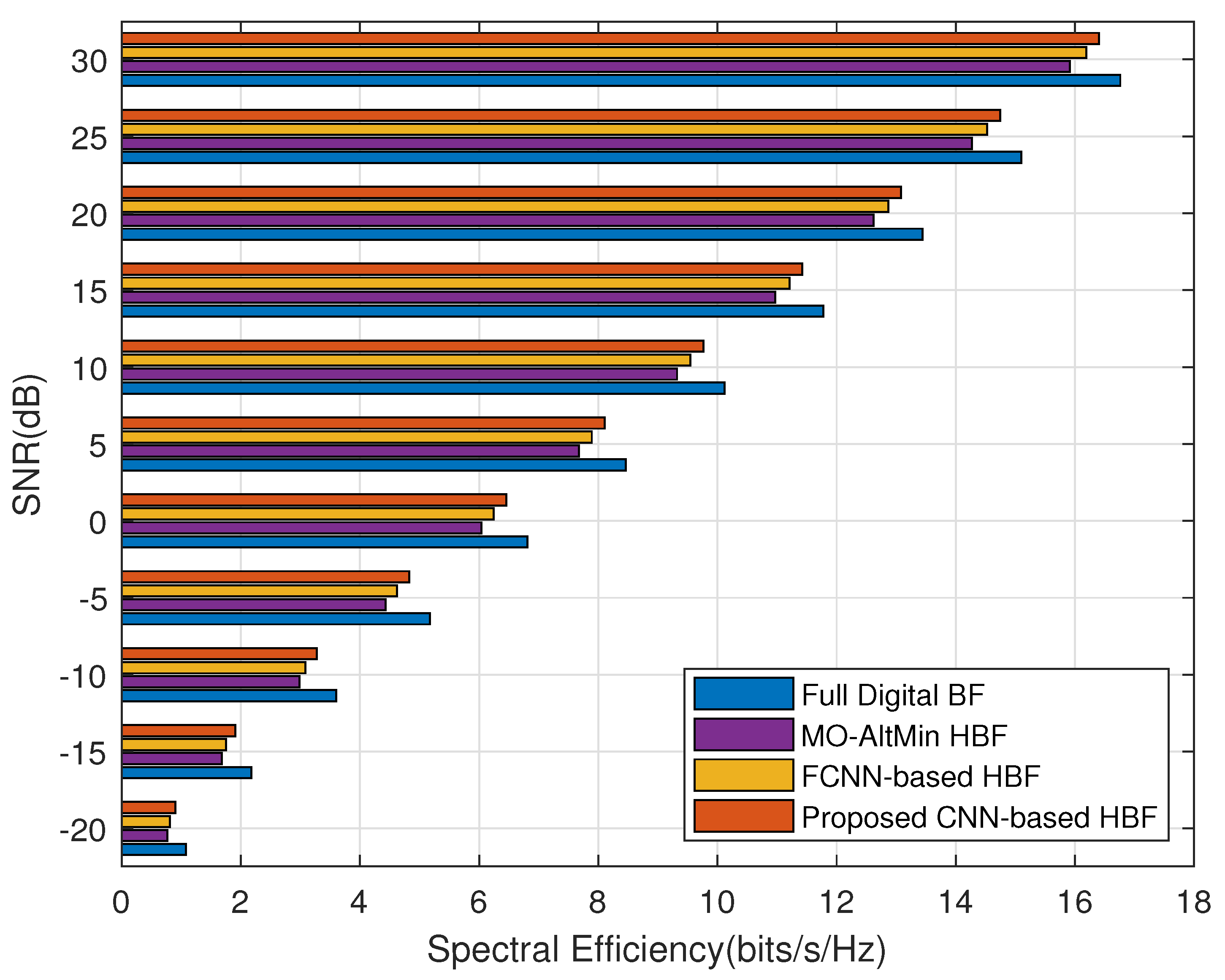
4.3. Specific Solution for an Individual CSI

The comparison of the generalization ability of the proposed HBF method against other algorithms for multiple CSIs is discussed above. Existing DL-based studies mostly discuss the above aspect, specifically feeding numerous different channel implementations into the framework and then computing the average SE performance of these multiple CSIs. However, they lack the specific solution for any individual CSI. Different from previous works, we also innovatively discuss the specific solving capability of the mentioned HBF algorithm for an individual CSI in this work. For this part, as long as a CSI is given, we can feed it into the proposed neural network framework for training to efficiently calculate the feasible specific solution for this CSI, which is applicable to all channel conditions. The following simulation experiments are conducted in terms of the specific solution for an individual CSI under both Rayleigh fading channel and geometric mmWave channel, respectively.

Figure 11 shows the SE performance of our proposed HBF algorithm compared to other algorithms in large Rayleigh fading channel with $N_t=64$. As shown in Figure 11, we can clearly see that, similar to the part of the generalization of multiple CSIs, the proposed algorithm still has better SE performance compared to the traditional HBF algorithms and FCNN in terms of the specific solving for a single CSI. Furthermore, Figure 12 plots the SE versus SNR for different HBF schemes in large geometric mmWave channel with $N_t=64$. With increasing SNR, the proposed CNN-based scheme outperforms the traditional HBF algorithms and FCNN-based scheme. Our proposed algorithm has a performance similar to that of the optimal solution for full digital beamforming.

As mentioned above, the proposed algorithm performs better than the traditional HBF algorithms as well as the FCNN-based algorithm in both the generalization capability for multiple CSIs and the specific solving capability for an individual CSI. Since FCNN has the ability to adopt a global perceptive, FCNN has a serious issue, i.e., there are too many parameters. While CNN can achieve local perception, the weights of different neurons in the Conv layer are shared, which greatly reduces the parameters and improves the training performance of the whole network, and can extract features more effectively. Meanwhile, CNN can handle the coupling between different elements more efficiently than FCNN [21]. It is shown that the proposed CNN model obtained superior performance compared to FCNN.

5. Conclusions

In this work, we presented a low-complexity HBF optimization algorithm for a downlink MISO system with a CNN-based network architecture and an unsupervised learning mechanism for training. We compared the performance of the mentioned algorithms in terms of the ability of both generalization of multiple CSIs and specific solving of an individual CSI, respectively. Simulation results confirmed the feasibility of the proposed scheme. A comparison of the proposed scheme with other existing works was presented with respect to complexity and SE performance. Compared with traditional HBF algorithms and FCNN, the CNN-based HBF algorithm we proposed obtains superior SE performance with lower complexity. The work that we performed offers a novel approach to the HBF design and delivers an innovative new idea for the optimization problem.

References

1. Andrews, J.G.; Buzzi, S.; Choi, W.; Hanly, S.V.; Lozano, A.; Soong, A.C.; Zhang, J.C. What will 5G be? IEEE J. Sel. Areas Commun. 2014, 32, 1065–1082. [Google Scholar] [CrossRef]
2. Niu, Y.; Li, Y.; Jin, D.; Su, L.; Vasilakos, A.V. A survey of millimeter wave communications (mmWave) for 5G: Opportunities and challenges. Wirel. Netw. 2015, 21, 2657–2676. [Google Scholar] [CrossRef]
3. Hong, S.H.; Park, J.; Kim, S.J.; Choi, J. Hybrid beamforming for intelligent reflecting surface aided millimeter wave MIMO systems. IEEE Trans. Wirel. Commun. 2022. [Google Scholar] [CrossRef]
4. Wiesel, A.; Eldar, Y.C.; Shamai, S. Zero-forcing precoding and generalized inverses. IEEE Trans. Signal Process. 2008, 56, 4409–4418. [Google Scholar] [CrossRef] [Green Version]
5. Cui, W.; Dong, A.; Cao, Y.; Zhang, C.; Yu, J.; Li, S. Deep learning based MIMO transmission with precoding and radio transformer networks. Procedia Comput. Sci. 2021, 187, 396–401. [Google Scholar] [CrossRef]
6. Zhang, T.; Yu, J.; Dong, A.; Qiu, J. Deep learning-based transceiver design for multi-user MIMO systems. Internet Things 2022, 19, 100512. [Google Scholar] [CrossRef]
7. Molisch, A.F.; Ratnam, V.V.; Han, S.; Li, Z.; Nguyen, S.L.H.; Li, L.; Haneda, K. Hybrid beamforming for massive MIMO: A survey. IEEE Commun. Mag. 2017, 55, 134–141. [Google Scholar] [CrossRef] [Green Version]
8. Zhang, X.; Molisch, A.F.; Kung, S.Y. Variable-phase-shift-based RF-baseband codesign for MIMO antenna selection. IEEE Trans. Signal Process. 2005, 53, 4091–4103. [Google Scholar] [CrossRef]
9. Mo, J.; Alkhateeb, A.; Abu-Surra, S.; Heath, R.W. Hybrid architectures with few-bit ADC receivers: Achievable rates and energy-rate tradeoffs. IEEE Trans. Wirel. Commun. 2017, 16, 2274–2287. [Google Scholar] [CrossRef]
10. El Ayach, O.; Rajagopal, S.; Abu-Surra, S.; Pi, Z.; Heath, R.W. Spatially sparse precoding in millimeter wave MIMO systems. IEEE Trans. Wirel. Commun. 2014, 13, 1499–1513. [Google Scholar] [CrossRef] [Green Version]
11. Hung, W.L.; Chen, C.H.; Liao, C.C.; Tsai, C.R.; Wu, A.Y.A. Low-complexity hybrid precoding algorithm based on orthogonal beamforming codebook. In Proceedings of the 2015 IEEE Workshop on Signal Processing Systems (SiPS), Hangzhou, China, 14–16 October 2015; pp. 1–5. [Google Scholar]
12. Yu, X.; Shen, J.C.; Zhang, J.; Letaief, K.B. Alternating minimization algorithms for hybrid precoding in millimeter wave MIMO systems. IEEE J. Sel. Top. Signal Process. 2016, 10, 485–500. [Google Scholar] [CrossRef] [Green Version]
13. Sohrabi, F.; Yu, W. Hybrid digital and analog beamforming design for large-scale antenna arrays. IEEE J. Sel. Top. Signal Process. 2016, 10, 501–513. [Google Scholar] [CrossRef] [Green Version]
14. Ren, Y.; Wang, Y.; Qi, C.; Liu, Y. Multiple-beam selection with limited feedback for hybrid beamforming in massive MIMO systems. IEEE Access 2017, 5, 13327–13335. [Google Scholar] [CrossRef]
15. Alkhateeb, A.; Alex, S.; Varkey, P.; Li, Y.; Qu, Q.; Tujkovic, D. Deep learning coordinated beamforming for highly-mobile millimeter wave systems. IEEE Access 2018, 6, 37328–37348. [Google Scholar] [CrossRef]
16. Huang, H.; Song, Y.; Yang, J.; Gui, G.; Adachi, F. Deep-learning-based millimeter-wave massive MIMO for hybrid precoding. IEEE Trans. Veh. Technol. 2019, 68, 3027–3032. [Google Scholar] [CrossRef] [Green Version]
17. Li, X.; Alkhateeb, A. Deep learning for direct hybrid precoding in millimeter wave massive MIMO systems. In Proceedings of the 2019 53rd Asilomar Conference on Signals, Systems, and Computers, Pacific Grove, CA, USA, 3–6 November 2019; pp. 800–805. [Google Scholar]
18. Xia, W.; Zheng, G.; Zhu, Y.; Zhang, J.; Wang, J.; Petropulu, A.P. A deep learning framework for optimization of MISO downlink beamforming. IEEE Trans. Commun. 2020, 68, 1866–1880. [Google Scholar] [CrossRef]
19. Lin, T.; Zhu, Y. Beamforming design for large-scale antenna arrays using deep learning. IEEE Wirel. Commun. Lett. 2020, 9, 103–107. [Google Scholar] [CrossRef] [Green Version]
20. Attiah, K.M.; Sohrabi, F.; Yu, W. Deep learning approach to channel sensing and hybrid precoding for TDD massive MIMO systems. In Proceedings of the 2020 IEEE Globecom Workshops (GC Wkshps), Taipei, Taiwan, 7–11 December 2020; pp. 1–6. [Google Scholar]
21. Song, H.; Zhang, M.; Gao, J.; Zhong, C. Unsupervised learning-based joint active and passive beamforming design for reconfigurable intelligent surfaces aided wireless networks. IEEE Commun. Lett. 2021, 25, 892–896. [Google Scholar] [CrossRef]
22. Kuo, C.H.; Chang, H.Y.; Chang, R.Y.; Chung, W.H. Unsupervised Learning Based Hybrid Beamforming with Low-Resolution Phase Shifters for MU-MIMO Systems. arXiv 2022, arXiv:2202.01946. [Google Scholar]
23. Alkhateeb, A.; El Ayach, O.; Leus, G.; Heath, R.W. Channel estimation and hybrid precoding for millimeter wave cellular systems. IEEE J. Sel. Top. Signal Process. 2014, 8, 831–846. [Google Scholar] [CrossRef] [Green Version]
Figure 1. SU-MISO system architecture with hybrid (analog and baseband) beamforming.
Electronics 11 02213 g001
Figure 2. The proposed neural network architecture for hybrid beamforming design.
Electronics 11 02213 g002
Figure 3. Spectral efficiency comparisons of the proposed scheme under various numbers of Conv blocks in geometric mmWave channel with N t = 64 .
Electronics 11 02213 g003
Figure 4. Spectral efficiency performance versus epochs of the proposed scheme under various learning rates in geometric mmWave channel with N t = 64 , SNR = 20 dB.
Electronics 11 02213 g004
Figure 5. Spectral efficiency performance versus SNR of the proposed scheme under various learning rates in geometric mmWave channel with N t = 64 .
Electronics 11 02213 g005
Figure 6. Convergence performance of the proposed scheme in geometric mmWave channel with N t = 64 .
Electronics 11 02213 g006
Figure 7. Comparison of spectral efficiency performance under different schemes in Rayleigh fading channel with N t = 64 .
Electronics 11 02213 g007
Figure 8. Comparison of spectral efficiency performance under different schemes in Rayleigh fading channel with N t = 128 .
Electronics 11 02213 g008
Figure 9. Comparison of spectral efficiency performance under different schemes in geometric mmWave channel with N t = 64 .
Electronics 11 02213 g009
Figure 10. Comparison of spectral efficiency performance under different schemes in geometric mmWave channel with N t = 128 .
Electronics 11 02213 g010
Figure 11. Comparison of spectral efficiency performance among different schemes about specific solution for an individual CSI in Rayleigh fading channel with N t = 64 .
Electronics 11 02213 g011
Figure 12. Comparison of spectral efficiency performance of different schemes about specific solution for an individual CSI in geometric mmWave channel with N t = 64 .
Electronics 11 02213 g012