Google Mobility Data as a Predictor for Tourism in Romania during the COVID-19 Pandemic—A Structural Equation Modeling Approach for Big Data

Abstract

Our exploratory research focuses on the possible relations between tourism and the mobility of people, using short longitudinal data for mobility dimensions during the COVID-19 pandemic. One of these is real-time, exhaustive type data, published by Google, about the mobility of people in six different dimensions, (retail, parks, residential, workplace, grocery, and transit). The aim is to analyze the directional, intensity, causal, and complex interplay between the statistical data of tourism and mobility data for Romanian counties. The main objective is to determine if real-world big data can be linked with tourism arrivals in the first 14 months of the pandemic. We have found, using correlations, factorial analysis (PCA), regression models, and SEM, that there are strong and/or medium relationships between retail and parks and overnights, and weak or no relations between other mobility dimensions (workplace, transit). By applying factorial analysis (PCA), we have regrouped the six Google Mobility dimensions into two new factors that are good predictors for Romanian tourism at the county location. These findings can help provide a better understanding of the relationship between the real movement of people in different urban areas and the tourism phenomenon: the GM parks dimension best predicts tourism indicators (overnights), the GM residential dimension correlates inversely with the tourism indicator, and the rest of the GM indices are generally weak predictors for tourism. A more complex analysis could signal the potential and the character of tourism in different destinations, by territorially and chronologically determining the GM indices that are better linked with the tourism statistical indicators. Further research is required to establish forecasting models using Google Mobility data.

1. Introduction

Tourism in Romania is a dynamic and well-developed service sector, with mountain [1] and seaside (the Black Sea Coast) destinations, ski resorts [2], health resorts with mineral and saltwater treatments, the Danube Delta, and cultural heritage sites, specifically located in the Moldova and Transylvania regions [3].

The number of overnights were around 44 million/year in 1990; this dropped to 16 million in 2010, but had recovered up to 30 million overnights in 2019 [4]. A total of 82% of these overnights were produced by domestic tourists, and most of the 5.3 million foreign tourist overnights (around 4 million) were spent in the capital of Bucharest and in other cities and county seats [4].

In 2020, the COVID-19 pandemic brought devastating setbacks for Romanian tourism: while globally, tourism arrivals decreased by 73% (to 37% of the previous year), in 2020 compared to 2019, according to the UNWTO [5] data dashboard, in Romania, this downturn was even more dramatic: tourist arrivals decreased by 83% in 2020 compared to 2019, according to the same source. The national statistics show that overnights in Romania decreased to 48% in 2020, compared to the previous year, but foreign visitors’ overnights dropped even more, to a level of 19% of those recorded for the year 2019 (thus, in 2020, only 6.8% of the total overnights came from foreign visitors) [4]. The impact of COVID-19 on human mobility varied significantly by country and place [6].

The research on tourism in Romania is based, to a large extent, on traditional statistical data (often not so accurate, due to reporting deficiencies) or on questionnaire-based primary research. In some research articles recently published about tourism in Romania, counting only the first ten search results from Google Scholar, for relevant articles published after 2018, six were based on questionnaires with tourists [7,8,9,10,11,12,13], three were based on case studies [14,15,16], and one was based on statistical data analyzed using GIS methods [17]. There were no articles found using big data or other data obtained from new technologies, such as mobile phone tracking data, application downloads, debit card records, social media data, or other location/mobility data providers) for Romania.

In the meantime, there is an explosion of research on tourism, the mobility of people in urban areas or between cities, using different kinds of big data. We found the following topics related to tourism and observational data:

• Flickr photo geotagging, to estimate visitor trajectories [18] or to analyze tourist behavior and expectations against destinations [19], Twitter geotagging, and Foursquare geotagging data in Japan, used to characterize locations based on the points of interest in a neighborhood [20];
• A variety of articles based on mobile phone data, from tourist group behavior observations with call detail records (CDR) analysis [21], to passive mobile data used to study the effects of tourism seasonality in local mobility patterns [22], to methods to discover and cluster hotspots regarding downloaded applications by tourists [23], to innovative mobile phone apps with integrated surveys and Global Navigation Satellite System (GNSS) technology to examine the movements of wine tourists [24];
• A current study on tourism demand forecasting using Google trends search query data, using autoregressive models [25] or the dynamic time warping method [26].
• A model of estimated times using the Google Maps platform to compare public transport with traditional tourist buses and cars [27];
• The relative search volume on Google Search as a culturomic metric of public interest to investigate the global impact of the 2020 COVID-19 pandemic on national parks [28];
• Studies applying GPS-based data in planning and demand analysis. However, cell phone (mobile phone) GPS data have not received much attention [29], especially for tourism prediction behavior and travel patterns.

At the same time, we have a consistent amount of data about the real movement, or mobility, of people around the world. In February 2020, Google launched COVID-19 Community Mobility Reports, and since then, these have been published every week, containing data about the mobility of persons, aggregated at the local, county, and country level, for six different categories: parks; transit stations; workplaces; retail and recreation places; groceries and pharmacies, and residential areas. Data are collected on an individual level, from the persons who set the location-determination function to ON, on their smartphones, but, of course, the published data are available only at the community level (cities and states, but also regions/counties regarding Google Mobility data) [26,30,31,32,33].

The use of mobility data is new; since these were made public by Google in March 2020, the use of digital content has become a powerful tool to evaluate and track macro-scale trends in human–nature relations [28]. Despite this novelty, there have been several articles published in the last two years, based on research which used Google Mobility. Most of these studies deal with the spread of the COVID-19 virus and the relationship between this spread and the mobility of people in different types of locations, described by the previously mentioned Google data. For example, Tamagusko and Ferreira [34] searched for a relationship between the Rt value of the pandemic in Portugal (scale of contagiousness) and the mobility of people, but there are other articles in this direction as well: Irini et al. [35] claim that the retail and recreation and the workplace categories show the strongest association to COVID-19 cases and deaths, Ibarra-Espinoza et al. [36] found that increased mobility is related to a higher number of COVID-19 cases and deaths, using associations made using the residential mobility index, along with data regarding air pollution, meteorology, and daily cases and deaths of COVID-19 in São Paulo, Brazil. Saha et al. [37] focused their study on understanding the spatial variations of mobility and the spread of new active cases of COVID-19, pointing out that is important to its mitigation, or to flattening the curve in future days, by targeting and tailoring area-specific policies. There are a few articles using Google (and sometimes Apple) data for measuring social distancing (for example Cot et al. [38], Wang et al. [6], Dobbie et al., 2022 [39], Camba Jr. and Camba [40]) in different regions of the world, during the last two years of the pandemic.

Not only has the relationship between the pandemic and mobility been modeled in the last two years, but the research articles also investigate various themes, from the effects on transportation [41] to the effects on tourism. This latter subject is approached by Yang A. et al. [42] by comparing three of the Google Mobility dimensions (retail and recreation, Parks, and transit stations), in nine different cities worldwide, with tourism and hospitality numbers obtained from Mastercard data. They concluded that cities reacted differently to the introduction of restrictions, and there is a statistical change-point in the evolution of mobility. Moreover, it is stated by these authors, at the end of their article, that a relationship can be made between tourism volumes and mobility, but for some reason, they presume that the tourism data could predict the changes in mobility, not vice versa, as we hypothesize in this research.

Of course, other articles dealing with tourism in the COVID-19 and post-COVID-19 era, mostly about the effects of the pandemics, are plentiful, as Yang Y. et al. [43] summarized. They found 249 articles in five key themes, up until January 2021, which are: psychological effects and behavior; risk perceptions, well-being, and mental health; motivation and behavioral intention; responses, strategies, and resilience; and organization and government. This latter theme includes the economic effects, and within that, the authors also identified tourism forecasting. Geng and her co-authors [44] underline the importance of parks in the time of restrictions for the mental and social well-being of the population. They measured park visitations with the data obtained from Google’s Community Mobility Reports and the Oxford Coronavirus Government Response Tracker.

Overall, the potential of the Google Mobility data has been discovered, but has mostly been directed towards solving the problematics of the latest pandemics and its social effects. The economics, and subsequently, the tourism connections of mobility, the movement of people within a region or country, in different types of locations, has not yet been approached. Obviously, we have seen real time big data used for forecasting, for example, in which Google Trends data has applied.

Our inquiry aims to find a strong relationship between the six different dimensions of movement, measured by Google and the tourist arrivals, within a timeframe of 12–14 months, depending on the dimensions compared. We assumed a strong correlation between mobility and tourism, but the details regarding the different dimensions of mobility, and the differences between correlations, are useful for further research, and eventually, for nowcasting models as well.

As methods, we compared the longitudinal data regarding the mobility dimensions county-level data in Romania with tourism arrivals, available from the Romanian Statistical Office [4]. In one case we also compared the daily data of the two mobility sources with the Google Mobility data [26,30,31], and we found strong correlations in all cases analyzed.

Our main purpose is to construct a predictive model for Romania using only Google Mobility data, since Apple mobility data it not available for Romania. According to the purpose and main objectives of the study, this research/analysis was conducted as a specific analysis at the national level for all 41 counties (and Bucharest) included in the study using monthly data (transformed by the authors from daily data, presented as monthly averages). The research flowchart is presented in Figure 1.

2. Materials and Methods

The main variables/inputs in the study were collected as follows:

• Daily mobility data collected from Google Mobility Community Reports (6 mobility indices) from March 2020 to April 2021 (

  Table 1. Short description of Google Mobility (GM) data.

  Name	Short Description, According to Google
  GM Retail and Recreation	Mobility trends for places such as restaurants, cafes, shopping centers, theme parks, museums, libraries, and movie theaters.
  GM Grocery and Pharmacy	Mobility trends for places such as grocery markets, food warehouses, farmers markets, specialty food shops, drug stores, and pharmacies.
  GM Parks	Mobility trends for places such as local parks, national parks, public beaches, marinas, dog parks, plazas, and public gardens.
  GM Transit Stations	Mobility trends for places such as public transport hubs—subway, bus, and train stations.
  GM Workplace	Mobility trends for places of work.
  GM Residence	Mobility trends for places of residence.

  (Source: adapted by the authors based on the information from [30,31]).

  ) for all 41 Romanian counties and Bucharest. These daily data were transformed into monthly data, by calculating the monthly mean average, for every county and each month, for each of the six dimensions of Google Mobility data.
• Overnight stays (number) monthly data collected on the number of nights spent in tourist accommodations by residents and nonresidents in every Romanian county and Bucharest, obtained from the Romanian Institute of Statistics [4] Tempo Online database. We transformed these data into relative indicators, which have a fixed base for February 2020 because the mobility indicators also have this form.

In Table 1, we present a short description of the mobility data according to Google reports. Regarding the representativeness of the data, this research is exhaustive.

As shown in Figure 1, the flowchart of the present research, the following statistical methods have been used to analyze the relationship between tourism intensity (reflected by the nights spent in accommodation units) and the mobility of people (reflected by Google Mobility indicators):

• Descriptive statistics (mean ± standard deviation) for Google Mobility indices and for overnights as a fixed base index at the national level, regarding the 41 Romanian counties, to analyze if positive and/or negative differences exist for the analyzed period and to establish which statistical methods should be used.
• Explore Outliers to find the extreme values for variables and to find the counties with the highest and lowest values. The main objective of this analysis is to explain a link between the most touristic Romanian counties and activities during the COVID-19 pandemic.
• One-Sample Kolmogorov–Smirnov Test to test the normal distribution of the data/variables to apply the adequate statistical methods according to the results.
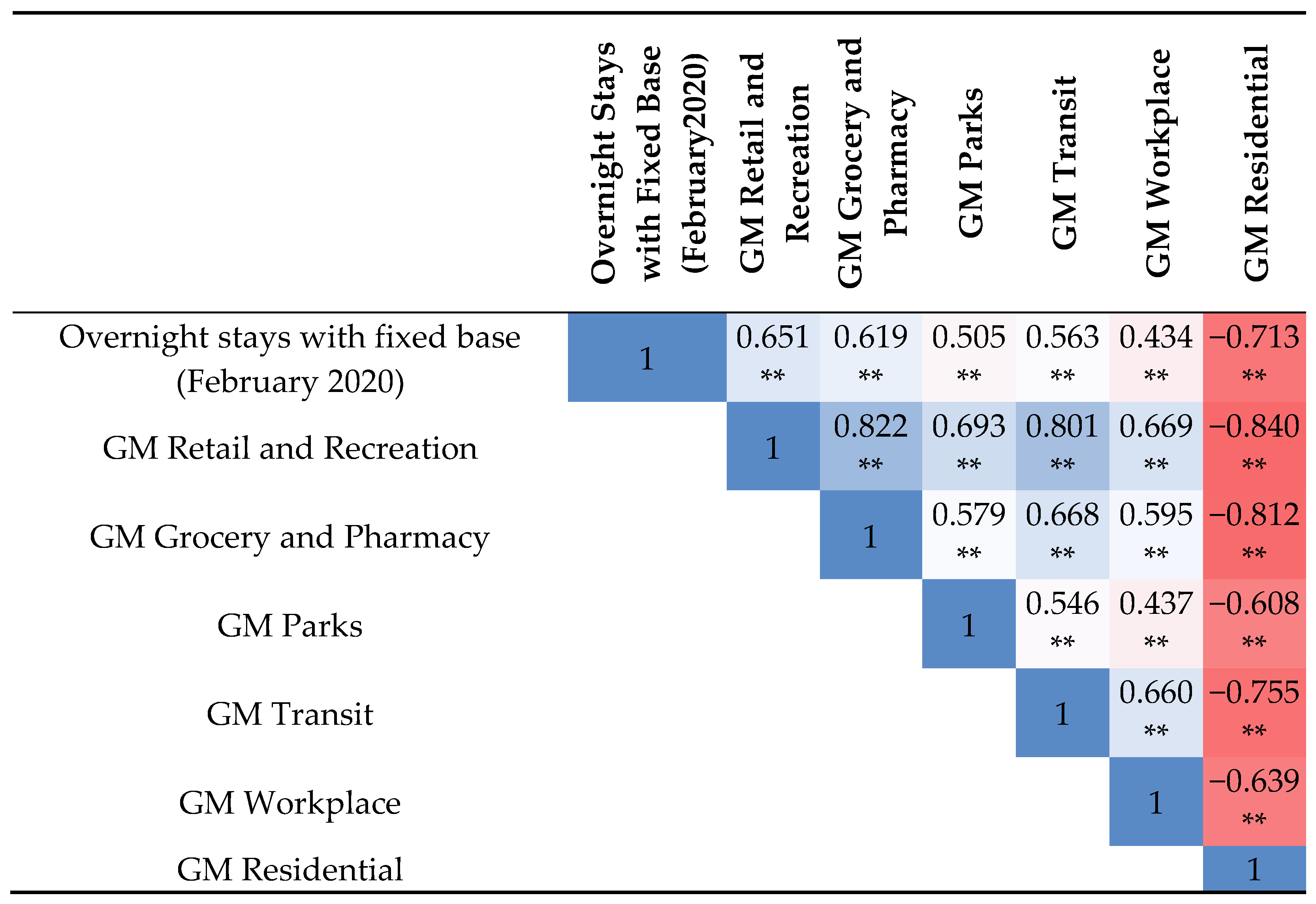
• The Spearman correlation to analyze the direction, power, and statistical significance of the association between variables, respectively, of all the GM6 and overnights for the monthly data of 41 Romanian counties. The heat map was used for a better visualization of the correlations (Figure 2 from the next section).
• An overall regression model (with collinearity analysis/statistics) with Enter and Forward methods applied to all mobility indices, as independent variables, and overnights as a fixed base index dependent variable, to determine/find the best and statistically significant predictors of Romanian tourism during the pandemic;
• A group of methods using all the mobility indicators (GM6), respectively:

  a.

  Factor analysis (PCA—Principal Component Analysis with Varimax rotation) to reduce the 6 variables (GM6 indices) to a smaller number of factors that explain a significant percentage of the total variance (at least 70%) and to determined, for the pandemic era, how mobility indicators were grouped and which of them better explained the total variance, overall, for Romania; those selected remained in the study;

  b.

  A specific regression model with Enter and Forward methods using the factors from factorial analysis (PCA) as independent variables and overnights as fixed base index dependent variable to validate (or not) the overall regression model used in point 5.

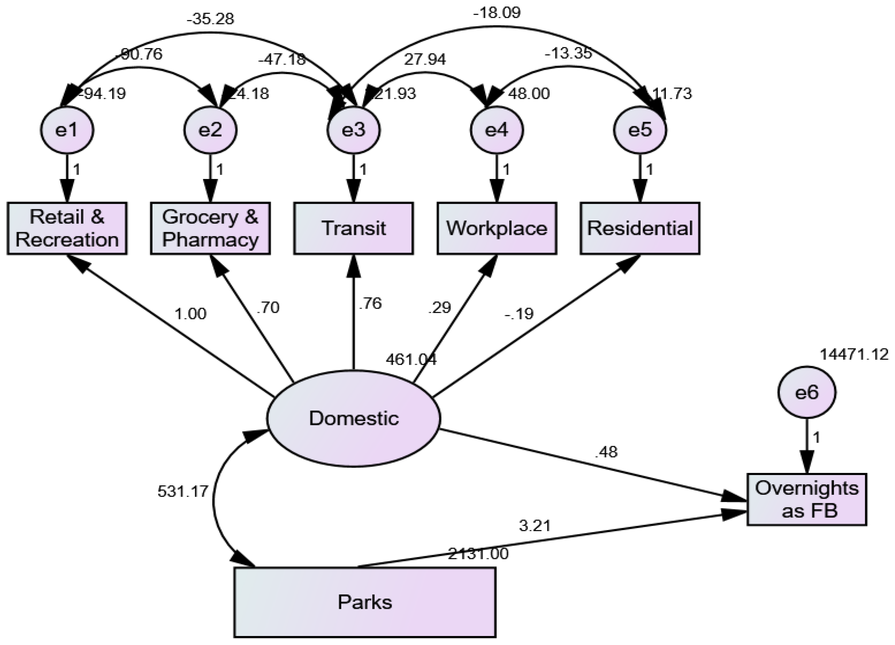
• Structural Equation Model (SEM) framework with SPSS—AMOS software was used to investigate the direct and indirect effects of independent variables, the Google Mobility data [33], on the dependent variable (overnight stays, as a fixed base for February 2020) considering the intervening effects of the mediators. This method was used by Rahman et al. [33] at the early stage of the pandemic to find a pattern in changing mobility of people from 88 countries around the world, and we used this method for all 41 counties (and Bucharest) of Romania. Rahman et al. [33] used only four of the six Google Mobility data dimensions, respectively: retail and recreation, transit, workplace, and residential, without parks, and grocery and pharmacy.

For statistical analyses, SPSS 23.0 (licensed), Microsoft Excel, and AMOS Graphics 22.0 (licensed) were used. The statistical methods from the above-mentioned points 4 and 5 analyzed which of the Google dimensions are more associated and better predict one of the most important indicators in tourism, overnight stays. We opted for regression models as predictor identifiers due to the systematic review of big data-based urban locations made by Kong et al. [45], who mention regression models as one of the most used methods for big data analysis in the research of Atalay and Solmazer [46].

3. Results and Discussions

In this paragraph, we present the results of the specific analysis for Romania at the national level, using only the Google Mobility indices, collected for all 41 Romanian counties and Bucharest. The Apple Mobility indices are not reported in detail for each county; therefore, we decided not to include these in the study. To measure the tourism activity during the same period (March 2020–April 2021), we also used the overnight stays (number) and the overnight stays with a fixed base (with February 2020 as the fixed base). The descriptive statistics at the national level are presented in the

Table 2. Descriptive statistics for research variables.

		Overnight Stays with Fixed Base (February 2020)	GM Retail and Recreation	GM Grocery and Pharmacy	GM Parks	GM Transit	GM Workplace	GM Residential
N	Valid	588	588	588	588	588	588	588
	Missing	0	0	0	0	0	0	0
Mean		−12.0848	−20.6341	−2.7355	−0.6163	−18.4154	−22.3845	3.3875
Median		−43.0650	−20.8750	−0.5100	−10.5150	−20.0050	−20.5300	2.1600
Mode		−97.08	−31.19	−36.87	−18.10	−36.52	−18.55	−0.97
Std. Deviation		195.4267	19.16961	14.21939	46.20203	21.92626	9.33088	5.32048
Minimum		−99.90	−73.50	−50.77	−76.70	−71.37	−58.77	−4.93
Maximum		2765.38	66.06	45.13	643.67	101.53	0.00	24.33
Percentiles
25		−66.7625	−30.7250	−10.8250	−23.5875	−31.2250	−26.1150	−0.7475
50		−43.0650	−20.8750	−0.5100	−10.5150	−20.0050	−20.5300	2.1600
75		−15.3875	−9.3550	6.1300	10.7300	−7.3300	−15.9000	6.4450

(Source: own calculations).

.

From the above data, it is observed that, on average, at the level of Romanian counties, the largest decreases in Google mobility indices were registered for Google mobility workplace (−22.4%), Google mobility retail (−20.6%), and Google mobility transit (18.4%). The only positive evolution is for Google Mobility Residential (+3.4%).

Regarding the overnight stays as a fixed base index (February 2020), at the level of the Romanian counties, there was an average decrease of 12.08%, the mode being 97.08%, but with very large standard deviations from the average (±43.06%). Analyzing the percentiles, only 25% of the counties registered decreases in the overnight stay index below 67%, half of them (median) having a decrease below 43%.

The time series for the period of March 2020–February 2021, for all the variables from the research, are presented in the Figure 2, along with the trendline for overnights as a fixed base for February 2020.

The Explore Outliers analysis points out that according to (

Table 3. Extreme values.

Overnights as Fixed Base Index (February 2020)					Google Mobility Parks			Google Mobility Retail and Recreation			Google Mobility Residential
		Case Number	County	Value	Case Number	County	Value	Case Number	County	Value	Case Number	County	Value
Highest	1	224	Constanța	2765.38	224	Constanța	643.67	224	Constanța	66.06	84	Municipiul București	24.33
	2	182	Constanța	2180.56	182	Constanța	470.57	182	Constanța	63.03	67	Ilfov	23.67
	3	248	Tulcea	1699.36	266	Constanța	151.75	248	Tulcea	43.31	55	Cluj	21.63
	4	206	Tulcea	1256.62	231	Harghita	150.50	206	Tulcea	34.52	79	Timiș	20.67
	5	290	Tulcea	1026.23	248	Tulcea	140.56	221	Caraș−Severin	31.00	50	Brașov	20.03
Lowest	1	73	Prahova	−99.90	84	Municipiul București	−76.70	84	Municipiul București	−73.50	293	Vrancea	−4.93
	2	50	Brașov	−99.89	50	Brașov	−61.83	55	Cluj	−73.43	258	Bistrița	−4.87
	3	82	Vâlcea	−99.87	76	Sibiu	−57.13	77	Suceava	−70.93	272	Gorj	−4.73
	4	112	Mureș	−99.86	79	Timiș	−56.03	50	Brasov	−69.90	259	Botoșani	−4.67
	5	70	Mureș	−99.86	159	Sălaj	−53.93	66	Iași	−69.70	282	Olt	−4.63

(Source: authors’ own calculations).

), the highest values for overnight stays were for the Danube Delta and the Black Sea seaside (Constanța and Tulcea counties). The lowest values for overnights belonged to Brașov, Mureș, Prahova, and Vâlcea, counties that usually are the most visited outside of the pandemic era. The highest values for Google mobility parks emphasized counties like Constanța, Harghita, and Tulcea; the lowest values belonged to the Romanian capital Bucharest, as well as Brașov, Sibiu, Timiș, and Sălaj. The highest values for Google mobility retail and recreation are from Constanța, Tulcea, and Caraș Severin, and the lowest values were for Bucharest, Cluj, Suceava, and Brașov Iași; the counties boasting the bigger malls and larger number of retailers. For variable Google mobility residential, the highest values belong to Bucharest, Ilfov (near to Bucharest), Cluj, Timiș, and Brașov. The lowest values for this mobility data are from the following counties: Vrancea, Bistrița, Gorj, Botoșani, and Olt.

We tested the normality of the data distribution with the One-Sample Kolmogorov–Smirnov test using Lilliefors significance correction. None of the eight variables from the study registered a normal distribution for the analyzed period, which is explained by the continuous adaptation of the restriction measures related to mobility, more accentuated at the beginning of the period (lockdown in March 2020) and adapted according to the evolution of the incidence rate for each county.

The Spearman’s rho correlation coefficients are presented in the following heat map (Figure 3), and the statistically significant value are marked (red color for negative correlations and blue color for positive correlations).

According to the results from Figure 3, it can observe that:

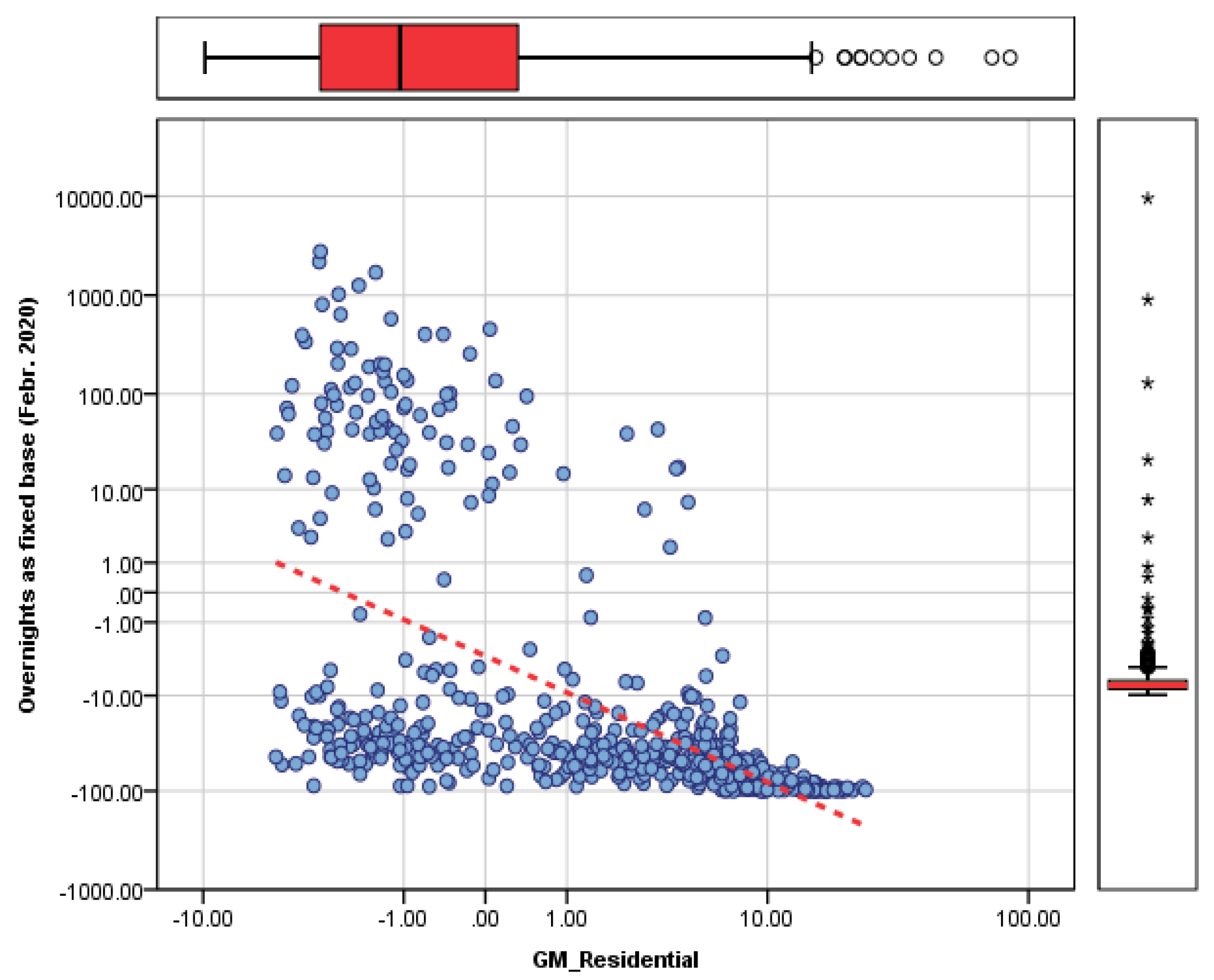
• The GM residential data negative correlates with all the GM indicators and overnights as a fixed base index. The highest value is between GM residential and GM retail and recreation (−0.840), follow by GM residential and GM grocery and pharmacy (−0.812); this means that all the Google Mobility data that measures the movement of people during the pandemic and exhibits strong negative correlations between these indices. Additionally, there are strong negative correlations between GM residential and overnights (−0.713) and between GM residential and GM transit (−0.755).
• There are strong positive (direct) correlations between GM grocery and pharmacy and GM retail and recreation (+0.822), and between GM transit and GM retail and recreation (+0.801).
• There is positive correlation, with a medium to strong intensity, between GM parks and GM retail and recreation (+0.693), GM retail and recreation and overnights (+0.651), GM workplace and GM retail and recreation (+0.669), and GM transit and GM grocery and pharmacy (+0.668).
• There is a medium intensity, positive correlation, between: overnights and GM grocery and pharmacy (+0.619), overnights and GM transit (+0.563), GM grocery and pharmacy and GM parks (+0.619), and GM grocery and pharmacy and GM workplaces (+0.595).

To analyze which of the six Google Mobility indices is the best predictor for overnight stays (as a fixed base index), we used the multilinear regression model in three variants:

• Model 1, with all six Google Mobility indices as independent variables and the overnight stays (as a fixed base index) as the dependent variable by using the enter method for the regression model;
• Models 2–4, with all six Google Mobility indices as independent variables and the overnight stays (as a fixed base index) as the dependent variable by using the forward method for the regression model;
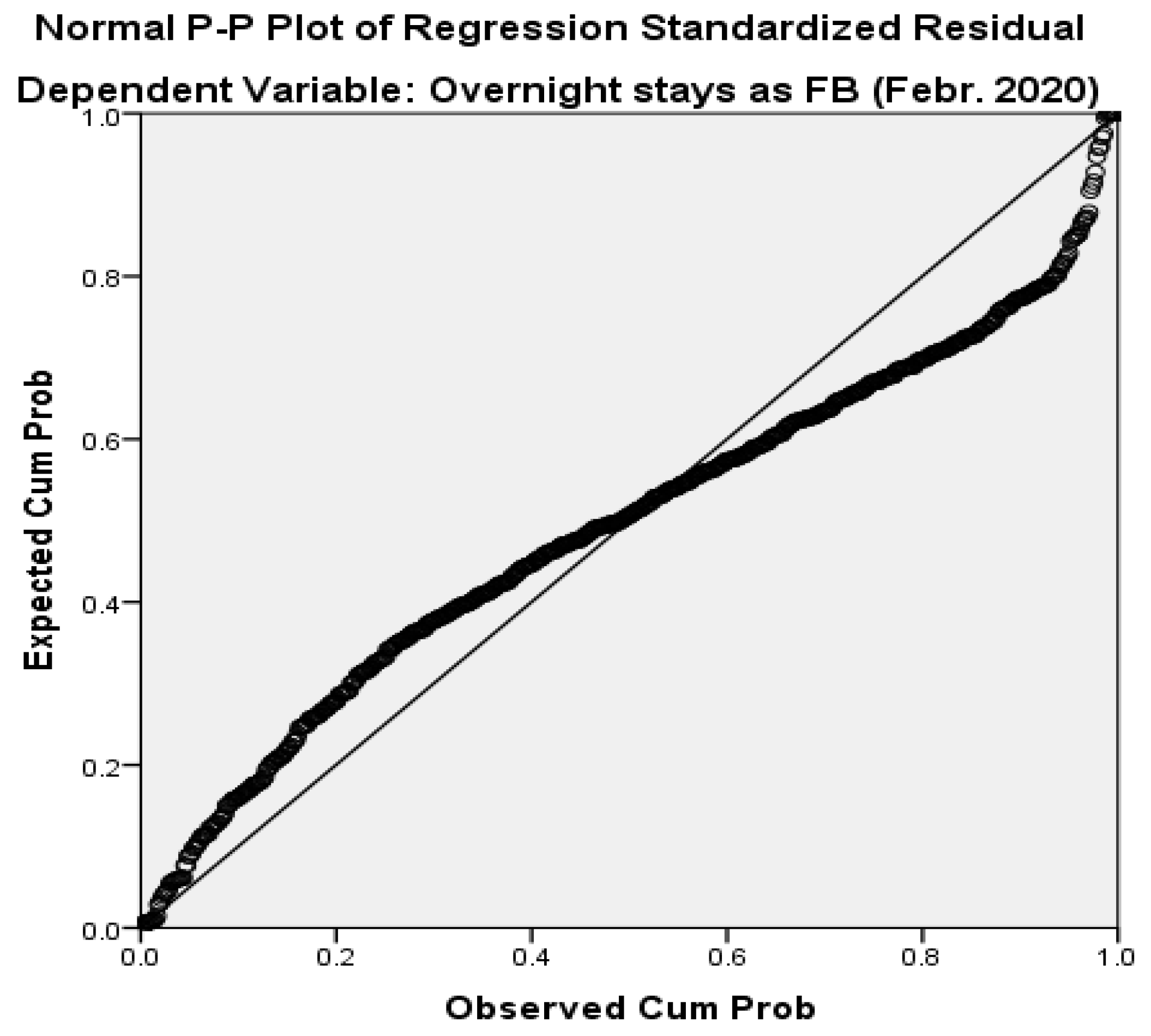
• Model 5, with two factors resulted from factorial analysis (PCA with Varimax rotation and Kaiser normalization) as independent variables and the overnight stays (as a fixed base index) as the dependent variable.

For Model 1 (enter method), the R2 coefficient is 0.636; for models 2–4, using the forward method, the R2 coefficients are: 0.618, 0.623, and 0.635. The ANOVA results indicate statistical significance for all models, ranging from 1 to 4 (p-value = 0.000), for both the enter and forward methods. The multicollinearity test indicates no collinearity, all VIF values being between 1 and 10. The standardized beta coefficients for Model 1 are presented in

Table 4. Coefficients for Models 1–4.

Model		Unstandardized Coefficients		Standardized Coefficients	t	Sig.	Collinearity Statistics
		B	Std. Error	Beta			Tolerance	VIF
1 *	(Constant)	4.711	17.754		0.265	0.791
	GM_ Retail and Recreation	2.044	0.699	0.201	2.925	0.004	0.133	7.505
	GM_Grocery and Pharmacy	0.911	0.757	0.066	1.203	0.229	0.206	4.844
	GM_Parks	3.105	0.148	0.734	21.048	0.000	0.515	1.941
	GM_Transit	0.234	0.343	0.026	0.682	0.496	0.422	2.367
	GM_Workplace	0.045	0.885	0.002	0.050	0.960	0.351	2.847
	GM_Residential	10.363	2.148	0.282	4.825	0.000	0.183	5.456
2 **	(Constant)	−10.035	4.983		−2.014	0.044
	GM_Parks	3.326	0.108	0.786	30.819	0.000	1.000	1.000
3 **	(Constant)	−19.125	6.055		−3.159	0.002
	GM_Parks	3.462	0.119	0.818	29.041	0.000	0.812	1.232
	GM_Residential	2.708	1.035	0.074	2.616	0.009	0.812	1.232
4 **	(Constant)	11.671	9.220		1.266	0.206
	GM_Parks	3.091	0.145	0.731	21.351	0.000	0.534	1.873
	GM_Residential	8.955	1.753	0.244	5.108	0.000	0.274	3.644
	GM_ Retail and Recreation	2.529	0.578	0.248	4.379	0.000	0.195	5.132

Notes: * enter method; ** forward method. (Source: authors’ own calculations).

.

The regression model shows, based on unstandardized coefficients values, shows (Equation (1)):

• upon increasing with 1 unit of GM_Parks, the overnights increase with 3.105,
• upon increasing with 1 unit of GM_ Retail and Recreation, the overnights increase with 2.044
• upon increasing with 1 unit of GM_ Residential, the overnights increase with 10.363.

We will correct the mathematical sign in the regression equation, since all the means are negative (Table 3), and only the GM residential is positive. Moreover, the GM residential data is powerfully negatively correlated with all variables in the study (Figure 3). Therefore, the correct regression equation is presented as follows, based on Model 1 using the enter method, Equation (1), and Model 4 using the forward method, Equation (2):

Overnights as fixed base index (Febr. 2020) = 11.671 + 2.044 GM_ Retail and Recreation + 0.911 GM_Grocery and
Pharmacy + 3.091 GM_Parks + 0.234 GM_Transit + 0.045 GM_Workplace − 10.363 GM_Residential

(1)

Overnights as fixed base index (Febr. 2020) = 11.671 + 3.091 GM_Parks + 2.529 GM_ Retail and Recreation −
8.955 GM_Residential

(2)

The histogram (Figure 4), the normal P-P plot (Figure 5), and the regression residual plot—homoscedasticity and linearity (Figure 6) are presented below.

As shown in Table 4, three of the six Google Mobility indices are good predictors and are statistically significant for overnight stays as a fixed base (February 2020), in order of importance according to values of the standardized beta coefficients and based on the relative strengths of our predictors:

• Google Mobility Parks (p-value = 0.000, standardized beta coefficients = 0.734),
• Google Mobility Residential (p-value = 0.000, standardized beta coefficients = 0.282), and
• Google Mobility Retail (p-value = 0.004, standardized beta coefficients = 0.201).

Figure 7, Figure 8 and Figure 9 represent the regression line for each of the statistically significant predictors for overnights as a fixed base for Romania during March 2020–April 2021, with the dependent variable increasing in regards to the Google Mobility parks and Google Mobility retail and recreation and decreasing in regards to Google Mobility residential. Figure 10 presents the scatter plots for overnights as the dependent variable and Google Mobility parks as the independent variable for each month to emphasize that during the well-known time for holidays, the variations of overnights are explained regarding GM parks as follows: for April 2020, 37% (R² = 0.368), for July 2021, 78% (R² = 0.781), and for August 2021, 72% (R² = 0.716), according to data from Figure 10.

By applying the factorial analysis (PCA), the total variance explained by the Google Mobility indices is 84.75%, but we chose the number of factors (principal components) manually. The rotated component matrix is presented in Table 5, and the component plot is shown in Figure 11. Thus, according to these:

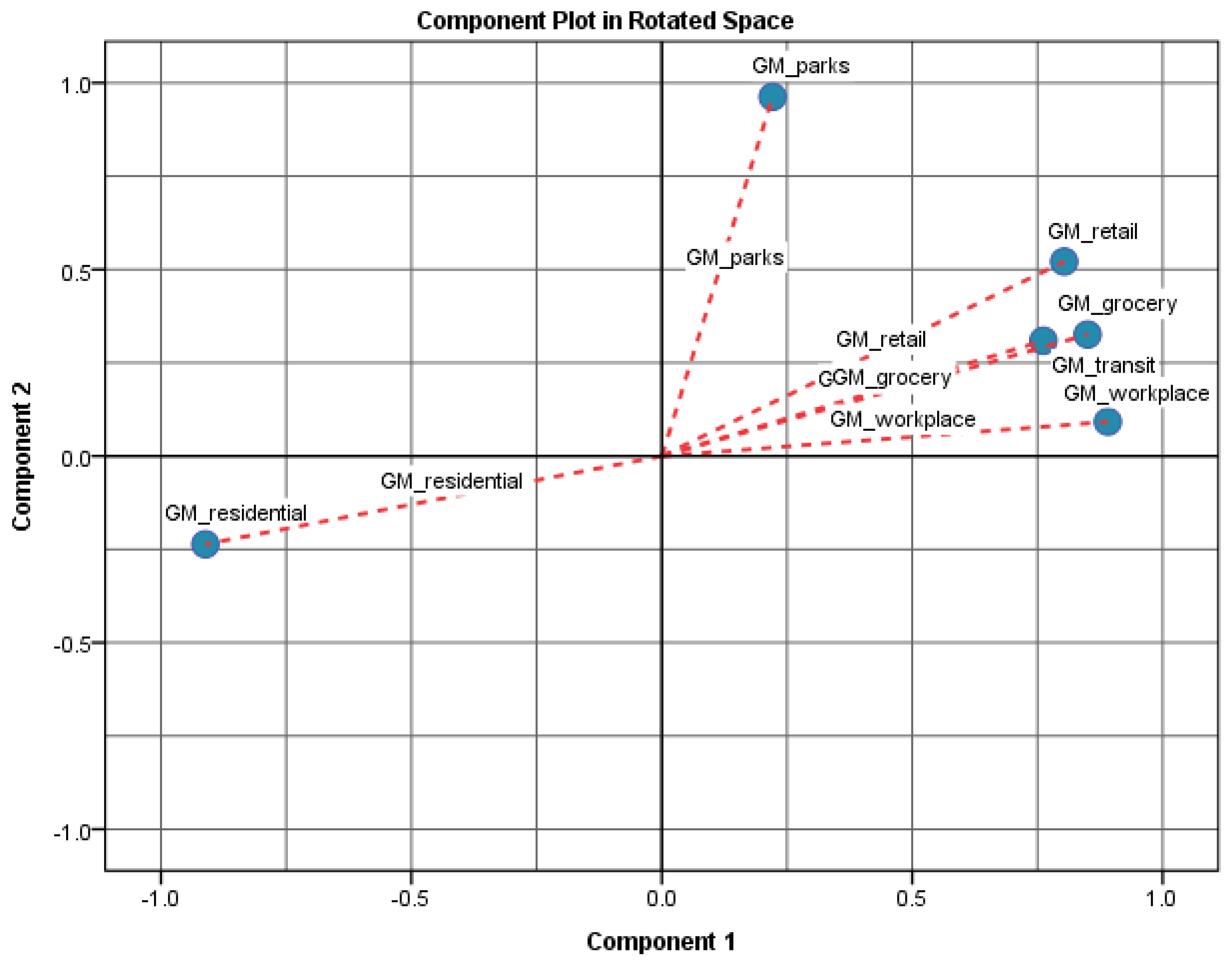
• The principal component PC1 includes five of six Google Mobility indices: Google Mobility residential, Google Mobility workplace, Google Mobility grocery and pharmacy, Google Mobility retail and recreation, and Google Mobility transit. These factors explain 60.34% of the total variance;
• The principal component PC2 includes only one index, Google Mobility Parks and explains 24.4% of the total variance.

Table 5. Rotated Component Matrix ^a.

	Component
	PC1	PC2
Google Mobility Residential	−0.911	−0.236
Google Mobility Workplace	0.891	0.092
Google Mobility Grocery and Pharmacy	0.850	0.326
Google Mobility_ Retail and Recreation	0.803	0.521
Google Mobility_Transit	0.762	0.309
Google Mobility_Parks	0.221	0.963

(Source: authors’ own calculations). Note: a. Rotation converged in 3 iterations; Extraction Method: Principal Component Analysis; Rotation Method: Varimax with Kaiser Normalization ^a.

Table 5. Rotated Component Matrix ^a.

	Component
	PC1	PC2
Google Mobility Residential	−0.911	−0.236
Google Mobility Workplace	0.891	0.092
Google Mobility Grocery and Pharmacy	0.850	0.326
Google Mobility_ Retail and Recreation	0.803	0.521
Google Mobility_Transit	0.762	0.309
Google Mobility_Parks	0.221	0.963

(Source: authors’ own calculations). Note: a. Rotation converged in 3 iterations; Extraction Method: Principal Component Analysis; Rotation Method: Varimax with Kaiser Normalization ^a.

Figure 11. Component plot in rotated space.

Figure 11. Component plot in rotated space.

The second regression model, Model 5, has a good value for R² (0.621), and the ANOVA test indicated that Model 5 is statistically significant (p-value = 0.000). The values for standardized beta coefficients are presented in

Table 6. Coefficients for Model 2.

Model		Unstandardized Coefficients		Standardized Coefficients	t	Sig.
		B	Std. Error	Beta
5	(Constant)	−12.085	4.972		−2.430	0.015
	PC1	28.243	4.976	0.145	5.675	0.000
	PC2	151.349	4.976	0.774	30.413	0.000

(Source: authors’ own calculations).

.

In the case of Model 5, we conclude that the second factor (PC2), consisting of the Google Mobility Parks index is, in fact, the best predictor for overnight stays as a fixed base index, with an appropriate value of standardized beta coefficient like that in the Model 1 (0.774), and alone explaining one-quarter of the total variance. The model shows that when increasing with 1 unit of PC2 (Google Mobility Parks), the overnights increase by 151.349 units, and when increasing with 1 unit of PC1, the overnights increase by only 28.243 units.

For the Structural Equation Model (SEM), we proposed the following variables:

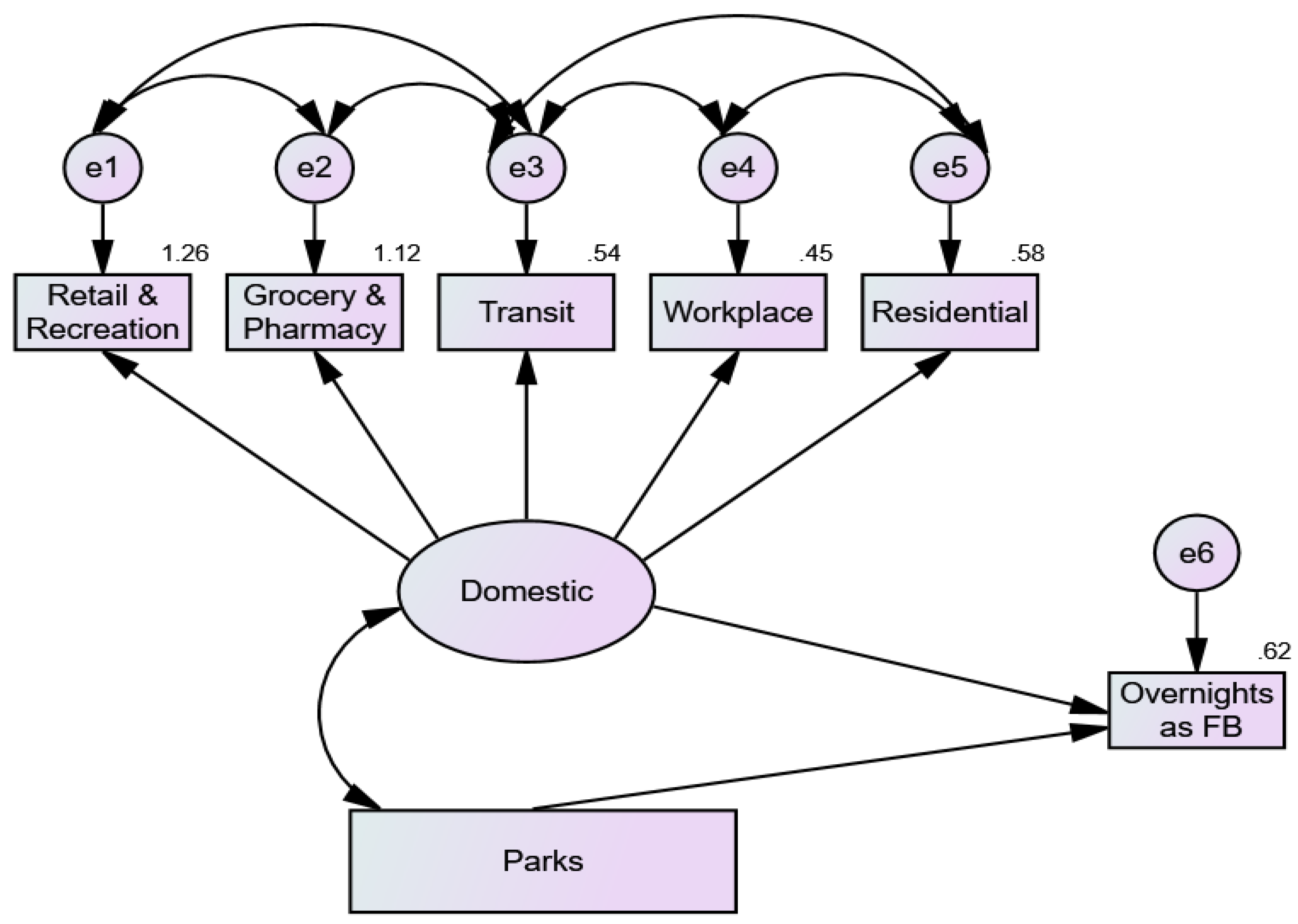
• Five observed, endogenous variables of the model: overnight stays as a fixed base, Google Mobility retail and recreation, Google Mobility grocery and pharmacy, Google Mobility transit, Google Mobility workplace, and Google Mobility residential, are, in fact, the variables that composed the PC1 factors from the above analysis and the dependent variable in the regression models;
• One observed, exogenous variable of the model: Google Mobility parks;
• Seven unobserved, exogenous variables: e1–e6 and
• Domestic.

The unstandardized estimates model from the SEM is presented in Figure 12, and the standardized model is shown in Figure 13.

The hypothesis for the chi-square statistics is the reduced model (overidentified); this fits the data, as does the just-identified (full, saturated) model. The results of SEM by using AMOS 22.0 software indicate that the chi-square statistic for the estimated model is 107.694, df = 7 and p = 0.000. The unstandardized coefficients (estimate) and significant regression paths (P) are presented in

Table 7. Regression Weights and Squared Multiple Correlations.

			Unstandardized				p (Bias-Corrected)	Squared Multiple Correlations
			Estimate	S.E.	C.R.	p			Estimate (Standardized)
Retail and Recreation	<---	Domestic	1.000				….
Grocery and Pharmacy	<---	Domestic	0.700	0.018	39.135	***	0.002	Overnights_as BF (Febr. 2020)	0.620
Transit	<---	Domestic	0.755	0.053	14.248	***	0.020	Residential	0.585
Workplace	<---	Domestic	0.291	0.017	17.203	***	0.008	Workplace	0.448
Residential	<---	Domestic	−0.189	0.010	−19.204	***	0.012	Transit	0.542
Overnights as BF (Febr. 2020)	<---	Domestic	0.483	0.202	2.390	0.017	0.242	Grocery and pharmacy	1.120
Overnights_as BF (Febr. 2020)	<---	Parks	3.206	0.119	26.959	***	0.006	Retail and Recreation	1.257

(Note: *** = p < 0.001). (Source: authors’ own calculations).

, based on the maximum likelihood estimates method. The results show that all the regression paths are statistically significant for p < 0.05 for the unstandardized model.

As Figure 13 indicates, the total effects are explained only through direct effects (standardized), with no intervening variables involved, as follows:

• The cumulative direct effect of the latent variable Domestic and Google Mobility parks on overnight stays as a fixed base (February 2020) indicates a value for path coefficient = 0.620;
• The direct effect of the latent variable Domestic is (1.257) × (1.120) × (0.542) × (0.448) × (0.585) = 0.199;
• The direct effect of mobility data Google Mobility parks is (0.620–0.199) = 0.421.

Based on the results from Table 7, column P (bias-corrected), the direct effect of the latent variable Domestic is not statistically significant (p = 0.242).

Table 8. Goodness-of-Fit Statistics for SEM.

	CMIN					RMR, GFI
Model	NPAR	CMIN	DF	p	CMIN/DF	RMR	GFI	AGFI	PGFI
Default model	21	107.694	7	0.000	15.385	67.943	0.954	0.816	0.239
Saturated model	28	0.000	0			0.000	1.000
Independence model	7	3713.227	21	0.000	176.820	1444.002	0.301	0.068	0.226
	Baseline Comparisons					RMSEA
	NFI Delta1	RFI rho1	IFI Delta2	TLI rho2	CFI	RMSEA	LO 90	HI 90	PCLOSE
Default model	0.971	0.913	0.973	0.918	0.973	0.157	0.131	0.183	0.000
Saturated model	1.000		1.000		1.000
Independence model	0.000	0.000	0.000	0.000	0.000	0.547	0.533	0.562	0.000

(Source: authors’ own calculations).

presents the goodness of fit statistics for the estimated model.

The results from Table 8 indicate a satisfactory estimated model using structural equation modeling as follows (values in bold and italics in Table 8):

• CMIN (chi-squared statistic) is 107.694, and CMIN/DF (the relative chi squared) is 15.385; this means that the fit of data is reduced by only 15% by dropping one or more paths;
• The goodness-of-fit index (GFI) is 0.954 > 0.9, and the adjusted goodness of fit (AGFI) is 0.816, being relatively close values;
• The PGFI (parsimony GFI) of the independent model is lower than PGFI of the default model (0.226 < 0.239);
• The normed fixed index (NFI) is 0.971 > 0.95, indicating a good fit of the estimated model;
• The comparative fit index (CFI) is 0.973 > 0.95 and the Tucker–Lewis index is 0.918 > 0.95, indicating a relatively good model data fit, in general;
• The root mean square error of approximation (RMSEA) is 0.157, with the lower value for the 90% confidence interval (LO 90) = 0.131 and an upper value for the 90% confidence interval (HI 90) = 0.183; this means only a 16% lack of fit when compared to the saturated model.

4. Summary and Conclusions

The present research results pointed out that there is a good and determinant relationship between the domestic travel of the Romanian tourists, reflected in their real time smartphone signals and gathered statistical data from tourism service providers, hotels, and other accommodations and/or services. The present research related the observational data from Google, obtained from smartphone location tracking technologies of its providers, from all the Romanian counties and Bucharest, during the pandemic months during 2020–2021, with tourism overnights for these locations. While biases exist in populations with Google Location History (GLH) data, smartphones are making these mobility data increasingly appropriate for a wide range of scientific questions [47]. The aim of this research was to analyze the existence or not of a powerful/moderate/poor and stable relationship between these two types of data, throughout all Romanian locations and different seasonal situations.

For domestic tourism regarding all 41 counties and Bucharest, we found strong and moderate to strong correlations between: Google Mobility retail and recreation and Google Mobility grocery and pharmacy, Google Mobility retail and recreation and Google Mobility transit stations (strong correlations, statistically significant), but also between the overnights stays and Google Mobility retail and recreation, overnights stays and Google Mobility grocery and pharmacy, and overnights stays and Google Mobility transit stations (moderate correlations, statistically significant). The Google Mobility residential data correlates negatively and strongly with all other dimensions, signaling that when people stay at home, they are not outdoors, so the residential data is also reliable. These results, completed using outlier exploratory analysis, offer an answer regarding the destinations preferred by the Romanian tourists during the COVID-19 pandemic; the highest values indicated the preference for the Danube Delta and the Black Sea seaside, as well as counties with national parks or a good infrastructure for leisure activities (such as Harghita County). During the COVID-19 pandemic, large and developed Romanian counties with good infrastructures of malls and retail businesses were affected, recording the lowest values of mobility for retail and recreation areas such as Bucharest, Cluj, Brașov, Iași, and Suceava counties, due of highest number of restrictions and lockdowns being recorded here.

The regression models applied in the research to determine which of the six Google Mobility dimensions are good predictors for overnight stays at the county level in Romania emphasize that the best statistically significant predictor (not collinear with variables) is Google Mobility parks, follow by Google Mobility residential and Google Mobility retail and recreation. Outside of the COVID-19 pandemic the transportation and tourism dimensions are co-dependent because there would be no tourism without supporting transportation [48], but our results emphasize that the COVID-19 pandemic changed the behavior for travel, in general, and for tourism specifically, and therefore, the GM transit is not a good predictor for tourism, showing moderate correlation with overnight stays for Romania at the county level.

The second regression model, with the factors (principal components) resulted from PCA as independent variables and overnight stays as the dependent variable, confirmed the previous results, respectively, that for Romania, during the COVID-19 pandemic, the best predictor is Google Mobility parks. Our methodological approach confirms the results of Garcia-Cremades et al. [49] by using multivariate analysis for forecasting changes. Moreover, our research results from the regression models show the direction of the mobility behavior of people and/or tourists during the COVID-19 pandemic, out of restrictive areas (retail, grocery, pharmacy, transit, workplace), with a latent behavior toward local and/or national parks, public beaches, etc.

By using structural equation modeling, we investigated the causal relationship (direct and/or indirect) between Google Mobility data and observed data through the latent variable, called Domestic, and Google Mobility parks, through overnight stays with a fixed base (for February 2020). The results indicate a goodness of fit estimated model that indicate the direct and determinant effect of Google Mobility parks on tourism and leisure activities in Romania during COVID-19 for the first 14 months of pandemic.

Collectively, the key findings of the study are that the domestic or routine activities, such as going to the workplace or grocery shopping, are not at all, or only weakly, related to tourism. The residential function is connected strong, but inversely to tourism, which is evident, (when people are home, they do not travel). However, for some partly domestic activities, such as retail shopping and recreation, transit can sometimes be linked with tourism (of course, this might depend on the commercial culture of the place observed). The most related factor is the parks, although this can also be an urban activity (because Google collects data from urban parks as well).

In the international literature, we found that only the Google trends information offered significant benefits to forecasters; particularly regarding tourism [25], the novelty of the authors’ contributions consisted of proving that mobility dimensions, such as Google Mobility parks, could be, during an atypical time such as the COVID-19 pandemic, a good predictor for domestic tourism, but it is important to continue the research and extend the time series used in the study to analyze the post-pandemic mobility of tourists using the Google Mobility dimensions. Therefore, we consider that our results confirmed the results of Souza et al. [28] showing the global trend of declining public interest in national parks during the initial phase of the COVID-19 pandemic, with considerable variation between both parks and countries [28]. The Romanian tourists reoriented during the pandemic, not to inside leisure and socialization activities, measured by Google Mobility retail and recreation (restaurants, museums, theme parks, etc.), but to outside leisure, tourism, and social activities, measured by Google Mobility parks, including local and/or national parks, public beaches, public gardens, and all types of activities that could replace classical tourism activities reflected in the increase in overnights stays at each location showing an increase in Google Mobility parks data. Our results are in line with the results of Atalay and Solmazer [46], since we used regression models and discovered that staying at home, and mobility in public spaces, while avoiding retail and recreation sites (marginally significant) were the defining dimensions during April–May 2020.

The tourism activities imply a strong social component, which was disrupted during the COVID-19 pandemic. Our results confirm the results of Jensen [50] and Pramana et al. [26], which showed the actual integration of the Internet in the “real world,” and that it is included as a part of the users’ social space due to the constant dynamics between physical, imaginary, and mediated experiences, especially regarding tourism.

Moreover, travel and tourism activities are directly linked to people’s personal, mental, and social well-being (PMS well-being) [51], aspects pushed aside during COVID-19 pandemic; therefore, our research results emphasized and confirmed the determinant relationship between travel, leisure, and tourism activities and the PMS well-being [51] of Romanian tourists.

Regarding the results inferred from outside research, this study also confirms the Pramana et al. [26] study results showing that the big data sources, such as Google Mobility data, are shown to be a good proxy to infer the impact of the pandemic on domestic tourism, despite the unpredictability of human behavior during the COVID-19 pandemic [49]. The results from this study could help explain the mobility patterns of park visits during the pandemic and predict the process of returning to normal. Following the expiration of stay-at-home orders, a single metric of mobility was not sensitive enough to capture the complexity of human interactions [52]. Monitoring mobility can be an important tourism mobility trend and public health tool, but it should be modeled as a multidimensional construct [52], linked to other variables which are directly linked to tourism activities. The COVID-19 pandemic not only reduced tourism activity, but also the physical activity level of the population [39], including the walking level [39].

Our research results confirm the results of Park et al., [53] on big data regarding tourism, which concluded that the COVID-19 pandemic substantially reshaped the tourism and hospitality industries, but studies on the changes in travel behavior in response to the pandemic are limited [53].

The limits of the research are linked to:

• The problem of including other dimensions in Google, such as shopping, transit travels, etc., that cannot be split, separated, or extracted to emphasize the precise mobility for tourism motivations; in the future, studying the weight of each included dimensions in Google Mobility data may be an important research step. The results of Yang et al. [54], using only three dimensions (retail and recreation, parks, and transit stations) also demonstrated the mobility reduction in tourism in cities [54]. Gunawan [55] also used only these three GM dimensions and demonstrated that six provinces in Indonesia showing higher visitor length-of-stay and hotel occupancy rates also experienced greater mobility change;
• The problem of data not being available from Apple for all Romanian locations at the county level in order to compare and establish if the Google Mobility dimensions or Apple Mobility data better predict the mobility of tourists;
• The lack of similar research results, at the country level (European or worldwide), with which to compare the present research results regarding the main objective to be able to validate whether or not, according to the statistical methods used in the present research, this can be considerate a good path for the future researcher and stakeholders from tourism industry
• The ambiguity of the nature of the visits and trips shown by the travel location history of people’s smartphones, this being, in our opinion, the biggest limitation of the research due of the complementary activities included in the each of the six Google Mobility dimensions.

For future research, the authors’ intent is to apply other quantitative methods, such as grey relational [56,57,58], or neural network [53] analysis, for example, and to include other important available dimensions for the tourism industry, such as a tourism competitiveness index or other tourism indices, as well as details regarding the impact of the COVID-19 pandemic on the most-visited Romanian counties and regions, such as Brașov, Prahova, Sibiu, Maramureș, Bucovina, the Danube Delta, and the Black Sea beach.

Our research highlights that tourism can also be modeled with specific observational data, which data can be more reliable than statistical (collected) data or the data collected via questioning. This study is a first step in this direction, to show how to transform observational data from other sectors into tourism related information. The absolute advantage of the Google Mobility data is that they are available online, for almost any location in the world, at the city, county, or country level. These findings provide useful insights concerning how the tourism, hospitality, and travel sectors are affected by crisis events [54], and these insights apply equally to the future of urban development, public transportation, and behavioral strategies [59].

References

- Bacoș, I.B.; Gabor, M.R. Tourism economy. Mountain tourism: Quantitative analysis of winter destinations in Romania. Economics 2021, 9, 55–70. [Google Scholar] [CrossRef]
- Bacoș, I.B.; Gabor, M.R. Consumers’ Preferences of Winter Tourist Packages in Romania: A Quantitative Case Study. Ann. Dunarea De Jos Univ. Galati Fascicle I Econ. Appl. Inform. 2020, 26, 157–164. [Google Scholar] [CrossRef]
- Nagy, B. Tourism with No Resources? Acta Universitatis Sapientiae. Econ. Bus. 2019, 7, 5–22. [Google Scholar] [CrossRef] [Green Version]
- National Institute of Statistics (INS). Staying Overnight in the Establishments of Touristic Reception by Counties and Localities. 2021. Available online: http://statistici.insse.ro:8077/tempo-online/#/pages/tables/insse-table (accessed on 2 February 2021).
- World Tourism Organization (UNWTO). Tourism Data Dashboard. 2021. Available online: https://www.unwto.org/tourism-data/unwto-tourism-dashboard (accessed on 2 February 2021).
- Wang, S.; Tong, Y.; Fan, Y.; Liu, H.; Wu, J.; Wang, Z.; Fang, C. Observing the silent world under COVID-19 with a comprehensive impact analysis based on human mobility. Sci. Rep. 2021, 11, 14691. [Google Scholar] [CrossRef]
- Baba, C.A.; Stăncioiu, A.F.; Gabor, M.R.; Alexe, F.A.; Oltean, F.D.; Dinu, A.C. Considerations regarding the effects of COVID-19 on the tourism market. Theor. Appl. Econ. 2020, XXVII, 271–284. [Google Scholar]
- Privitera, D.; Nicula, V. Gastronomic and food tourism as an economic local resource: Case studies from Romania and Italy. GeoJ. Tour. Geosites 2018, 1, 143–157. [Google Scholar]
- Nagy, H.K.X.; Segui, E.A. Experiences of community-based tourism in Romania: Chances and challenges. J. Tour. Anal. Rev. Anál. Tur. 2020, 27, 143–163. [Google Scholar] [CrossRef] [Green Version]
- Mionel, V. (Not so) Dark tourism: The Merry Cemetery in Săpânţa (Romania)—An expression of folk culture. Tour. Manag. Perspect. 2020, 34, 100656. [Google Scholar] [CrossRef]
- Matei, D.; Chiriță, V.; Lupchian, M.M. Governance and tourism resilience during the COVID-19 crisis. Case study Bukovina, Romania. GeoJ. Tour. Geosites 2021, 34, 256–262. [Google Scholar] [CrossRef]
- Herman, G.V.; Wendt, J.A.; Dumbravă, R.; Gozner, M. The role and importance of promotion centers in creating the image of tourist destination: Romania. Geogr. Pol. 2019, 92, 443–454. [Google Scholar] [CrossRef]
- Herman, G.V.; Banto, N.; Caciora, T.; Grama, V.; Ungureanu, M.; Furdui, S.; Buhaș, R.; Buhaș, S. Tourism in Bihor County, Romania. Trends and Prospects. Folia Geogr. 2020, 62, 87–105. [Google Scholar]
- Briciu, A.; Briciu, V.-A.; Kavoura, A. Evaluating How ‘Smart’ Brașov, Romania Can Be Virtually via a Mobile Application for Cultural Tourism. Sustainability 2020, 12, 5324. [Google Scholar] [CrossRef]
- Gica, O.A.; Coros, M.M.; Moisescu, O.I.; Yallop, A.C. Transformative rural tourism strategies as tools for sustainable development in Transylvania, Romania: A case study of Sâncraiu. Worldw. Hosp. Tour. Themes 2021, 13, 124–138. [Google Scholar] [CrossRef]
- Liu, Y.; Chin, W.L.; Nechita, F.; Candrea, A.N. Framing Film-Induced Tourism into a Sustainable Perspective from Romania, Indonesia and Malaysia. Sustainability 2020, 12, 9910. [Google Scholar] [CrossRef]
- Cehan, A.; Iaţu, C.; Eva, M.; Ibănescu, B.; Bulai, M. Territorial dynamics of tourism in Romania: A long-term perspective (1990–2016). Hum. Geogr. 2019, 13, 23–44. [Google Scholar] [CrossRef] [Green Version]
- Domènech, A.; Mohino, I.; Moya-Gómez, B. Using Flickr geotagged photos to estimate visitor trajectories in World Heritage cities. ISPRS Int. J. Geo-Inf. 2020, 9, 646. [Google Scholar] [CrossRef]
- Yang, L.; Wu, L.; Liu, Y.; Kang, C. Quantifying tourist behavior patterns by travel motifs and geo-tagged photos from Flickr. ISPRS Int. J. Geo-Inf. 2017, 6, 345. [Google Scholar] [CrossRef] [Green Version]
- Maeda, T.N.; Yoshida, M.; Toriumi, F.; Ohashi, H. Extraction of tourist destinations and comparative analysis of preferences between foreign tourists and domestic tourists on the basis of geotagged social media data. ISPRS Int. J. Geo-Inf. 2018, 7, 99. [Google Scholar] [CrossRef] [Green Version]
- Zhu, X.; Sun, T.; Yuan, H.; Hu, Z.; Miao, J. Exploring group movement pattern through cellular data: A case study of tourists in Hainan. ISPRS Int. J. Geo-Inf. 2019, 8, 74. [Google Scholar] [CrossRef] [Green Version]
- Zaragozí, B.; Trilles, S.; Gutiérrez, A. Passive Mobile Data for Studying Seasonal Tourism Mobilities: An Application in a Mediterranean Coastal Destination. ISPRS Int. J. Geo-Inf. 2021, 10, 98. [Google Scholar] [CrossRef]
- Rodríguez-Echeverría, J.; Semanjski, I.; Van Gheluwe, C.; Ochoa, D.; IJben, H.; Gautama, S. Density-Based Spatial Clustering and Ordering Points Approach for Characterizations of Tourist Behaviour. ISPRS Int. J. Geo-Inf. 2020, 9, 686. [Google Scholar] [CrossRef]
- Lewis, G.K.; Hardy, A.; Wells, M.P.; Kerslake, F.L. Using mobile technology to track wine tourists. Ann. Tour. Res. Empir. Insights 2021, 2, 100022. [Google Scholar] [CrossRef]
- Bangwayo-Skeete, P.F.; Skeete, R.W. Can Google data improve the forecasting performance of tourist arrivals? Mixed-data sampling approach. Tour. Manag. 2015, 46, 454–464. [Google Scholar] [CrossRef]
- Pramana, S.; Paramartha, D.Y.; Ermawan, G.Y.; Deli, N.F.; Srimulyani, W. Impact of COVID-19 pandemic on tourism in Indonesia. Curr. Issues Tour. 2021. [Google Scholar] [CrossRef]
- Perea-Medina, B.; Rosa-Jimenez, C.; Andrade, M.J. Potential of public transport in regionalisation of main cruise destinations in Mediterranean. Tour. Manag. 2019, 74, 382–391. [Google Scholar] [CrossRef]
- Souza, C.N.; Rodrigues, A.C.; Correira, R.A.; Normande, I.C.; Costa, H.C.M.; Guedes-Santos, J.; Malhado, A.C.M.; Carvalho, A.R.; Ladle, R.J. No visit, no interest: How COVID-19 has affected public interest in world’s national parks. Biol. Conserv. 2021, 256, 109015. [Google Scholar] [CrossRef]
- Sadeghvaziri, E.; Rojas, M.B.; Jin, X. Exploring the Potential of Mobile Phone Data in Travel Pattern Analysis. Transp. Res. Rec. J. Transp. Res. Board 2016, 2594, 27–34. [Google Scholar] [CrossRef]
- Google Mobility Data Base. Mobility Report CSV Documentation. Available online: https://www.google.com/covid19/mobility/data_documentation.html?hl=en (accessed on 31 May 2021).
- Google Mobility Reports. Available online: https://support.google.com/covid19-mobility#topic=9822927 (accessed on 31 May 2021).
- Ruktanonchai, C.W.; Lai, S.J.; Utazi, C.E.; Cunningham, A.D.; Koper, P.; Rogers, G.E.; Ruktanonchai, N.E.; Sadilek, A.; Woods, D.; Tatem, A.J.; et al. Practical geospatial and sociodemographic predictors of human mobility. Sci. Rep. 2021, 11, 15389. [Google Scholar] [CrossRef]
- Rahman, M.M.; Thill, J.-C.; Paul, K.C. COVID-19 Pandemic Severity, Lockdown Regimes, and People’s Mobility: Early Evidence from 88 Countries. Sustainability 2020, 12, 9101. [Google Scholar] [CrossRef]
- Tamagusko, T.; Ferreira, A. Data-Driven Approach to Understand the Mobility Patterns of the Portuguese Population during the COVID-19 Pandemic. Sustainability 2020, 12, 9775. [Google Scholar] [CrossRef]
- Irini, F.; Kia, A.; Shannon, D.; Jannusch, T.; Murphy, F.; Sheehan, B. Associations between mobility patterns and COVID-19 deaths during the pandemic: A network structure and rank propagation modelling approach. Array 2021, 11, 100075. [Google Scholar] [CrossRef] [PubMed]
- Ibarra-Espinosa, S.; de Freitas, E.D.; Ropkins, K.; Dominici, F.; Rehbein, A. Negative-Binomial and quasi-poisson regressions between COVID-19, mobility and environment in São Paulo, Brazil. Environ. Res. 2022, 204, 112369. [Google Scholar] [CrossRef] [PubMed]
- Saha, J.; Mondal, S.; Chouhan, P. Spatial-temporal variations in community mobility during lockdown, unlock, and the second wave of COVID-19 in India: A data-based analysis using Google’s community mobility reports. Spat. Spatio-Temporal Epidemiol. 2021, 39, 100442. [Google Scholar] [CrossRef] [PubMed]
- Cot, C.; Cacciapaglia, G.; Sannino, F. Mining Google and Apple mobility data: Temporal anatomy for COVID-19 social distancing. Sci. Rep. 2021, 11, 4150. [Google Scholar] [CrossRef] [PubMed]
- Dobbie, L.J.; Hydes, T.J.; Alam, U.; Tahrani, A.; Cuthbertson, D.J. The Impact of the COVID-19 Pandemic on Mobility Trends and the Associated Rise in Population-Level Physical Inactivity: Insights from International Mobile Phone and National Survey Data. Front. Sports Act. Living 2022, 4, 773742. [Google Scholar] [CrossRef]
- Camba, A.C., Jr.; Camba, A.L. The Effects of Restrictions in Economic Activity on the Spread of COVID-19 in the Philippines: Insights from Apple and Google Mobility Indicators. J. Asian Financ. Econ. Bus. 2020, 7, 115–121. [Google Scholar] [CrossRef]
- Munawar, H.S.; Khan, S.I.; Qadir, Z.; Kouzani, A.Z.; Mahmud, M.A.P. Insight into the Impact of COVID-19 on Australian Transportation Sector: An Economic and Community-Based Perspective. Sustainability 2021, 13, 1276. [Google Scholar] [CrossRef]
- Yang, A.; Yang, J.; Yang, D.; Xu, R.; He, Y.; Aragon, A.; Qiu, H. Human Mobility to Parks Under the COVID-19 Pandemic and Wildfire Seasons in the Western and Central United States. Geohealth 2021, 5, e2021GH000494. [Google Scholar] [CrossRef]
- Yang, Y.; Zhang, C.X.; Rickly, J.M. A review of early COVID-19 research in tourism: Launching the Annals of Tourism Research’s Curated Collection on coronavirus and tourism. Ann. Tour. Res. 2021, 91, 103313. [Google Scholar] [CrossRef]
- Geng, D.C.; Innes, J.; Wu, W.; Wang, G. Impacts of COVID-19 pandemic on urban park visitation: A global analysis. J. For. Res. 2021, 32, 553–567. [Google Scholar] [CrossRef]
- Kong, L.Q.; Liu, Z.F.; Wu, J.G. A systematic review of big data-based urban sustainability research: State-of-the-science and future directions. J. Clean. Prod. 2020, 273, 123142. [Google Scholar] [CrossRef]
- Atalay, S.; Solmazer, G. The Relationship Between Cultural Value Orientations and the Changes in Mobility During the COVID-19 Pandemic: A National-Level Analysis. Front. Psychol. 2021, 12, 578190. [Google Scholar] [CrossRef] [PubMed]
- Ruktanonchai, N.W.; Ruktanonchai, C.W.; Floyd, J.R.; Tatem, A.J. Using Google Location History data to quantify fine-scale human mobility. Int. J. Health Geogr. 2018, 17, 28. [Google Scholar] [CrossRef] [PubMed] [Green Version]
- Miravet, D.; Domènech, A.; Gutiérrez, A. What prompts tourists to become public transportation users at their destination? The case of a Mediterranean city. Travel Behav. Soc. 2021, 24, 10–21. [Google Scholar] [CrossRef]
- Garcia-Cremades, S.; Morales-Garcia, J.; Hernández-Sanjaime, R.; Martínez-España, R.; Bueno-Crespo, A.; Hernández-Orallo, E.; Cecilia, J.M. Improving prediction of COVID-19 evolution by fusing epidemiological and mobility data. Sci. Rep. 2021, 11, 15173. [Google Scholar] [CrossRef] [PubMed]
- Jensen, J.L. Augmentation of Space: Four Dimensions of Spatial Experiences of Google Earth. Space Cult. 2010, 13, 121–133. [Google Scholar] [CrossRef]
- Alipour, H.; Rezapouraghdam, H.; Esmaeili, B. Public Health and Tourism; A Personalist Approach to Community Well-Being: A Narrative Review. Iran. J. Public Health 2020, 49, 447–453. [Google Scholar] [CrossRef]
- Her, P.H.; Saeed, S.; Tram, K.H.; Bhatnagar, S.R. Novel mobility index tracks COVID-19 transmission following stay-at-home orders. Sci. Rep. 2022, 12, 7654. [Google Scholar] [CrossRef]
- Park, S.; Kim, Y.R.; Ho, C.S.T. Analysis of travel mobility under Covid-19: Application of network science. J. Travel Tour. Mark. 2022, 39, 335–352. [Google Scholar] [CrossRef]
- Yang, M.; Han, C.; Cui, Y.; Zhao, Y. COVID-19 and mobility in tourism cities: A statistical change-point detection approach. J. Hospit. Tour Manag. 2021, 47, 256–261. [Google Scholar] [CrossRef]
- Gunawan, N. Community mobility during COVID-19 pandemic and tourism performance: Data mining approach. AIP Conf. Proc. 2022, 2470, 020009. [Google Scholar] [CrossRef]
- Huang, Y.-L.; Lin, C.-T. Constructing grey relational analysis model evaluation of tourism competitiveness. J. Inform. Optim Sci. 2009, 30, 1129–1138. [Google Scholar]
- Maksimović, M.; Urošević, S.; Stanujkić, D.; Karabašević, D. Selection a development strategy of mining tourism based on the Grey relational analysis. Min. Mettalurgy Eng. Bor 2016, 1, 115–124. [Google Scholar] [CrossRef] [Green Version]
- Cheng, Y.-T.; Liang, R.-Q.; Ho, M.-C.; Wu, C.-H. Sensory evaluation of low-carbon city tourism by Grey relational analysis. E3S Web Conf. 2021, 228, 01003. [Google Scholar] [CrossRef]
- Palma, A.; Vosough, S.; Liao, F. An overview of effects of COVID-19 on mobility and lifestyle: 18 months since the outbreak. Transp. Res. Part A Policy Pract. 2022, 159, 372–397. [Google Scholar] [CrossRef] [PubMed]