Abstract
In some scenarios, the log-logistic (LL) distribution is shown to provide the best fit to field measurements in the context of wireless channel modeling. However, a fading channel model based on the LL distribution has not been formulated yet. In this work, we introduce the -distribution as a reformulation of the LL distribution for channel modeling purposes. We provide closed-form expressions for its PDF, CDF, and moments. Performance analysis of wireless communication systems operating under -fading channels is exemplified, providing exact and asymptotic expressions for relevant metrics such as the outage probability and the average capacity. Finally, important practical aspects related to the use of the -distribution for channel fitting purposes are discussed in two contexts: (i) millimeter-wave links with misaligned gain, and (ii) air–ground channels in unmanned aerial vehicle communications.
1. Introduction
The research in stochastic fading models has been intense since the prominent works by Nakagami and Beckmann [1,2]. For decades, fading models arising from the central limit theorem (CLT), such as Rayleigh and Rice ones, have been widely used to model propagation conditions in multipath fading channels for non-line-of-sight (NLOS) and line-of-sight (LOS) conditions, respectively. In those scenarios in which a more sophisticated modeling was required, the Nakagami-m model is usually preferred because of its simple mathematical tractability, compared to other alternatives such as Nakagami-q or Beckmann fading models. With the new century, a number of relevant and more general fading distributions have been proposed [3,4,5,6], which have proven useful to accommodate to a wider set of propagation environments while being supported by empirical evidences.
Still, because of the complex nature of the propagation mechanisms that affect electromagnetic waves, the use of different distributions is required in some scenarios in order to better respond to field measurements. In many cases, the choice of a certain target distribution to model fading channels does not respond to a physically-justified choice of distribution, but instead to convenience. For instance, this is the case of the Weibull distribution, which was proposed in [7,8] as an alternative to model indoor propagation channels because of a reasonable analytical simplicity and its improved fit compared to other alternatives.
In some contexts, the use of the log-logistic (LL) distribution (also known as Fisk distribution) [9,10] has been proposed to model the amplitude or power fluctuations of the signals affected by fading. Several examples include in-body to out-of-body channels [11,12], millimeter-wave cellular networks with misaligned gain [13], scattering caused by foliage [14], air–ground channels in the context of unmanned aerial vehicle (UAV) communications [15,16], underwater optical wireless communications affected by turbulence [17], and others [18,19,20,21]. However, a formal statistical characterization of the LL distribution in the context of wireless channel modeling has not been carried out in the literature, to the best of our knowledge.
In order to fill this gap, and aiming to facilitate the use of the LL distribution for performance analysis purposes, we propose a formulation for the use of the LL distribution in the context of channel modeling, for which the name -distribution is coined. We provide a clear definition of its chief statistics, highlighting its advantages and key differences over other fading channel models. We illustrate that in some cases, the fit provided by the LL distribution may not be associated with a physically plausible fading model, so that caution must be exercised depending on the application. We also exemplify how performance analysis of wireless communication systems operating over -distributed fading channels can be carried out, using standard metrics in communication theory such as the outage probability (OP) and average capacity, and providing simple asymptotic results that shed light on the role of the distribution parameters on system performance.
The remainder of this paper is structured as follows: Section 2 briefly introduces the canonical system model of a wireless communication system. Then, in Section 3, the statistical characterization of the -distribution is described. Applications to performance analysis are given in Section 4, considering the OP and average capacity as metrics of interest, and numerical results are presented. In Section 5, potential inconsistencies when using the -distribution for channel fitting purposed are discussed, whereas the key conclusions are outlined in Section 6.
Notation: Throughout this paper, denotes a probability density function (PDF); is a cumulative distribution function (CDF); denotes the complex Gaussian distribution with parameters (mean) and (variance); denotes the log-logistic distribution with parameters (scale) and (shape); is the expectation operator; the symbol ∼ means statistically distributed as; the symbol ≜ means defined as; and is the sinc function.
2. System Model
Let us consider a canonical wireless communication system, on which a transmitter wishes to communicate with a receiver over a wireless channel. The received signal can be expressed as
where is the available power budget at the transmitter side, encapsulates the gains of the transmit and receive antennas and frequency-dependent propagation losses, d is the distance between the transmitter and the receiver, is the path loss exponent, x is the normalized transmit symbol (i.e., ), represents the additive white Gaussian noise (AWGN) term, and h is a random variable representing the fading channel, which is assumed to be normalized for the sake of convenience, i.e., .
The instantaneous SNR at the receiver side can be represented as
and the average SNR is given by .
3. Statistical Characterization
In this section, we introduce the -distribution to characterize the instantaneous signal-to-noise ratio (SNR) in a fading channel scenario. Specifically, the -distribution is a reformulation of the classical LL distribution, so that one of the parameters of the distribution is explicitly its mean (i.e., its first-order moment). The purpose of this re-parameterization is that the mean value of the physical magnitude that we want to measure, i.e., the SNR in our case, is explicitly defined. We note that, similarly to the case of the log-normal distribution, a power transformation over a -distributed variable results in another -distributed random variable; i.e., if , then . Thus, the -distribution can be used to characterize either the random fluctuations of the fading amplitude , power or SNR. For an -distributed random variable , the PDF is expressed as
where and are the scale and shape parameters of the -distribution, respectively. However, in order to explicitly state the dependence of this distribution with the average SNR, i.e., for the -distribution, we set using the conventional definition of the sinc function. It is worth highlighting that all subsequent evaluations of the sinc function always have an argument lower than unity; thus, such evaluations always yield positive values. With these considerations, the PDF of the -distribution is formally defined as
so that the -distribution has one parameter () besides the average SNR. Hence, it can be encompassed within the class of SNR fading distributions with one shape parameter, similar to the squared versions of Rician, Nakagami-m, Nakagami-q, or Weibull distributions. Similarly to the inverse gamma distribution [22], we note that the first moment of is only defined for . Since the first moment corresponds to the average SNR, this imposes a restriction over the valid range of values for to yield a physically valid fading distribution. Note that the LL distribution is often used for its ability to model a tail behavior heavier than the exponential distribution, which happens only for [10]. Thus, this does not correspond to the range of values for which the -distribution is defined. With all these considerations, the PDF in (4) for the -distribution is defined for and . Hence, the -distribution can be seen as a subset of the classical LL distribution, with the only restriction of for physical reasons. The expression for the CDF of the -distribution is obtained by direct integration of (4), yielding
and the moments are given, for , by
From the expression of the moments, we can compute the amount of fading (AoF) using (6) from its definition [23], as
which is valid for .
Interestingly, the inverse CDF (also known as quantile function) of the -distribution can be expressed in closed-form, as
where denotes probability. This is a key advantage of the -distribution, which facilitates the generation of white samples using the inverse CDF method.
4. Performance Analysis
After characterizing the chief statistics of the -distribution, we now exemplify how these can be used for performance analysis purposes. Two relevant performance metrics in communication theory, such as the outage probability and the average capacity, are derived in the sequel.
4.1. Outage Probability
By definition, the OP is the probability that the instantaneous SNR is below a certain threshold . This performance metric can be directly computed from the CDF in (5), i.e.,
Now, in the high-SNR regime, it is possible to find an approximation of the OP in the form [24], where is usually referred to as power offset or coding gain, whereas is referred to as diversity order. This latter parameter has a key relevance, since it dictates the slope of the asymptotic decay of the OP for sufficiently large . Taking a limit over the CDF expression in (5), we have
From this expression, we see that the power offset is given by , whereas the diversity order of the -distribution is . Clearly, as grows, the decay of the OP is much faster, i.e., the OP is reduced. This implies that fading severity under -distributed fading channels is captured by the parameter .
4.2. Average Capacity
The average channel capacity per bandwidth unit is defined as ([25], (8))
where denotes the instantaneous SNR at the receiver side and is the PDF of . To the best of our knowledge, the average capacity under -distributed fading channels has never been analyzed in the literature.
Plugging (4) in (11), the average capacity is directly obtained in integral form. Because of the simple form of the PDF in (4), the numerical evaluation of such integral can be achieved efficiently using state-of-the-art numerical packages (e.g., the routine integral in MATLAB).
Now, aiming to gain some intuition into the role of the parameter on the average capacity, we resort to a high-SNR asymptotic analysis using the formulation in ([26], Equations (8) and (9)), which gives a tight lower bound for the average capacity in the form:
where the parameter t can be seen as a capacity penalty with respect to the case of the absence of fading. This parameter can be computed from the expression of the moments in (6) after some algebra, as
where denotes the natural logarithm. Hence, we see that the capacity loss t grows as is reduced. This is coherent with the conclusions obtained from the asymptotic analysis of the OP, since a lower implies a worse performance.
4.3. Numerical Results
In this subsection, we provide some graphical support to the theoretical expressions previously derived. Where necessary, Monte Carlo (MC) simulations are included to double-check the validity of the theoretical expressions.
First, in Figure 1, the PDF of the -distribution is evaluated for different values of , with the average SNR being set to . We see that lower values of correspond to having a PDF more concentrated near the origin. Hence, lower values of SNR become more likely as is reduced. Conversely, as grows, we see how the SNR values tend to be more concentrated around its mean value .
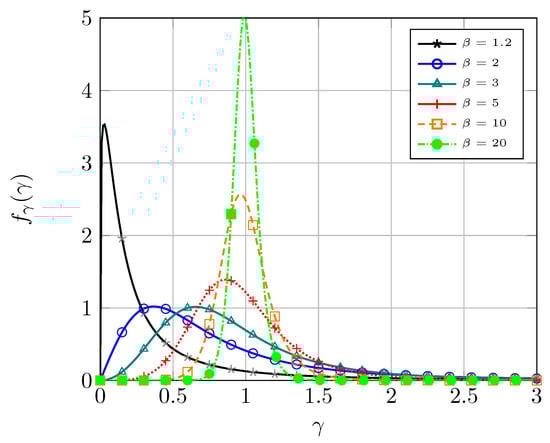
Figure 1.
Probability density function of the received SNR under -distributed fading for different values of . Parameter and then .
Figure 2 shows the AoF as a function of the parameter . We recall that the k-th-order moment of the -distribution is only defined for , so that the AoF is only defined for . We see that low values of correspond to high values of AoF, which implies a rather large fading severity. We see that for , which is coincident with the AoF under Rayleigh fading. Hence, fading severity under -distributed fading can be tuned with parameter , and even exhibiting hyper-Rayleigh behavior [27] in the AoF sense.
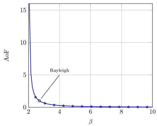
Figure 2.
Amount of fading under -distributed fading for different values of . The case of Rayleigh fading is included as a reference. Solid lines correspond to the theoretical AoF expression in (7). Markers denote MC simulations.
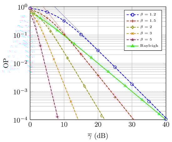
The OP under -distributed fading is evaluated in Figure 3, again when considering different values of the parameter . The SNR threshold value is set to (i.e., dB). We see that the OP dramatically improves for larger values of , which is coherent with the insights obtained by the asymptotic analysis. Specifically, we see that the high-SNR approximation for the OP becomes very tight, and the OP curves have different slope, which only depends on . Interestingly, since the parameter that controls the decay of the OP is enforced to be strictly larger than one due to physical reasons, it is not possible for the -distribution to model an OP decay faster than the Rayleigh case (which always decays with unitary slope). Hence, according to the definition introduced in [27], the -distribution does not exhibit hyper-Rayleigh behavior in the OP sense.
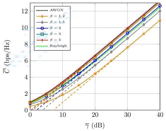
Finally, the average capacity is evaluated in Figure 4, for different values of and including the case of no fading (i.e., AWGN channel) and Rayleigh fading for reference purposes. We see how capacity is decreased when is reduced, which confirms the intuition provided by the asymptotic capacity analysis. We see that low values of can even yield a lower capacity than in the case of Rayleigh fading. Hence, the -distribution is also capable of showing a hyper-Rayleigh behavior in the capacity sense [27]. Conversely, as grows, the capacity gap with respect to the AWGN case (which sets an upper bound because of Jensen’s inequality) is notably reduced.
5. Channel Fitting
In this section, we discuss the implications of the re-parameterization of the LL distribution here proposed when used for channel fitting purposes, identifying some possible issues related to the physical underpinnings of a wireless channel.
With all the previous considerations, the -distribution can be formally used for channel fitting purposes in a physically meaningful way, since establishing a finite value for its parameters and is linked to considering a finite value for the received signal power. Now, this detail has not always been considered in the literature when using the conventional LL distribution for fitting purposes through the parameters and .
For instance, let us first consider the case in [13], on which the use of the LL distribution was proposed to model the misaligned gain in mm-wave systems using an isotropic element pattern. The key motivation for using this distribution lies in its ability to model a heavy-tailed behavior that cannot be reproduced when using the exponential distribution. Now, taking a deep look into the fitting results in [13] (Table III), we see that for all possible combinations of numbers of transmit and receive antennas (i.e., 4, 16, 64, and 256), the best fit was obtained for values of (specifically, ). While this is precisely the case in which the LL distribution has a heavier tail, it also implies that its first-order moment (i.e., the average misaligned gain) is not defined. It is indeed possible to obtain a fitting to empirical data that yields a value of as in [13], e.g., by using some fitting criterion that minimizes some error measure with respect to the empirical distribution. However, it would lack physical meaning when it corresponds to a magnitude for which its statistical average exists (in this case, the average mismatched gain). Thus, caution must be exercised when using these parameter values for performance analysis purposes, since this can affect the definition of the average SNR.
Let us now move to the scenario analyzed in [15], where the LL distribution was used to model fast fading in UAV air-to-ground channels at 1 and 4 GHz, providing better fit results than Rayleigh and Rician distributions. The classical parameterization of the LL distribution through and was used in the fitting. In all instances, values of close to unity were obtained; this is in coherence with the fact that the sample envelopes show a median value close to one, and the parameter is precisely the median of the LL distribution [10]. Now, the fitting results for the amplitude envelope yielded the following values of : {1.41/1.12} and {1.74/1.38} at 1/4 GHz, respectively. However, these values do not seem consistent with the conditions previously defined for the validity of the LL distribution:
- First, for values of , the second-order moment of the LL distribution does not exist. Hence, we have that for the considered set of used in the fitting. This inconsistency can also be seen as follows: if the amplitude envelope , then the power envelope , with and [10]. Hence, we need the condition to be enforced, so that is required when fitting amplitude envelopes.
- Second, in the scenario under consideration, one would anticipate that LOS scenarios exhibit a lower fading severity than the NLOS ones, and that higher frequencies also experience milder fading because of the reduced relative importance of the diffuse components compared to the LOS ones. This is in coherence with the values shown in Figure 5 and Figure 6, on which the fitting (the channel fitting was performed using the cftool included in Matlab, with the criterion of finding the set of parameters () that minimize the root mean square error (RMSE) with respect to the empirical CDF. The empirical CDFs in [15] were obtained by using the tool WebPlotDigitizer, which allows to reverse engineer images of data visualizations to extract the underlying numerical data) over the empirical CDFs given in [16] is carried out using the parameterized version of the LL distribution. We see that the actual values for the parameters should be {6.677/19.9} and {4.244/9.311} for the 1/4 GHz scenarios, respectively. Hence, we confirm that a larger is associated with a milder fading scenario. As stated in [15], the estimated values for the parameter are close to unity in all instances.
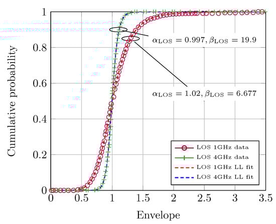
Figure 5.
Statistical distributions of fast fading in UAV air-to-ground channels at 1 and 4 GHz, LOS scenario. Empirical CDF values were obtained from [15], whereas corrected fitting values for the LL distribution are provided here. Goodness-of-fit values are and .
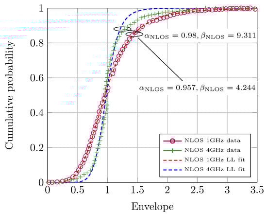
Figure 6.
Statistical distributions of fast fading in UAV air-to-ground channels at 1 and 4 GHz, NLOS scenario. Empirical CDF values were obtained from [15], whereas corrected fitting values for the LL distribution are provided here. Goodness-of-fit values are and .
Our guess is that at some point in the fitting process conducted in [15], there was a mismatch between the parameter of the LL distribution used by the fitting tool, and that corresponded to the LL pdf in ([15], Equation (5)), e.g., maybe using a different parameterization.
6. Conclusions
We introduced the -distribution, a reformulation of the LL distribution that is suited for fading channel modeling purposes. The simple form of its chief statistics facilitates subsequent performance analyses over -distributed fading channels, an aspect which was not previously addressed in the literature so far. Relevant practical issues associated with the use of the LL distribution for channel fitting purposes were discussed.The key role of the shape parameter in capturing fading severity was highlighted, showing that the -distribution can recreate propagation conditions less/more severe than Rayleigh fading, being categorized into the strong hyper-Rayleigh behavior [27].
Author Contributions
Conceptualization, F.J.L.-M.; simulation, I.S.; validation, I.S.; formal analysis, I.S. and F.J.L.-M.; writing, I.S. and F.J.L.-M.; supervision, F.J.L.-M.; funding acquisition, F.J.L.-M. All authors have read and agreed to the published version of the manuscript.
Funding
This work was funded by European Social and Regional Funds and Junta de Andalucía (P18-RT-3175, UMA20-FEDERJA-002), by Universidad de Málaga, and by Universidad de Granada.
Data Availability Statement
Data generated for the elaboration of all figures in the manuscript will kindly be provided by the authors upon reasonable request.
Conflicts of Interest
The authors declare no conflict of interest. The authors gratefully acknowledge the assistance of Gonzalo Javier Anaya-López in the channel fitting procedures described in Section 5.
Abbreviations
The following abbreviations are used in this manuscript:
| AoF | Amount of Fading |
| AWGN | Additive White Gaussian Noise |
| CDF | Cumulative Distribution Function |
| CLT | Central Limit Theorem |
| LL | Log-Logistic |
| LOS | Line-of-Sight |
| MC | Monte Carlo |
| NLOS | Non Line-of-Sight |
| OP | Outage Probability |
| Probability Density Function | |
| RMSE | Root Mean Square Error |
| SNR | Signal to Noise Ratio |
| UAV | Unmanned Aerial Vehicle |
References
- Nakagami, M. The m-Distribution—A General Formula of Intensity Distribution of Rapid Fading. In Statistical Methods in Radio Wave Propagation; Hoffman, W., Ed.; Pergamon Press: Oxford, UK, 1960; pp. 3–36. [Google Scholar] [CrossRef]
- Beckmann, P. Statistical distribution of the amplitude and phase of a multiply scattered field. Res. Natl. Bur. Stand. Radio Propag. 1962, 66D, 231–240. [Google Scholar] [CrossRef]
- Yacoub, M.D. The κ-μ distribution and the η-μ distribution. IEEE Antennas Propag. Mag. 2007, 49, 68–81. [Google Scholar] [CrossRef]
- Yacoub, M.D. The α-μ Distribution: A Physical Fading Model for the Stacy Distribution. IEEE Trans. Veh. Technol. 2007, 56, 27–34. [Google Scholar] [CrossRef]
- Paris, J.F. Statistical Characterization of κ-μ Shadowed Fading. IEEE Trans. Veh. Technol. 2014, 63, 518–526. [Google Scholar] [CrossRef] [Green Version]
- Yoo, S.K.; Cotton, S.L.; Sofotasios, P.C.; Matthaiou, M.; Valkama, M.; Karagiannidis, G.K. The Fisher-Snedecor F Distribution: A Simple and Accurate Composite Fading Model. IEEE Commun. Lett. 2017, 21, 1661–1664. [Google Scholar] [CrossRef] [Green Version]
- Hashemi, H. The indoor radio propagation channel. Proc. IEEE 1993, 81, 943–968. [Google Scholar] [CrossRef]
- Babich, F.; Lombardi, G. Statistical analysis and characterization of the indoor propagation channel. IEEE Trans. Commun. 2000, 48, 455–464. [Google Scholar] [CrossRef]
- Fisk, P.R. The Graduation of Income Distributions. Econometrica 1961, 29, 171–185. [Google Scholar] [CrossRef]
- Muse, A.H.; Mwalili, S.M.; Ngesa, O. On the log-logistic distribution and its generalizations: A survey. Int. J. Stat. Probab. 2021, 10, 93. [Google Scholar] [CrossRef]
- Chamaani, S.; Nechayev, Y.I.; Hall, P.S.; Constantinou, C.; Mirtaheri, S.A. Short-term and long-term fading of in-body to out-of-body channel in MICS band. In Proceedings of the 5th European Conference on Antennas and Propagation (EUCAP), Rome, Italy, 11–15 April 2011; pp. 3797–3800. [Google Scholar]
- Song, D.; Wang, L.; Xu, Z.; Chen, G. Joint Code Rate Compatible Design of DP-LDPC Code Pairs for Joint Source Channel Coding over Implant-to-External Channel. IEEE Trans. Wirel. Commun. 2022. [Google Scholar] [CrossRef]
- Rebato, M.; Park, J.; Popovski, P.; De Carvalho, E.; Zorzi, M. Stochastic Geometric Coverage Analysis in mmWave Cellular Networks With Realistic Channel and Antenna Radiation Models. IEEE Trans. Commun. 2019, 67, 3736–3752. [Google Scholar] [CrossRef] [Green Version]
- Liang, J.; Liang, Q. Outdoor Propagation Channel Modeling in Foliage Environment. IEEE Trans. Veh. Technol. 2010, 59, 2243–2252. [Google Scholar] [CrossRef]
- Cui, Z.; Briso-Rodríguez, C.; Guan, K.; Calvo-Ramírez, C.; Ai, B.; Zhong, Z. Measurement-Based Modeling and Analysis of UAV Air-Ground Channels at 1 and 4 GHz. IEEE Antennas Wirel. Propag. Lett. 2019, 18, 1804–1808. [Google Scholar] [CrossRef]
- Cui, Z.; Briso-Rodríguez, C.; Guan, K.; Zhong, Z.; Quitin, F. Multi-Frequency Air-to-Ground Channel Measurements and Analysis for UAV Communication Systems. IEEE Access 2020, 8, 110565–110574. [Google Scholar] [CrossRef]
- Jiang, W.; Liu, W.; Xu, Z. Experimental Investigation of Turbulence Channel Characteristics for Underwater Optical Wireless Communications. In Proceedings of the 2021 IEEE/CIC International Conference on Communications in China (ICCC), Xiamen, China, 28–30 July 2021; pp. 858–863. [Google Scholar] [CrossRef]
- Kumpuniemi, T.; Hämäläinen, M.; Yazdandoost, K.Y.; Iinatti, J. Human Body Shadowing Effect on Dynamic UWB On-Body Radio Channels. IEEE Antennas Wirel. Propag. Lett. 2017, 16, 1871–1874. [Google Scholar] [CrossRef] [Green Version]
- Rezki, Z.; Alouini, M. On the Capacity of Multiple Access and Broadcast Fading Channels with Full Channel State Information at Low SNR. IEEE Trans. Wirel. Commun. 2014, 13, 464–475. [Google Scholar] [CrossRef] [Green Version]
- Smith, D.B.; Miniutti, D.; Lamahewa, T.A.; Hanlen, L.W. Propagation Models for Body-Area Networks: A Survey and New Outlook. IEEE Antennas Propag. Mag. 2013, 55, 97–117. [Google Scholar] [CrossRef]
- Pittolo, A.; Tonello, A.M. Physical layer security in PLC networks: Achievable secrecy rate and channel effects. In Proceedings of the 2013 IEEE 17th International Symposium on Power Line Communications and Its Applications, Johannesburg, South Africa, 24–27 March 2013; pp. 273–278. [Google Scholar] [CrossRef]
- Ramírez-Espinosa, P.; López-Martínez, F.J. Composite Fading Models Based on Inverse Gamma Shadowing: Theory and Validation. IEEE Trans. Wirel. Commun. 2021, 20, 5034–5045. [Google Scholar] [CrossRef]
- Simon, M.K.; Alouini, M.S. Digital Communication over Fading Channels; John Wiley & Sons: Hoboken, NJ, USA, 2005; Volume 95. [Google Scholar]
- Wang, Z.; Giannakis, G. A Simple and General Parameterization Quantifying Performance in Fading Channels. IEEE Trans. Commun. 2003, 51, 1389–1398. [Google Scholar] [CrossRef] [Green Version]
- Goldsmith, A.J.; Varaiya, P.P. Capacity of fading channels with channel side information. IEEE Trans. Inf. Theory 1997, 43, 1986–1992. [Google Scholar] [CrossRef] [Green Version]
- Yilmaz, F.; Alouini, M.S. Novel asymptotic results on the high-order statistics of the channel capacity over generalized fading channels. In Proceedings of the 2012 IEEE 13th International Workshop on Signal Processing Advances in Wireless Communications (SPAWC), Cesme, Turkey, 17–20 June 2012; pp. 389–393. [Google Scholar] [CrossRef]
- Garcia-Corrales, C.; Fernandez-Plazaola, U.; Cañete, F.J.; Paris, J.F.; Lopez-Martinez, F.J. Unveiling the Hyper-Rayleigh Regime of the Fluctuating Two-Ray Fading Model. IEEE Access 2019, 7, 75367–75377. [Google Scholar] [CrossRef]
Publisher’s Note: MDPI stays neutral with regard to jurisdictional claims in published maps and institutional affiliations. |
© 2022 by the authors. Licensee MDPI, Basel, Switzerland. This article is an open access article distributed under the terms and conditions of the Creative Commons Attribution (CC BY) license (https://creativecommons.org/licenses/by/4.0/).